Modeling Impact of Climate Change on Surface Water Availability Using SWAT Model in a Semi-Arid Basin: Case of El Kalb River, Lebanon

Abstract

Assessing the impact of climate change on streamflow is crucial for depicting the vulnerability of water resources and for identifying proper adaptation measures. This study used the Soil and Water Assessment Tool (SWAT) to simulate the impact of climate change on the streamflow of El Kalb river, a major perennial river in Lebanon. The model performance was tested for monthly flow at two stations under a nine-year calibration period (2003–2011) and a four-year validation period (2012–2015). The model results indicated satisfactory precision in fitting observed and simulated flow using various acceptable statistical indices. Future projections of climate change were obtained for three Representative Concentration Pathways (RCPs) (2.6, 4.5, and 8.5). The model indicated that the average annual discharge of El Kalb River in the near future (2021–2040) will decrease by around 28–29% under the three RCP scenarios. End-of-century projections (2081–2100) indicated that the flow will decrease by 23%, 28%, and 45% under RCP 2.6, RCP 4.5, and RCP 8.5, respectively.

1. Introduction

Long-term records showing the impacts of climate change continue to prove the dire need for sustainable management and planning of water resources. The variation in precipitation due to climate change has had significant repercussions on the supply of water resources [1]. According to the 5th assessment report (AR5) of the Intergovernmental Panel on Climate Change (IPCC), the three-decade period lasting from 1983 to 2012 was likely the warmest 30-year period of the last 1400 years in the northern hemisphere. A linearly rising trend of global warming in the range of 0.65 °C to 1.06 °C over the 1880–2012 period was reported [2]. The United Nation’s 2030 Agenda stipulated one of the indicators for Sustainable Development Goal no. 13 (SDG 13: Climate Action) to specifically assess the number of countries with national adaptation strategies that help consider climate risks when making decisions. This is in coordination with SDG 6 that seeks the sustainable management of water and sanitation systems [3]. Indeed, climate change was found to be the most influential planetary boundary affecting freshwater use [4].

Conceptual and physically based models to assess the impact of climate change on water resources have been used [5]. The Soil and Water Assessment Tool (SWAT), a physically based model, has been used for streamflow prediction [6,7,8,9,10,11]. SWAT is used to address watershed management questions by predicting the effects of changes in soil, land use, and climate on water quantity and quality [12]. Recently, Haghighi et al. [13] used the SWAT model on the Marboreh watershed in Iran to prove that the climate change impact on the hydrology of the watershed is more significant than land-use change. Mittal et al. [14] used the SWAT model on the Kangsabati river in India to show that the combined impact of dam construction and climate change will significantly reduce river flow, while climate change alone will reduce the high peak flows in the near future (2021–2050). Physically based models are used to help assess current and future problems, which is a prerequisite to planning water management policies and strategies [15,16].

Located in the Middle East, Lebanon is considered to have sufficient natural water resources. Yet, its potential annual renewable water resources have decreased from a value of 1155 to 1074 m³/capita/year, between 2002 and 2008 [17]. Access to safe drinking water reaches 37% of the Lebanese population, whereas access to sanitation services reaches only 20% of the population [18]. Most of the water-related challenges in Lebanon have been attributed to poor management and planning and outdated legislations [19,20]. The country’s score in the degree of implementation of integrated water resources management is medium to low, implying that implementation is taking place but with limited geographic coverage and stakeholder participation [21]. The decrease in snowpack melt rate changed from 97 days prior to 2000 to 86 days during the period of 2000–2010, and to 64 days during the period of 2010–2018 [22]. Furthermore, defining the exact number of rivers in Lebanon has become a source of debate as some rivers remain dry for more than 9 months a year and 60% of springs have disappeared [22]. Discharge from rivers such as Litani river, Al Kabir river, and El Damour river decreased on average by 40%, while that of Beirut river decreased by 55% [22]. The flow of 12 perennial rivers in Lebanon decreased by 23% in 40 years, compared to the year 1965 [23]. Similarly, the flow of 60 seasonal watercourses decreased by 50% below normal levels [24]. In addition, the Litani river, the largest river in length and width in Lebanon, showed a drying trend in the period between 1900 and 2008, with a reduction rate varying between 0.1 and 0.8 m³/s per decade [25]. The cost of reduced agricultural, domestic, and industrial water supply due to climate change was estimated at USD 21 million, USD 320 million, and USD 1200 million by 2020, 2040, and 2080, respectively. Similarly, the reduction in water supply for the generation of hydroelectricity was estimated at USD 3 million, USD 31 million, and USD 110 million by 2020, 2040, and 2080, respectively [26].

At the level of water demand, a 10% climate-induced increase in total water demand is anticipated in Lebanon by 2050 [27]. The COVID-19 pandemic is further expected to exacerbate current conditions where water demand is estimated to have increased by 9 to 12 L per person per day for need of better sanitation [28]. The country is already using more than two-thirds of its available water resources with an anticipated 22% increase in total annual demand by 2035 [29]. Considering the current deficiency in the national water budget, and the low national water storage capacity (6% compared to 85% MENA average), the country is highly susceptible to water shortage [30]. The water deficit is expected to reach 610 million cubic meters by 2035 [31].

According to the third national communication to the United Nations Framework Convention on Climate Change by the Ministry of Environment, viable adaptation measures in the water sector include: establishing reliable data collection and storage systems, improving the feasibility of alternative sources of water, and developing climate-based watershed management plans [26]. Yet, informed decision-making and planning require reliable projections of water quantities. Despite the reported attempts to forecast the impact of climate change on the water sector in Lebanon, river management requires more extensive research in terms of physically based hydrological modeling; only seven studies have addressed the impact of climate change on water quantity and four have modeled the impact of climate change on streamflow [15]. This research assessed the impact of climate change on the streamflow of the El Kalb river, a major perennial river in Lebanon. A physically based model, SWAT, and three climatic scenarios (RCP 2.6, RCP 4.5, and RCP 8.5) were used to simulate the watershed hydrology and to forecast the potential short- and long-term flow changes. This research will contribute to the evaluation and planning objectives under future climate conditions, especially for the projected planned treatment plants along the river stretch.

2. Materials and Methods

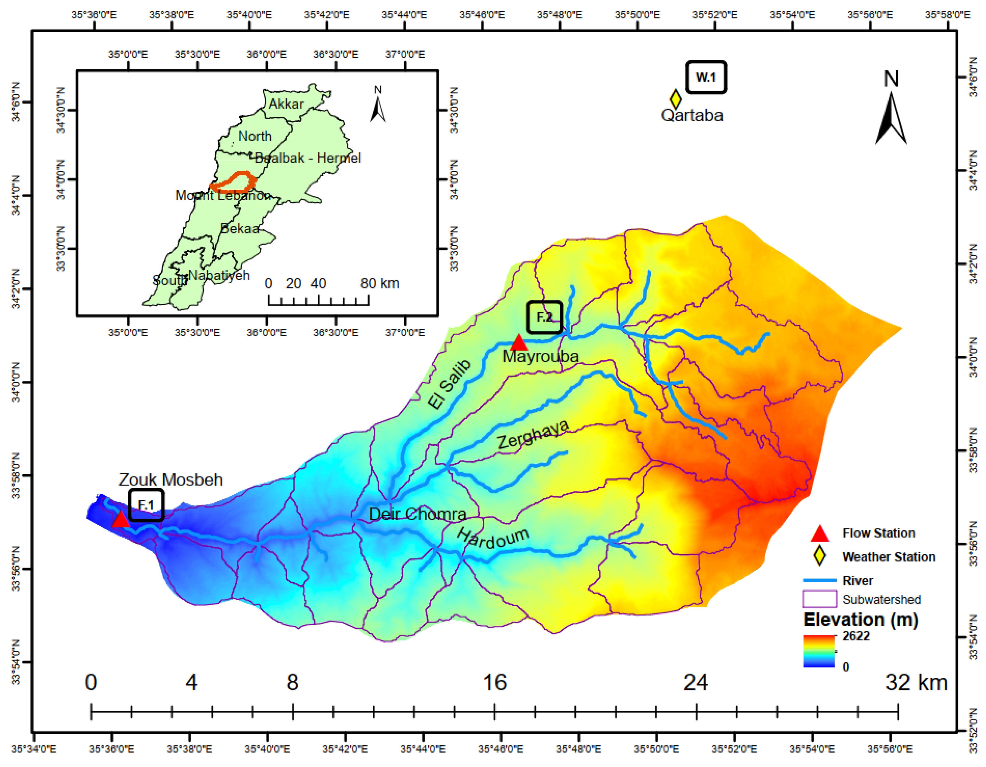
The studied watershed includes a major historical river in Lebanon, El Kalb River, located in the country’s west central administrative governate, Mount Lebanon (Figure 1). The watershed has an area of 252 km², covering an altitude ranging from 0 m near its estuary (at sea mouth to the east) to 2622 m at the hilltops of Sannine to the west where it originates with an average annual precipitation of 1093 mm. The three main tributaries—Zerghaya, El Salib, and Hardoum—join at their confluence in Deir Chomra to form the El Kalb river that discharges in the Mediterranean Sea with an average river discharge of 5.6 m³/s [32].

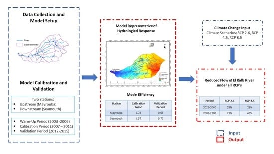
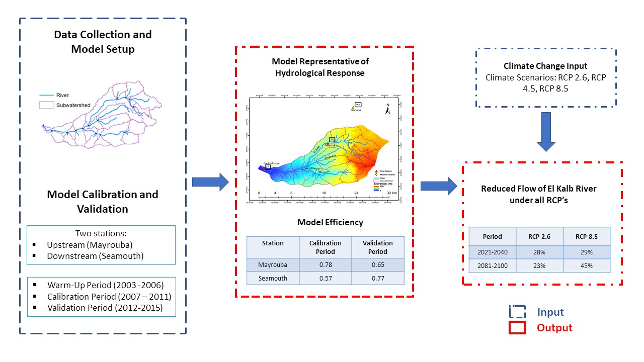
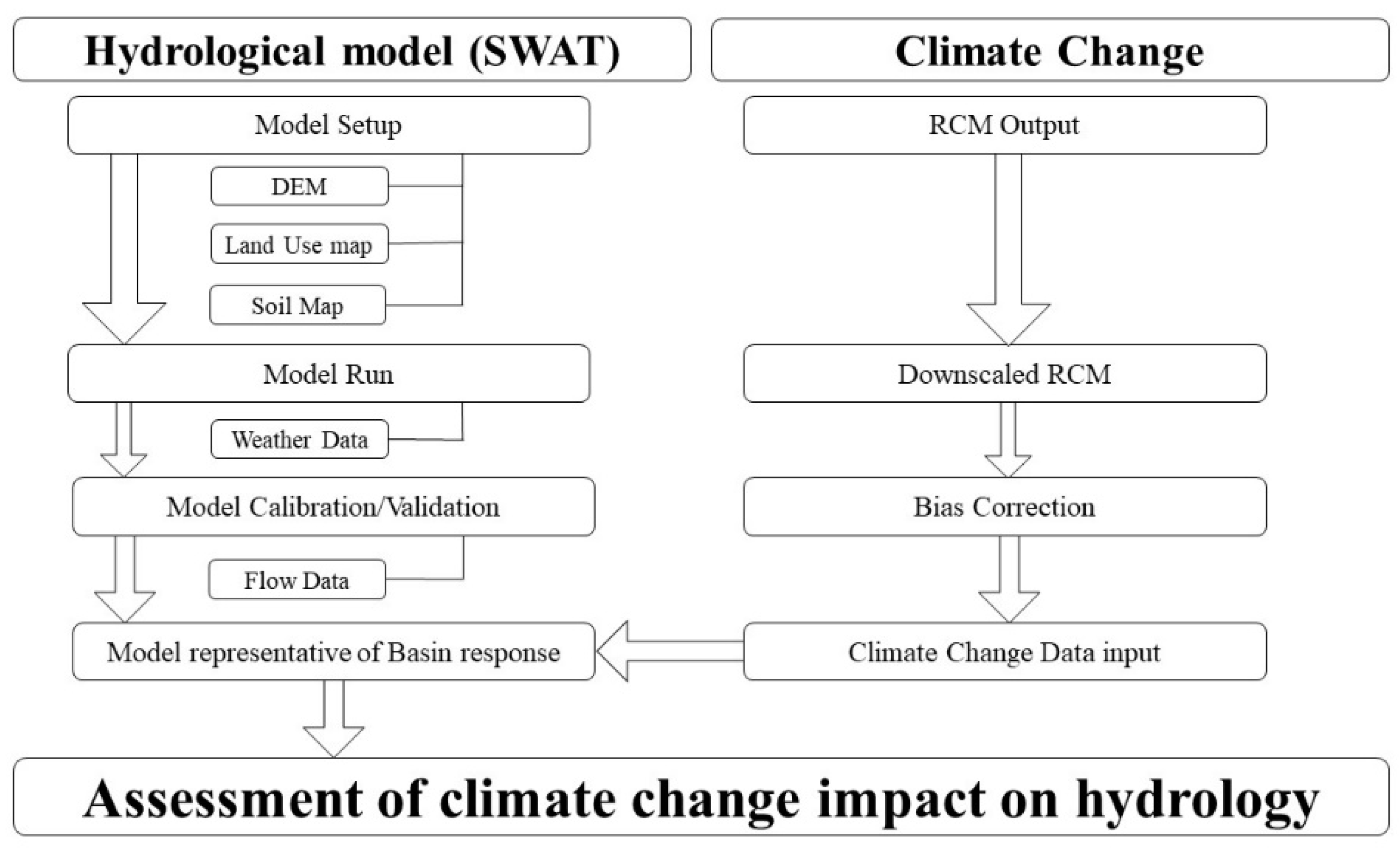
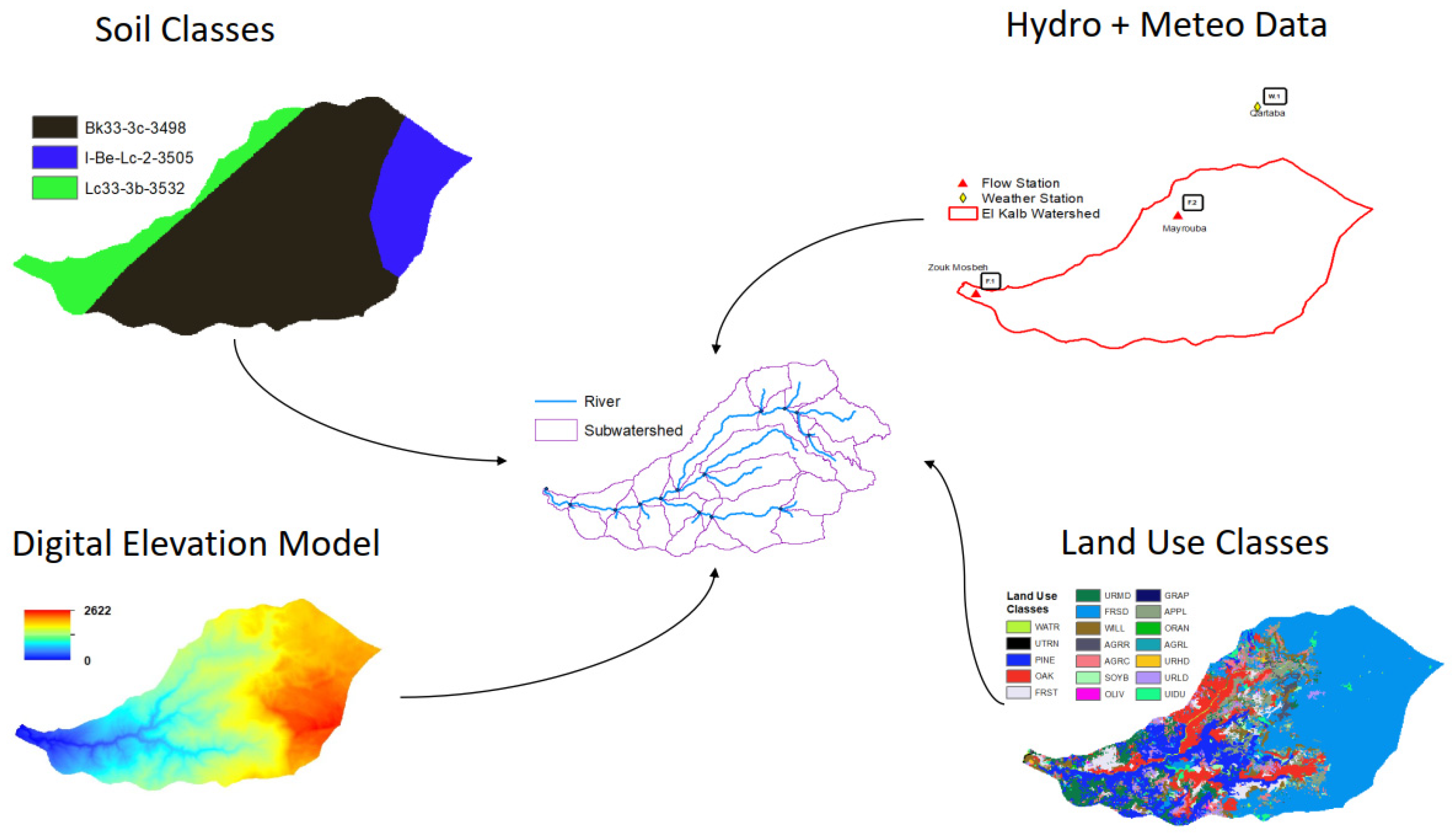
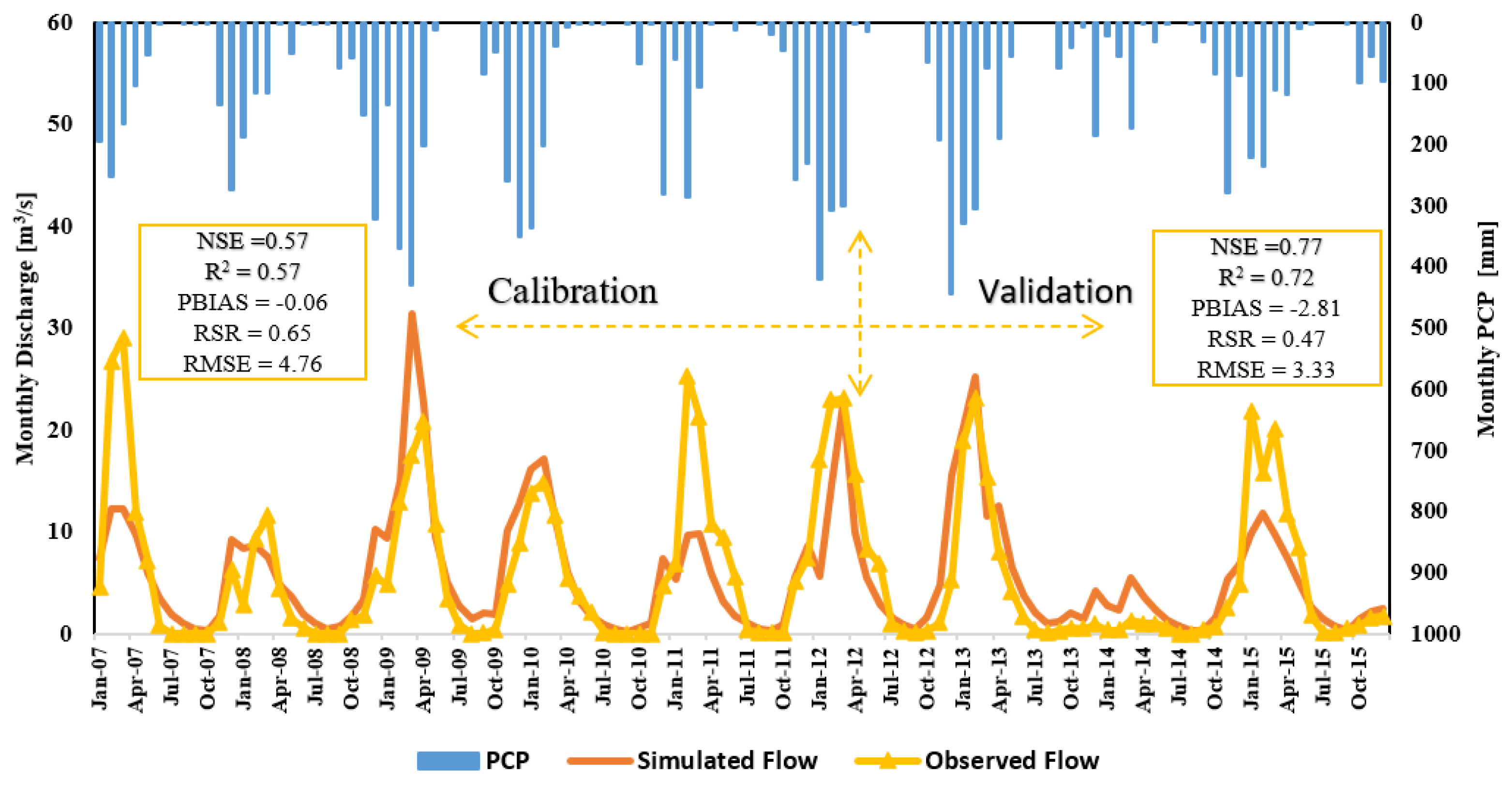
Figure 2 illustrates the methodology used in this study. Three input datasets, describing the physical features of the basin, were used: Digital Elevation Model (DEM), land-use map, and soil map. The basin’s response was simulated at the level of multiple Hydrologic Response Units (HRUs). Historical climatic data were used to calibrate the model for the years 2003 to 2011, after which the model was validated for 4 years (2012 to 2015). Climate change data, retrieved from a Regional Climate Model (RCM), were downscaled and bias-corrected, and then used to model the impact of projected climatic change on the river flow.

The Soil and Water Assessment Tool (SWAT), a physically based hydrological model, was adopted to simulate flow in the watershed. Developed by the United States Department of Agriculture (USDA), SWAT is a deterministic semi-distributed model that divides the catchment into HRUs based on a unique set of data, including land use/cover, soil type, and slope. SWAT models the land phase of the hydrologic cycle using the water balance equation (Equation (1)) [33]:

$$S{W}_t=S{W}_o+{\displaystyle \sum }_{i=1}^t\left(R_{day}-Q_{surf}-E_a-w_{seep}-Q_{gw}\right)$$

(1)

where SW_t is the final soil water content (mm), SW₀ is the initial soil water content on day i (mm), t is the time (days), R_day is the amount of precipitation on day i (mm), Q_surf is the amount of surface runoff on day i (mm), E_a is the amount of evapotranspiration on day i (mm), w_seep is the amount of water entering the vadose zone (unsaturated zone; saturated zone) from the 0 soil profile on day i (mm), and Q_gw is the amount of return flow on day i (mm).

The model requires a specific set of input data, including topography, land use/land cover, soil, and weather data (

Table 1. Spatial model input for El Kalb the Kalb study site.

Data Type	Description/Scale	Source
Topography	DEM Resolution: 10 m	CNRS-2010
Land Use/Land Cover	Cell size: 10 m × 10 m	CNRS-2010
Soil	The Global Soil Map 1: 5,000,000	FAO-DSMW
Weather Data (Historical)	2003–2015 (Daily)	LRA
Flow Data (Historical)	2003–2015 (Monthly)	LRA

and

Table 2. Soil characteristics for El Kalb the Kalb study site.

Parameter	Soil Texture
	Clay Loam	Loam	Clay
Moist Bulk Density (g/cm3)	1.2	1.4	1.4
Depth from soil surface to bottom of soil layer (mm)	300	300	300
Available water capacity (mm H2O/mm soil)	0.37	0.37	0.37
Saturated hydraulic conductivity (mm/hr)	12.43	6.93	4.55
Clay content (% of soil weight)	36	24	40
Silt content (% of soil weight)	39	28	31
Sand content (% of soil weight)	25	48	29
Max rooting depth of soil (mm)	570	690	740

, Figure 3). The basin was divided into 27 subbasins and 123 HRUs. Data were retrieved from the National Council for Scientific Research (CNRS), Food and Agriculture Organization Digital Soil Map of the World (FAO-DSMW), and the Litani River Authority (LRA). DEM, soil, land use, flow, and weather data were used for the model run, model calibration, and validation.

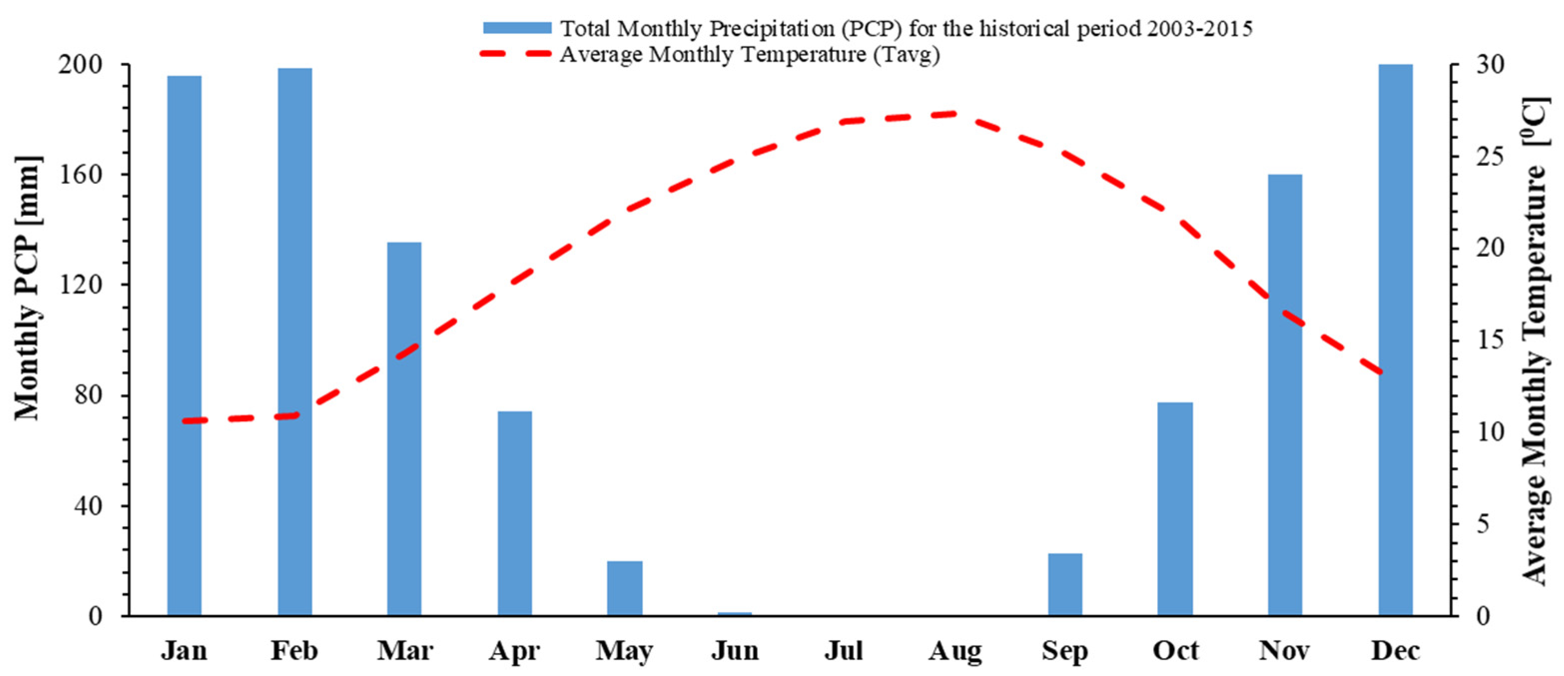
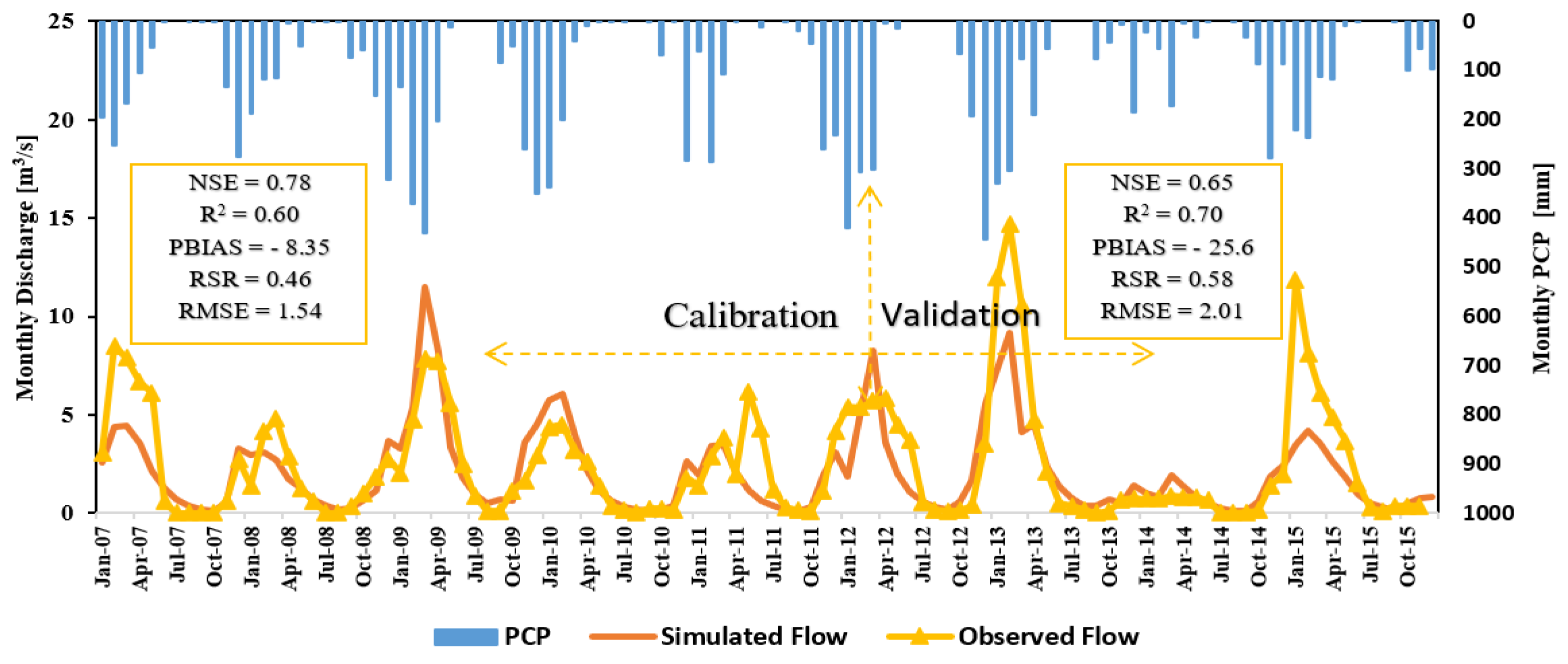
The past flow and weather data (from 2003 till 2015) were used for: model warm-up (2003–2006), calibration (2007–2011), and validation (2012–2015). The data were retrieved from the records of two flow stations (in Zouk Mosbeh city and Mayrouba village) and one weather station (in Qartaba village) (

Table 3. Characteristics of stations.

Station Type	Station Name	Location	Latitude	Longitude	Elevation (m)
Flow	F.1	Seamouth	35:57:02	35:36:22	12
Flow	F.2	Mayrouba	34:00:35	35:46:44	1178
Weather	W.1	Qartaba	34:05:44	35:50:55	1222

). As the weather station inside the watershed had only six years of data, Qartaba weather station, 5 km outside the watershed, was used. Air temperature and precipitation data for both stations were compared using overlapping years that showed similar seasonal patterns. Weather data include daily precipitation (mm), daily maximum and minimum temperature (°C), solar radiation (W/m²), wind speed (m/s), and relative humidity (%). Monthly precipitation and temperature over the past period are shown in Figure 4, where the average yearly precipitation is 1093 mm with an average of 82 wet days, and the average temperature is 15.88 °C.

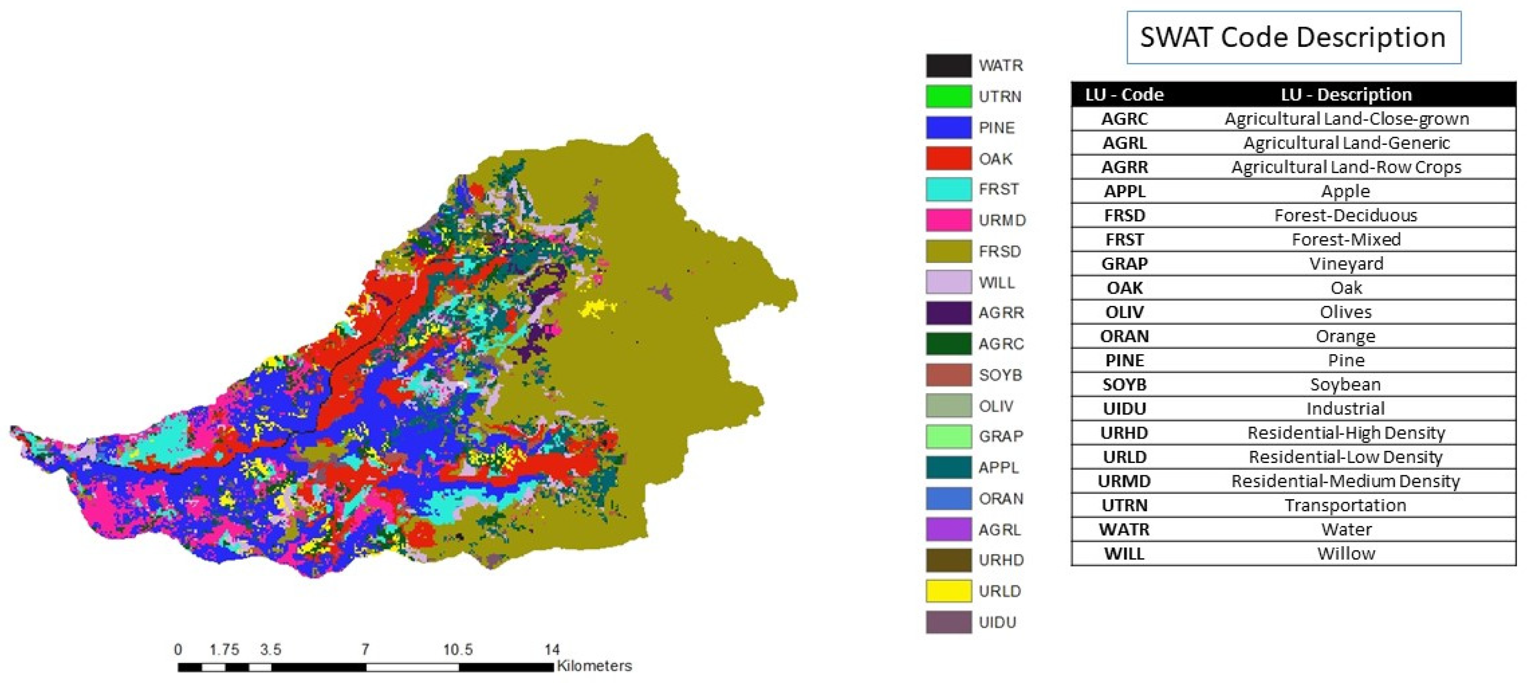
The study area includes 19 land use/land cover classes dominated by deciduous forest (42.58%). Only 9.45% of the land use is urban, of which 63% is residential of medium density (Figure 5). Most rural land cover is covered by wild trees such as oak and pine, as well as apple and other fruit trees. The soil map was obtained from Digital Soil Map of the World [34], and three main soil types are found in the watershed (clay, clay loam, and loam), with clay as the dominant soil.

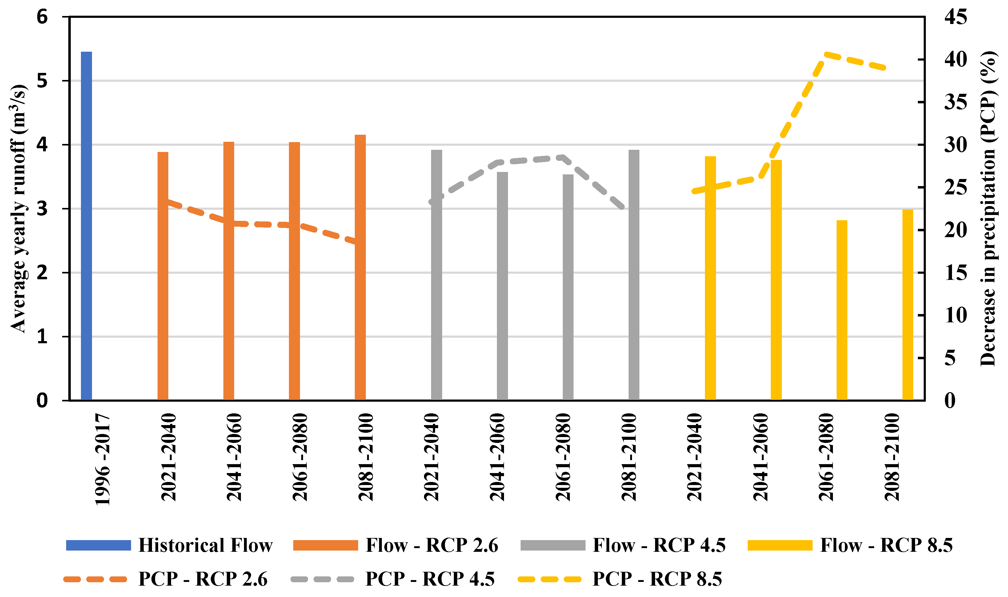
To quantify the impact of climate change on the streamflow of EL Kalb river, projected weather parameters were used for different climate scenarios. Those were adopted from the output of the Coordinated Regional Downscaling Experiment (CORDEX), and obtained from the Lawrence Livermore National Laboratory at the Earth System Grid Federation (ESGF) [35,36]. The scenarios considered in this study cover the Representative Concentration Pathways (RCPs) 2.6, 4.5 and 8.5.

The driving model used was MPI–ESM–MR, which is a General Circulation Model (GCM) developed by the Max Planck Institute for Meteorology Climate Service Center. Due to its relatively coarse scale (grid resolution 0.44°), the GCM was dynamically downscaled using the REMO 2009 regional climate model (RCM). Due to the geographical difference (0.147°) between the station in Qartaba and the center of the nearest grid cell, bias correction was needed during the calibration stage. The downloaded simulated climate change data cover future and historical (overlapping observed weather data from Qartaba station) periods. The simulated climate change data for the El Kalb watershed were prepared using the CMhyd (Climate Model data for hydrological modelling) [37]. Bias correction was performed as the spatial resolution of the General Circulation Models (GCMs) is generally too coarse to be directly used in fine-scale impact studies [38,39]. Bias correction was applied on temperature and precipitation using the additive linear scaling and multiplicative linear scaling methods, respectively, on the overlapping historical period [40]. The future weather data, covering the timespan from 2021 to 2100, were divided into four 20-year periods for future predictions (

Table 4. Change in average interannual temperature in °C.

Period	Past Period	RCP 2.6	Increase (°C)	RCP 4.5	Increase (°C)	RCP 8.5	Increase (°C)
2021–2040	15.93	16.27	0.34	16.24	0.31	16.53	0.60
2041–2060	15.93	16.14	0.22	16.87	0.94	17.27	1.34
2061–2080	15.93	16.25	0.33	17.35	1.42	18.68	2.75
2081–2100	15.93	15.87	−0.06	17.15	1.22	20.32	4.39

).

3. Results

3.1. Model Calibration and Validation

During the tested period 2003–2015, average flows were observed to be 6.62 m³/s and 2.68 m³/s at Seamouth and Mayrouba stations, respectively, under an average annual precipitation of 1092.7 mm and 82 wet days. Calibration was carried out using the observed monthly streamflow data at Seamouth (F.1) and Mayrouba (F.2) for the period 2003 to 2011 (with a warm-up period of 4 years). The model was calibrated manually by changing the parameters for runoff, groundwater, evapotranspiration, snowmelt, and soil. Validation was performed over the observed streamflow data for the period 2012–2015.

Parameters describing the diverse hydrological conditions and characteristics across the watershed were calibrated to physically plausible parameter values [41]. Best-fit parameters are presented in

Table 5. Change in average yearly temperature in °C. The periods used were 2021–2040, 2041–2060, 2061–2080, and 2081–2100 under RCP 2.6, RCP 4.5, and RCP 8.5.

Period	Parameter		Range	Initial Value	Best Fit Value
	Name	Description
Basin	ESCO	Soil evaporation compensation factor	0.01–1	0.95	0.99
	EPCO	Plant uptake compensation factor	0–1	1	0.95
	FFCB	Initial soil water storage expressed as a fraction of field capacity water content	1–1	1	0.95
	SURLAG	Surface runoff lag coefficient (days)	1–24	4	1
	TIMP	Snowpack temperature lag factor	0–1	1	0.5
Management	CN2	Initial SCS runoff curve number for moisture condition II	35–98	Varying †	11%
Soil	SOL_AWC	Available water capacity of the soil (mm H2O/mm soil)	0–1	Varying ‡	245%
	SOL_K	Saturated hydraulic conductivity (mm/h)	0–2000	Varying ‡	14%
Groundwater	GW_DELAY	Groundwater Delay (days)	0–500	Varying ‡	−15%
	ALPHA_BF	Baseflow alpha factor (days)	0–1	0.048	0.5
	GW_QMIN	Threshold depth of water in the shallow aquifer required for return flow to occur (mm)	0–5000	1000	500
	REVAP_MIN	Threshold depth of water in the shallow aquifer required for revap to occur (mm)	0–1000	750	850
HRU	LAT_TIME	Lateral flow travel time (in days)	0–180	0	50

^† Initial values vary according to the land use class. ^‡ Initial values vary according to the soil layer class.

that show the most sensitive parameters. Snow is a major contributor to the water balance in El Kalb watershed, and as such, the snow melt base temperature was adjusted to 0.5 °C with a maximum and minimum snow melt rate of 8.5 mm/°C·d and 2.5 mm/°C·d, respectively. This increased the lag time for snow to melt, infiltrate into the ground, and reach the river as baseflow. Using the Soil Conservation Service (SCS) curve number method to estimate surface runoff in the watershed, the curve number (CN) was increased in several sub-watersheds downstream of the river where urbanization is dominant near the river outlet. In addition, the evapotranspiration method that produced the most reasonable values for the watershed was the Hargreaves method [42] as compared to the Penman Monteith method (

Table 6. Comparison of ET methods in calibration period.

ET Method	Calibration Results (Average Historical Yearly Flow Is 6.185 m3/s)—2006 to 2011
	Simulated Annual Flow (m3/s)	R2	PBIAS
Penman–Monteith	2.251	0.2478	−63.603
Hargreaves	6.032	0.354	−2.619

). The Penman–Monteith method overestimated the ET rates and underestimated the flows [33,36,37].

Other calibration parameters adjusted in this study included the surface runoff lag coefficient (SURLAG), and the initial soil water storage expressed as a fraction of field capacity water content (FFCB). Calibration parameters were based on a literature review, and adjustments were made to peak flows and base flows.

The simulated and observed monthly streamflow at the two stations in the two subbasins (11 and 15) are plotted in Figure 6 and Figure 7. The simulations were initially evaluated by examining the plots visually for a match between the observed and predicted values (Figure 7). Performance measures indicate that the model was able to simulate the discharge of the river at different subbasins with satisfactory to good results.

In addition to graphical methods such as hydrographs, the model performance was also evaluated using the statistical indices, including the Nash–Sutcliffe efficiency (NSE) [43], the RMSE-observations standard deviation ratio (RSR), and the percent bias (PBIAS) [44]. The statistical indices and related equations are presented in

Table 7. Statistical indices for SWAT model [45,46].

Statistical Index	Equation	Indication
Nash–Sutcliffe Efficiency (NSE)	$NSE=1-\frac{{{\displaystyle \sum }}_{i=1}^n\left(Q_{obs}^i-Q_{sim}^i\right)}{{{\displaystyle \sum }}_{i=1}^n\left(Q_{obs}^i-Q_{obs}^{mean}\right)}$	Indicates how well fitted a plot of a 1:1 line of observed vs. simulated data would be.
Standard Deviation Ratio (RSR)	$RSR=\frac{\sqrt{{{\displaystyle \sum }}_{i=1}^n{(Q_{obs}^i-Q_{sim}^i)}^2 }}{\sqrt{{{\displaystyle \sum }}_{i=1}^n{(Q_{obs}^i-Q_{obs}^{mean})}^2}}$	Incorporates the benefits of error index statistics and indicates the standardized error.
Percent Bias (PBIAS)	$PBIAS=\frac{{{\displaystyle \sum }}_{i=1}^n\left(Q_{obs}^i-Q_{sim}^i\right)}{{{\displaystyle \sum }}_{i=1}^n\left(Q_{obs}^i\right)}\times 100$	Measures the average tendency of the simulated data to be larger or smaller than their observed counterparts.

Where $Q_{obs}^i$ and $Q_{sim}^i$ are the observed and simulated streamflow at the i time step, respectively; $Q_{obs}^{mean}$ is the average of the observed streamflow; n is the number of observations.

[45].

The calibration and validation model performance statistics are presented in

Table 8. Monthly flow calibration and validation statistics of the measured and simulated data at F1 and F2 stations.

Statistical Index	Seamouth		Mayrouba
	Calibration	Validation	Calibration	Validation
NSE	0.57	0.77	0.78	0.65
PBIAS	−0.06	−2.81	−8.35	−25.60
RSR	0.65	0.47	0.46	0.58

. According to Moriasi et al. [45], during the calibration period, at Station F1, the model performance was satisfactory (NSE = 0.57 ∑ (0.5; 0.65), PBIAS = 0.06% < ±10%), while at station F2, the model performance was in a very good range (NSE = 0.78 ∑ (0.75; 1), PBIAS = −8.35% < ±10%).

3.2. Impact of Climate Change

As precipitation is the main driver of river flow, the variation in El Kalb river flow at station F.1 (Seamouth) is plotted along with the change in yearly precipitation for the three RCPs (Figure 8). Compared to the average yearly actual runoff of 5.47 m³/s for the past period (1998–2017), the results of introducing the MPI–ESM–MR model data into the SWAT model indicated that, in the near future (2021–2040), the average annual simulated flow will decrease to 3.925, 3.957, and 3.862 m³/s under RCP 2.6, RCP 4.5, and RCP 8.5, respectively (equivalent to decreases of 28%, 28%, and 29%, respectively). End-of-century (2081–2100) simulations indicated a flow reduction to 4.196, 3.960, and 3.017 m³/s under RCP 2.6, RCP 4.5, and RCP 8.5, respectively (equivalent to decreases of 23%, 28%, and 45%, respectively). The greatest reduction in runoff is expected to occur under RCP 8.5. This is compatible with the results of other studies [13,47].

Based on Figure 8, precipitation will decrease with time compared to the recorded past period under all three RCPs. Under RCP 2.6, the maximum amount of precipitation (minimum decrease) is expected to occur by 2081–2100, whereas the minimum amount of precipitation (maximum decrease) is expected to occur by 2061–2080. Average yearly flow is thus minimum during 2061–2080 (when mean annual temperature would have increased by 2.75 °C) with a value of 2.98 m³/s (45.5% decrease in flow from the historical value of 5.47 m³/s). On the other hand, the maximum average yearly flow will occur at the end of the century (2081–2100) under RCP 2.6 with a value of 4.15 m³/s (24.1% decrease). Furthermore, though RCP 8.5 is the extremely pessimistic pathway, its simulated flow during the first two periods (2021–2040 and 2041–2060) is not very different from that of RCP 4.5 (it is even higher).

Table 9. Average monthly observed flows (in m³/s) of El Kalb river during the historical period and average future simulated flows during the periods 2021–2040 and 2041–2061 and under RCP 2.6, RCP 4.5, and RCP 8.5.

	Period	2021–2040			2041–2060
Month *	Historic	RCP 2.6	RCP 4.5	RCP 8.5	RCP 2.6	RCP 4.5	RCP 8.5
January	9.470	8.009	6.842	7.200	7.475	6.008	8.001
February	14.964	11.442	10.886	11.519	10.794	9.566	10.942
March	14.251	7.987	9.112	8.374	8.465	7.543	8.199
April	10.366	5.179	5.710	4.954	5.850	4.862	5.014
May	5.510	3.105	3.457	3.040	3.806	3.072	2.962
June	2.306	1.945	2.149	2.014	2.288	2.251	2.334
July	0.548	1.135	1.218	1.222	1.270	1.246	1.103
August	0.161	0.588	0.632	0.634	0.660	0.647	0.568
September	0.139	0.302	0.326	0.329	0.342	0.335	0.292
October	0.387	0.267	0.344	0.276	0.274	0.345	0.299
November	2.444	3.032	2.516	2.773	3.440	3.266	2.167
December	5.077	4.114	4.296	4.003	4.331	4.139	3.705
Minimum	0.139	0.267	0.326	0.276	0.274	0.335	0.292
Average	5.469	3.925	3.957	3.862	4.083	3.607	3.799
Maximum	14.964	11.442	10.886	11.519	10.794	9.566	10.942

* The monthly flow for each 20-year period is the average flow of each month across the 20 years.

and

Table 10. Average monthly observed flows (in m³/s) of El Kalb river during the historical period and average future simulated flows during the periods 2061–2080 and 2081–2100 and under RCP 2.6, RCP 4.5, and RCP 8.5.

	Period	2061–2080			2081–2100
Month *	Historic	RCP 2.6	RCP 4.5	RCP 8.5	RCP 2.6	RCP 4.5	RCP 8.5
January	9.470	8.199	6.845	5.433	8.532	7.685	5.486
February	14.964	10.993	10.048	8.574	11.594	10.917	8.633
March	14.251	8.725	7.769	6.186	8.357	7.790	6.059
April	10.366	5.311	4.941	3.915	5.651	5.302	3.656
May	5.510	3.177	2.849	2.395	3.457	3.330	2.070
June	2.306	2.446	1.832	1.404	2.335	2.478	1.169
July	0.548	1.478	1.046	0.771	1.294	1.287	0.602
August	0.161	0.772	0.539	0.389	0.675	0.667	0.298
September	0.139	0.403	0.276	0.195	0.351	0.346	0.145
October	0.387	0.455	0.300	0.189	0.445	0.416	0.301
November	2.444	2.573	2.640	1.919	3.219	3.192	3.505
December	5.077	4.341	3.740	2.797	4.444	4.107	4.286
Minimum	0.139	0.403	0.276	0.189	0.351	0.346	0.145
Average	5.469	4.073	3.569	2.847	4.196	3.960	3.017
Maximum	14.964	10.993	10.048	8.574	11.594	10.917	8.633

* The monthly flow for each 20-year period is the average flow of each month across the 20 years.

show the monthly average discharge during the four simulated periods under the three studied RCPs. In all scenarios and all periods, the maximum monthly flow always occurs in February. However, while the minimum flow is mostly observed during the month of September, it shifts to the month of October twice under RCP 2.6 (2021–2040 and 2041–2060) and twice under RCP 8.5 (2021–2040 and 2061–2081), which indicates a possibility of broadening the dry period.

Implications of the expected changes are of high relevance to the future as decisionmakers can now reconsider the driest and wettest months of El Kalb in their water strategies and policies. In addition, the model can be further used for research on watershed-related activities such as the impact of the planned dams on the hydrology of the watershed and the impact of planned wastewater treatment plants on the river’s water quality [48]. Future studies may also address restoring the river flow lost due to climate change from the proposed plant effluent, in addition to modeling the impact of effluent on river water quality. Under proper design, the plant effluent comprising treated wastewater may be used for ornamental and environmental purposes to restore the river flow lost due to climate change [49,50]. In addition, this model can be used to assess the impact of the WWTP effluent on river water quality.

4. Conclusions

The physically based semi-distributed SWAT model was capable of satisfactorily simulating the monthly flow of El Kalb basin in Lebanon. Climate change scenarios were employed for three RCPs and four 20-year periods. Summarizing the results, the main findings of this study are the following:

• The simulated flow will decrease by 28%, 28%, and 29% under RCP 2.6, RCP 4.5, and RCP 8.5, respectively, in the near future (2021–2040). On the other hand, the simulated flow will decrease by 23%, 28%, and 45% under RCP 2.6, RCP 4.5, and RCP 8.5, respectively, during the end of the century (2081–2100).
• The greatest change will occur under RCP 8.5, during 2061–2080. By then, the mean annual temperature is expected to increase by 2.75 °C and the mean annual precipitation is expected to decrease by 40.6%, which will decrease the flow from 5.47 m³/s to 2.98 m³/s (45.5% decrease).
• The maximum monthly flow will remain during the month of February for all three RCPs and during all the four periods. The anticipated climate change RCPs showed that the decrease in rainfall and increase in temperature will be the main factors influencing the reduction in water availability.
• Snow melt was a significant parameter affecting the calibration phase, where the calibration required increasing the maximum snow melt rate to 8.5 mm/°C.d.
• Research findings could contribute to an effective management of El Kalb basin seeing that there are projected planned WWTP along the river stretch. Recommendations for further research include model simulation on a daily time step, simulating the impact of climate change on water quality of El Kalb river, and assessing the effect of the dams on the hydrological cycle in the watershed.

References

1. Busico, G.; Ntona, M.M.; Carvalho, S.C.P.; Patrikaki, O.; Voudouris, K.; Kazakis, N. Simulating Future Groundwater Recharge in Coastal and Inland Catchments. Water Resour. Manag. 2021, 1–16. [Google Scholar] [CrossRef]
2. Change, I.C. Climate Change 2014 Synthesis Report Summary Change; IPCC: Geneva, Switzerland, 2014; ISBN 9789291691432. [Google Scholar]
3. UN Statistical Commission. Global Indicator Framework for the Sustainable Development Goals and Targets of the 2030 Agenda for Sustainable Development; UN Statistical Commission: New York, NY, USA, 2017.
4. Mathias, J.-D.; Anderies, J.M.; Janssen, M. On our rapidly shrinking capacity to comply with the planetary boundaries on climate change. Nature 2017, 7, 1–9. [Google Scholar] [CrossRef] [Green Version]
5. Skoulikaris, C.; Ganoulis, J. Climate change impacts on river catchment hydrology using dynamic downscaling of global climate models. In National Security and Human Health Implications of Climate Change; Fernando, H.J.S., Klaic, Z.B., McCulley, J.L., Eds.; Springer: Dordrecht, The Netherlands, 2011; ISBN 9789400725003. [Google Scholar]
6. Bieger, K.; Hörmann, G.; Fohrer, N. Simulation of streamflow and sediment with the soil and water assessment tool in a data scarce catchment in the three gorges region, china. J. Environ. Qual. 2014, 43, 37–45. [Google Scholar] [CrossRef]
7. Cambien, N.; Gobeyn, S.; Nolivos, I.; Eurie Forio, M.A.; Arias-Hidalgo, M.; Dominguez-Granda, L.; Witing, F.; Volk, M.; Goethals, P.L.M. Using the soil and water assessment tool to simulate the pesticide dynamics in the data scarce guayas River Basin, Ecuador. Water 2020, 12, 696. [Google Scholar] [CrossRef] [Green Version]
8. Duru, U.; Arabi, M.; Wohl, E.E. Modeling stream flow and sediment yield using the SWAT model: A case study of Ankara River basin, Turkey. Phys. Geogr. 2018, 39, 264–289. [Google Scholar] [CrossRef]
9. Golmohammadi, G.; Prasher, S.; Madani, A.; Rudra, R. Evaluating three hydrological distributed watershed models: MIKE-SHE, APEX, SWAT. Hydrology 2014, 1, 20–39. [Google Scholar] [CrossRef] [Green Version]
10. Golmohammadi, G.; Rudra, R.; Dickinson, T.; Goel, P.; Veliz, M. Predicting the temporal variation of flow contributing areas using SWAT. J. Hydrol. 2017, 547, 375–386. [Google Scholar] [CrossRef]
11. Grusson, Y.; Sun, X.; Gascoin, S.; Sauvage, S.; Raghavan, S.; Anctil, F.; Sáchez-Pérez, J.M. Assessing the capability of the SWAT model to simulate snow, snow melt and streamflow dynamics over an alpine watershed. J. Hydrol. 2015, 531, 574–588. [Google Scholar] [CrossRef]
12. Gassman, P.W.; Reyes, M.R.; Green, C.H.; Arnold, J.G. The Soil and Water Assessment Tool: Historical Development, Applications, and Future Research Directions. Trans. ASABE 2007, 50, 1211–1250. [Google Scholar] [CrossRef] [Green Version]
13. Torabi Haghighi, A.; Darabi, H.; Shahedi, K.; Solaimani, K.; Kløve, B. A Scenario-Based Approach for Assessing the Hydrological Impacts of Land Use and Climate Change in the Marboreh Watershed, Iran. Environ. Model. Assess. 2020, 25, 41–57. [Google Scholar] [CrossRef] [Green Version]
14. Mittal, N.; Bhave, A.G.; Mishra, A.; Singh, R. Impact of human intervention and climate change on natural flow regime. Water Resour. Manag. 2016, 30, 685–699. [Google Scholar] [CrossRef] [Green Version]
15. Saade, J.; Atieh, M.; Ghanimeh, S. Overview of Hydrological Modeling of Climate Impacts on Rivers in the Mediterranean and Lebanon. In Proceedings of the 2019 Fourth International Conference on Advances in Computational Tools for Engineering Applications (ACTEA), Beirut, Lebanon, 3–5 July 2019; pp. 1–6. [Google Scholar] [CrossRef]
16. Hanson, R.T.; Flint, L.E.; Flint, A.L.; Dettinger, M.D.; Faunt, C.C.; Cayan, D.; Schmid, W. A method for physically based model analysis of conjunctive use in response to potential climate changes. Water Resour. Res. 2012, 48, 1–23. [Google Scholar] [CrossRef]
17. United Nations Development Programme. Water Governance in the Arab Region: Managing Scarcity and Securing the Future; United Nations Publications: New York, NY, USA, 2013; ISBN 9789211263664. [Google Scholar]
18. United Nations. Lebanon-Voluntary National Review (VNR) on Sustainable Development Goals (SDGs). 2018. Available online: https://sustainabledevelopment.un.org/memberstates/lebanon (accessed on 22 May 2021).
19. El Amine, Y. Lebanon Water Forum Rethinking Water Service Provision in Lebanon. 2016. Available online: https://scholarworks.aub.edu.lb/bitstream/handle/10938/21134/20160526_oxfam_confererence_report.pdf?sequence=1 (accessed on 22 May 2021).
20. Farajalla, N.; Kerkezian, S.; Farhat, Z.; El Hajj, R.; Matta, M. The Way Forward to Safeguard Water in Lebanon National Water Integrity Risk Assessment. 2015. Available online: https://www.aub.edu.lb/ifi/Documents/publications/research_reports/2014-2015/20150429_CC_Water_Summary.pdf (accessed on 15 January 2021).
21. ESCWA. 2019 Status-Degree of Implementation of Integrated Water Resources Management in the Arab World. 2019. Available online: https://www.unescwa.org/sites/www.unescwa.org/files/publications/files/implementation-integrated-water-resources-management-arab-countries-english.pdf (accessed on 10 October 2020).
22. Shaban, A. Water Resources of Lebanon; Springer: Berlin/Heidelberg, Germany, 2020; ISBN 3030487172. [Google Scholar]
23. Shaban, A. Indicators and aspects of hydrological drought in Lebanon. Water Resour. Manag. 2009, 23, 1875–1891. [Google Scholar] [CrossRef]
24. Zereine, F.; Hotzl, H. Climatic Changes and Water Resources in the Middle East and North Africa; Springer: Berlin/Heidelberg, Germany, 2008; ISBN 9783540850465. [Google Scholar]
25. Ramadan, H.H.; Beighley, R.E.; Ramamurthy, A.S. Modelling streamflow trends for a watershed with limited data: Case of the Litani basin, Lebanon. Hydrol. Sci. J. 2012, 57, 1516–1529. [Google Scholar] [CrossRef] [Green Version]
26. MoE. Lebanon’s Third National Communication to the UNFCCC; Ministry of Environment: Beirut, Lebanon, 2016. Available online: https://unfccc.int/sites/default/files/resource/lbnnc3.pdf (accessed on 25 August 2021).
27. Droogers, P.; Immerzeel, W.W.; Terink, W.; Hoogeveen, J.; Bierkens, M.F.P.; Van Beek, L.P.H.; Debele, B. Water resources trends in Middle East and North Africa towards 2050. Hydrol. Earth Syst. Sci. 2012, 16, 3101–3114. [Google Scholar] [CrossRef] [Green Version]
28. ESCWA. Impact of COVID-19 on the Water Scarce Arab World. 2020. Available online: https://www.unescwa.org/publications/impact-COVID-19-water-scarce-arab-region (accessed on 25 August 2021).
29. MOEW. National Water Sector Strategy. 2012. Available online: http://extwprlegs1.fao.org/docs/pdf/leb166572E.pdf (accessed on 10 July 2020).
30. World Bank. Final Report and Recommendation Lebanon: Greater Beirut Water Supply Project (IBRD Loan No. 7967-LB). 2013. Available online: https://www.inspectionpanel.org/sites/www.inspectionpanel.org/files/ip/PanelCases/71-Inspection%20Panel%20Final%20Report%20and%20Recommendation%20%28English%29.pdf (accessed on 25 August 2021).
31. Fransabank. Fransabank Publishes a Recent Study on the Water Sector in Lebanon: Water Deficit up to 610 Million Cubic Meter by 2035 PPP for Achieving Water Security. 2018, pp. 1–2. Available online: https://www.google.com/url?sa=t&rct=j&q=&esrc=s&source=web&cd=&ved=2ahUKEwjNrZqS8dzyAhXoUt8KHXs1BDQQFnoECAYQAQ&url=https%3A%2F%2Fwww.fransabank.com%2FEnglish%2FMediaCenter%2FGroupNews%2FDocuments%2FFransabank%2520publishes%2520a%2520recent%2520study%2520on%2520the%2520Water%2520Sector%2520in%2520Lebanon.pdf&usg=AOvVaw2C2O6Tvcz8UCwscjDgC_UF (accessed on 25 August 2021).
32. Schuler, P. Hydrological Balance of the Jeita Spring Catchment. 2012. Available online: https://www.bgr.bund.de/EN/Themen/Wasser/Projekte/abgeschlossen/TZ/Libanon/thesis_schuler.pdf?__blob=publicationFile&v=3 (accessed on 20 October 2018).
33. Neitsch, S.; Arnold, J.; Kiniry, J.; Williams, J. Soil & Water Assessment Tool Theoretical Documentation Version 2009; Texas Water Resource Institute: College Station, TX USA, 2011; 647p. [CrossRef]
34. FAO. FAO/UNESCO Soil Map of the World. 2019. Available online: http://www.fao.org/soils-portal/soil-survey/soil-maps-and-databases/faounesco-soil-map-of-the-world/en/ (accessed on 20 January 2019).
35. WCRP. CORDEX-Coordinated Regional Climate Downscaling Experiment. 2020. Available online: https://www.wcrp-climate.org/modelling-wgcm-mip-catalogue/cmip6-endorsed-mips-article/1052-modelling-cmip6-cordex (accessed on 25 August 2021).
36. ESGF@DOE/LLNL. Earth System Grid Federation (ESGF). 2020. Available online: https://esgf-node.llnl.gov/projects/esgf-llnl/ (accessed on 25 August 2021).
37. Rathjens, H.; Bieger, K.; Srinivasan, R.; Chaubey, I.; Arnold, J.G. CMhyd User’s Manual. 2016. Available online: https://swat.tamu.edu/media/115265/bias_cor_man.pdf (accessed on 7 October 2020).
38. Giorgi, F.; Mearns, O. Approaches Regional to the Simulation Change: Of Climate a Review. Rev. Geophys. 1991, 90, 191–216. [Google Scholar] [CrossRef]
39. Ahmed, K.F.; Wang, G.; Silander, J.; Wilson, A.M.; Allen, J.M.; Horton, R.; Anyah, R. Statistical downscaling and bias correction of climate model outputs for climate change impact assessment in the U.S. northeast. Glob. Planet. Chang. 2013, 100, 320–332. [Google Scholar] [CrossRef] [Green Version]
40. EURO-CORDEX. Guidance for EURO-CORDEX Climate Projections Data Use. 2017, pp. 1–27. Available online: https://www.euro-cordex.net/imperia/md/content/csc/cordex/euro-cordex-guidelines-version1.0-2017.08.pdf (accessed on 1 March 2020).
41. Neitsch, S.L.; Arnold, J.G.; Kiniry, J.R.; Williams, J.R. Soil & Water Assessment Tool Theoretical Documentation; Blackl. Res. Center: Temple, TX, USA, 2009; p. 647. [Google Scholar]
42. Hargreaves, G.; Samani, Z. Crop reference evapotranspiration from temperature. Am. Soc. Agric. Biol. Eng. 1985. [Google Scholar] [CrossRef]
43. Nash, J.E.; Sutcliffe, J.V. River flow forecasting through conceptual models part I—A discussion of principles. J. Hydrol. 1970, 10, 282–290. [Google Scholar] [CrossRef]
44. Boyle, D.P.; Gupta, H.V.; Sorooshian, S. Toward improved calibration of hydrologic models: Combining the strengths of manual and automatic methods. Water Resour. Res. 2000, 36, 3663–3674. [Google Scholar] [CrossRef]
45. Moriasi, D.N.; Arnold, J.G.; Van Liew, M.W.; Bingner, R.L.; Harmel, R.D.; Veith, T.L. Model Evaluation Guidelines for Systematic Quantification of Acccuracy in Watershed Simulations. Am. Soc. Agric. Biol. Eng. 2007, 50, 885–900. [Google Scholar] [CrossRef]
46. Shawul, A.A.; Alamirew, T.; Dinka, M.O. Calibration and validation of SWAT model and estimation of water balance components of Shaya mountainous watershed, Southeastern Ethiopia. Hydrol. Earth Syst. Sci. Discuss. 2013, 10, 13955–13978. [Google Scholar] [CrossRef] [Green Version]
47. Huang, S.; Shah, H.; Naz, B.S.; Shrestha, N. Impacts of Hydrological Model Calibration on Projected Hydrological Changes under Climate Change—A Multi-Model Assessment in Three Large River Basins. 2020. Available online: https://link.springer.com/article/10.1007/s10584-020-02872-6 (accessed on 10 July 2020).
48. Dunea, D.; Iordache, S.; Pohoată, A.; Cosmin, M. Prediction of nutrient loads from wastewater effluents on Ialomita River water quality using SWAT model support. Ann. Food Sci. Technol. 2013, 14, 356–365. [Google Scholar]
49. BGR. Technical Report NO. 1 Site Selection for Wastewater Facilities in the Nahr el Kalb Catchment. 2011. Available online: https://www.bgr.bund.de/EN/Themen/Wasser/Projekte/abgeschlossen/TZ/Libanon/techn_rep_1.pdf?__blob=publicationFile&v=2 (accessed on 5 May 2020).
50. Ohgaki, S.; Sato, K. Use of reclaimed wastewater for ornamental and recreational purposes. Water Sci. Technol. 1991, 23, 2109–2117. [Google Scholar] [CrossRef]
Figure 1. Map of El Kalb watershed in Lebanon and locations of flow and weather stations.
Hydrology 08 00134 g001
Figure 2. Overview of the research approach.
Hydrology 08 00134 g002
Figure 3. Data entry in SWAT input.
Hydrology 08 00134 g003
Figure 4. Average monthly temperature and total monthly precipitation in Qartaba station: the values represent the average of the monthly recorded temperatures and precipitation during the historical period 2003–2015.
Hydrology 08 00134 g004
Figure 5. SWAT land use distribution in El Kalb watershed.
Hydrology 08 00134 g005
Figure 6. Monthly flow results of SWAT model simulation at station F.1 (Seamouth) as compared to historical recorded flows (PCP = precipitation).
Hydrology 08 00134 g006
Figure 7. Monthly flow results of SWAT model simulation at station F.2 (Mayrouba) as compared to historical recorded flows (PCP = precipitation).
Hydrology 08 00134 g007
Figure 8. Average yearly discharge and average decrease in yearly precipitation (PCP) for the observed period 1998–2017 and SWAT simulated periods 2021–2040, 2041–2060, 2061–2080, and 2081–2100 under the influence of RCP 2.6, RCP 4.5, and RCP 8.5.
Hydrology 08 00134 g008