
Use of Factor Analysis (FA), Artificial Neural Networks (ANNs), and Multiple Linear Regression (MLR) for Electrical Conductivity Prediction in Aquifers in the Gallikos River Basin, Northern Greece


Abstract
:1. Introduction
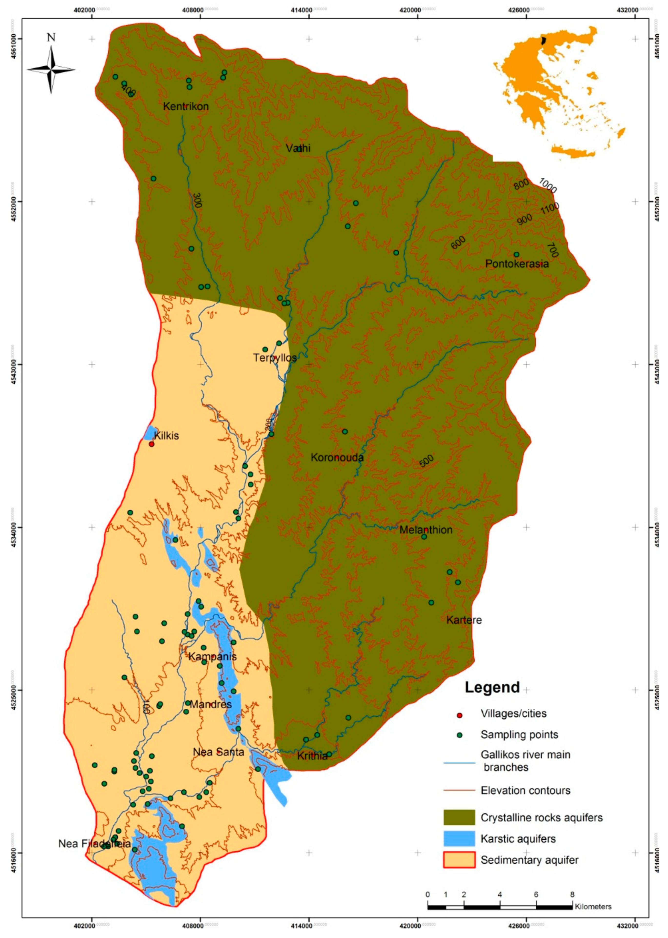
2. Study Area
3. Materials and Methods
3.1. Water Sampling and Analysis
3.2. Multivariate Statistical Analysis
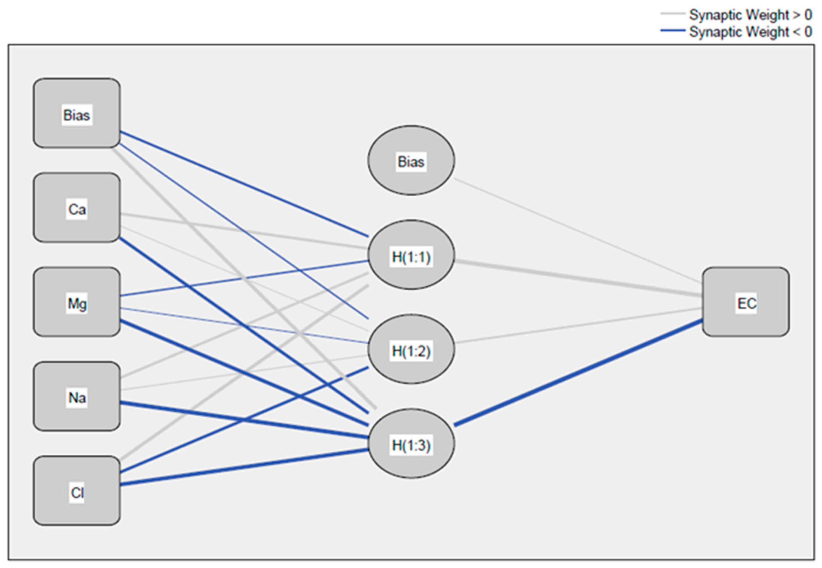
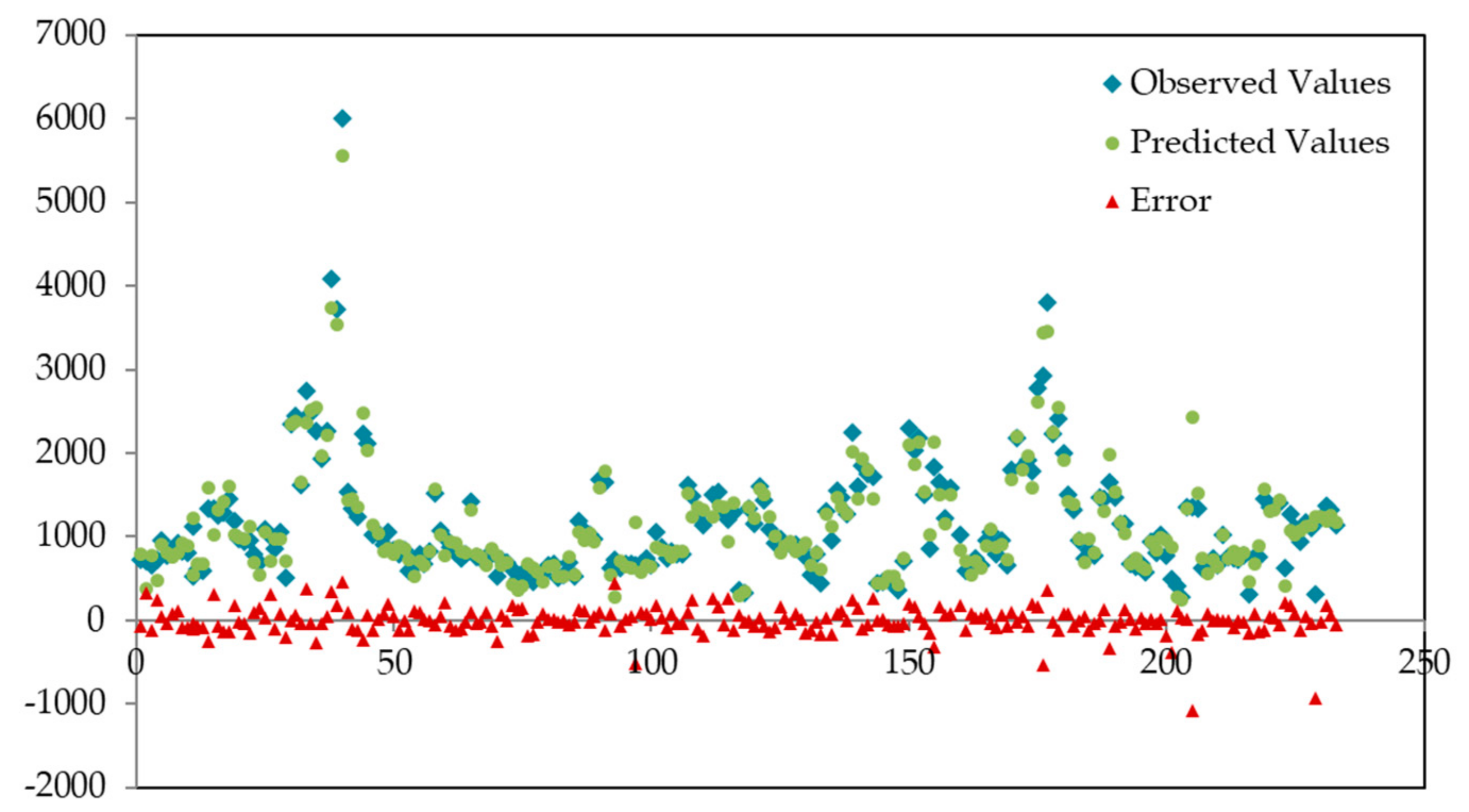
3.3. Artificial Neural Networks
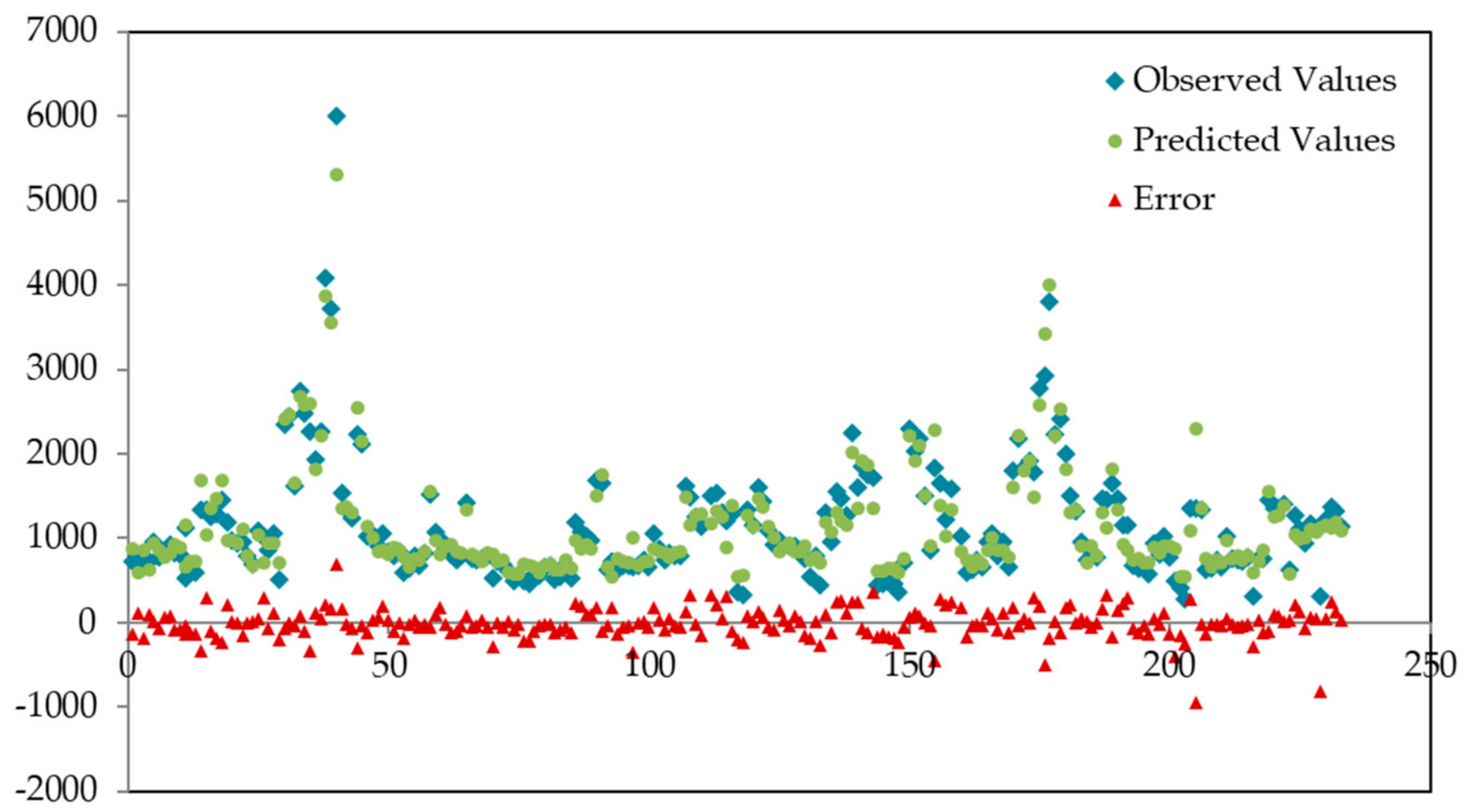
3.4. Multiple Linear Regression
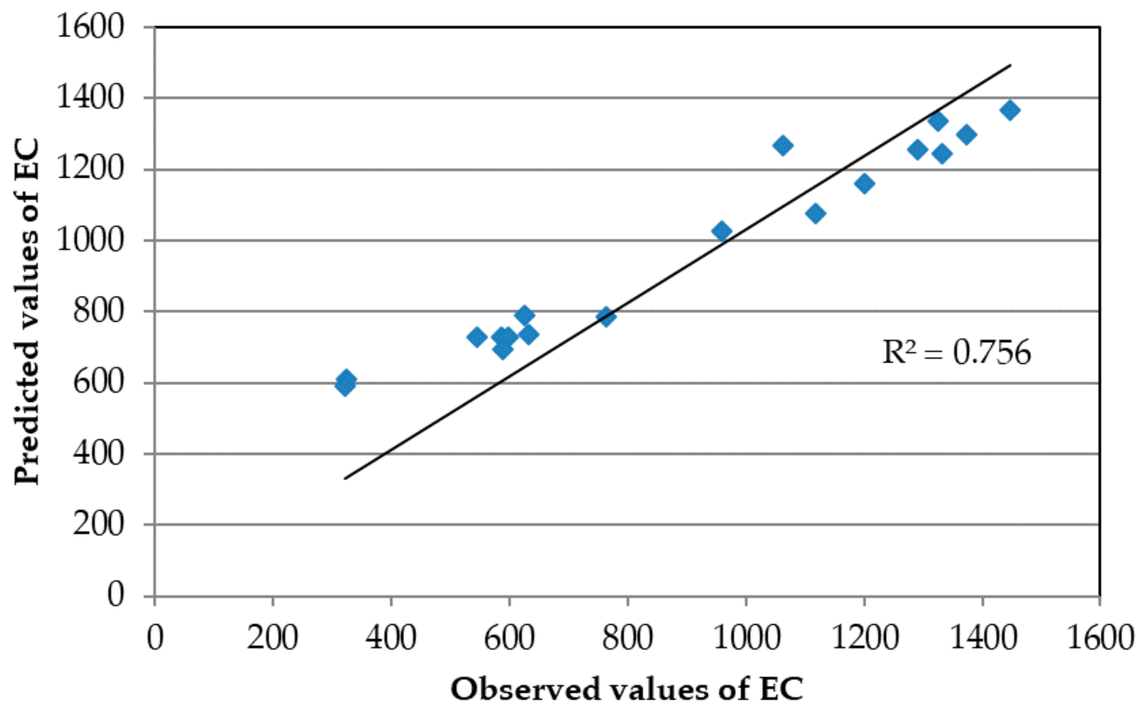
3.5. Performance Evaluation of the Models
4. Results and Discussion
5. Conclusions
Author Contributions
Funding
Institutional Review Board Statement
Informed Consent Statement
Data Availability Statement
Conflicts of Interest
References
- Cay, T.; Uyan, M. Spatial and temporal groundwater level variation geostatistical modeling in the city of Konya, Turkey. Water Environ. Res. 2009, 12, 2460. [Google Scholar] [CrossRef]
- Ehteshami, M.; Biglarijoo, N.; Salari, M. Assessment and quality classification of water in Karun, Dez and Karkheh rivers. J. River Eng. 2014, 2, 23–30. [Google Scholar]
- Napacho, Z.; Manyele, S. Quality assessment of drinking water in Temeke District (part II): Characterization of chemical parameters. Afr. J. Environ. Sci. Technol. 2010, 4, 775–789. [Google Scholar]
- Kristensen, P.; Whalley, C.; Zal, F.N.N.; Christiansen, T. European Waters Assessment of Status and Pressures 2018; European Environment Agency Report; European Environment Agency: Copenhagen, Denmark, 2018. [Google Scholar]
- Qaderi, F.E.; Babanezhad, E. Prediction of the groundwater remediation costs for drinking use based on quality of water resource, using artificial neural network. J. Clean. Prod. 2017, 161, 840–849. [Google Scholar] [CrossRef]
- Chatwell, G.R. Environmental Water Pollution and Control; Anmol Publication: New Delhi, India, 1989. [Google Scholar]
- Kılıçaslan, Y.; Tuna, G.; Gezer, G.; Gulez, K.; Arkoc, O.; Potirakis, S.M. ANN-based estimation of groundwater quality using a wireless water quality network. Int. J. Distrib. Sens. Netw. 2014, 10, 458329. [Google Scholar] [CrossRef] [Green Version]
- Sappa, G.; Ergul, S.; Ferranti, F. Water quality assessment of carbonate aquifers in southern Latium region, Central Italy: A case study for irrigation and drinking purposes. Appl. Water Sci. 2014, 4, 115–128. [Google Scholar] [CrossRef] [Green Version]
- Souissi, D.; Msaddek, M.H.; Zouhri, L.; Chenini, I.; May, M.E.; Dlala, M. Mapping groundwater recharge potential zones in arid region using GIS and Landsat approaches, southeast Tunisia. Hydrol. Sci. J. 2018, 63, 251–268. [Google Scholar] [CrossRef]
- Zanotti, C.; Rotiroti, M.; Fumagalli, L.; Stefania, G.A.; Canonaco, F.; Stefenelli, G.; Prevot, A.S.H.; Leoni, B.; Bonomi, T. Groundwater and surface water quality characterization through positive matrix factorization combined with GIS approach. Water Res. 2019, 159, 122–134. [Google Scholar] [CrossRef] [PubMed]
- Siebert, S.; Burke, J.; Faures, J.-M.; Frenken, K.; Hoogeveen, J.; Döll, P.; Portmann, F.T. Groundwater use for irrigation—A global inventory. Hydrol. Earth Syst. Sci. 2010, 14, 1863–1880. [Google Scholar] [CrossRef] [Green Version]
- Khalil, B.M.; Awadallah, A.G.; Karaman, H.; El-Sayed, A. Application of Artificial Neural Networks for the Prediction of Water Quality Variables in the Nile Delta. J. Water Resour. Prot. 2012, 4, 388–394. [Google Scholar] [CrossRef] [Green Version]
- Ongley, E.D. Water quality management: Design, financing and sustainability considerations-II. Presented at the World Bank’s Water Week Conference: Towards a Strategy for Managing Water Quality Management, Washington, DC, USA, 3–4 April 2000. [Google Scholar]
- Alberto, W.D.; del Pilar, D.M.; Valeria, A.M.; Fabiana, P.S.; Cecilia, H.A.; de los Angles, B.M. Pattern recognition techniques for the evaluation of spatial and temporal variations in water quality, a case study: Suquia river basin (Cordoba–Argentina). Water Resour. 2001, 35, 2881–2894. [Google Scholar]
- Lopez-Chicano, M.; Bouamama, M.; Vallejos, A.; Pulido, B.A. Factors which determine the hydrogeochemical behavior of karstic springs: A case study from the Betic Cordilleras, Spain. Appl. Geochem. 2001, 16, 1179–1192. [Google Scholar] [CrossRef]
- Pereira, H.G.; Renca, S.; Sataiva, J. A case study on geochemical anomaly identification through principal component analysis supplementary projection. Appl. Geochem. 2003, 18, 37–44. [Google Scholar] [CrossRef] [Green Version]
- Kourgialas, N.N.; Karatzas, G.P. A national scale flood hazard mapping methodology: The case of Greece–Protection and adaptation policy approaches. Sci. Total Environ. 2017, 601, 441–452. [Google Scholar] [CrossRef] [PubMed]
- Falah, F.; Rahmati, O.; Rostami, M.; Ahmadisharaf, E.; Daliakopoulos, I.N.; Pourghasemi, H.R. Artificial neural networks for flood susceptibility mapping in data-scarce urban areas. In Spatial Modeling in GIS and R for Earth and Environmental Sciences; Elsevier: Amsterdam, The Netherlands, 2019; pp. 323–336. [Google Scholar]
- Kesikoglu, M.H.; Atasever, U.H.; Dadaser-Celik, F.; Ozkan, C. Performance of ANN, SVM and MLH techniques for land use/cover change detection at Sultan Marshes wetland, Turkey. Water Sci. Technol. 2019, 80, 466–477. [Google Scholar] [CrossRef] [PubMed]
- Singha, S.; Pasupuleti, S.; Singha, S.S.; Singh, R.; Kumar, S. Prediction of groundwater quality using efficient machine learning technique. Chemosphere 2021, 276, 130265. [Google Scholar] [CrossRef]
- Alizadeh, M.J.; Kavianpour, M.R. Development of wavelet-ANN models to predict water quality parameters in Hilo Bay, Pacific Ocean. Mar. Pollut. Bull. 2015, 98, 171–178. [Google Scholar] [CrossRef]
- Lu, F.; Chen, Z.; Liu, W.; Shao, H. Modeling chlorophyll-a concentrations using an artificial neural network for precisely eco-restoring lake basin. Ecol. Eng. 2016, 95, 422–429. [Google Scholar] [CrossRef]
- Nathan, N.S.; Saravanane, R.; Sundararajan, T. Application of ANN and MLR Models on Groundwater Quality Using CWQI at Lawspet, Puducherry in India. J. Geosci. Environ. Prot. 2017, 5, 99–124. [Google Scholar] [CrossRef]
- Rogers, L.L. Optimal Groundwater Remediation Using Artificial Neural Networks and the Genetic Algorithm. Ph.D. Dissertation, Stanford University, Stanford, CA, USA, 1992. [Google Scholar]
- Maier, H.R.; Dandy, G.C. The use of artificial neural networks for the prediction of water quality parameters. Water Resour. Res. 1996, 32, 1013–1022. [Google Scholar] [CrossRef]
- Sandhu, N.; Finch, R. Emulation of DWRDSM using artificial neural networks and estimation of Sacramento river flow from salinity. In North American Water and Environment Congress & Destructive Water; ASCE: New York, NY, USA, 1996; pp. 4335–4340. [Google Scholar]
- Aziz, A.R.A.; Wong, K.-F.V. A neural-network approach to the determination of aquifer parameters. Ground Water 1992, 30, 164–166. [Google Scholar] [CrossRef]
- Abd-Elmaboud, M.E.; Abdel-Gawad, H.A.; El-Alfy, K.S.; Ezzeldin, M.M. Estimation of groundwater recharge using simulation-optimization model and cascade forward ANN at East Nile Delta aquifer, Egypt. J. Hydrol. Reg. Stud. 2021, 34, 100784. [Google Scholar] [CrossRef]
- Tabari MM, R.; Azari, T.; Dehghan, V. A supervised committee neural network for the determination of aquifer parameters: A case study of Katasbes aquifer in Shiraz plain, Iran. Soft Comput. 2021, 25, 4785–4798. [Google Scholar] [CrossRef]
- Isazadeh, M.; Biazar, S.; Ashrafzadeh, A.; Khanjani, R. Estimation of aquifer qualitative parameters in Guilans plain using gamma test and support vector machine and artificial neural network models. J. Environ. Sci. Technol. 2019, 21, 1–21. [Google Scholar]
- Daliakopoulos, I.; Coulibaly, P.; Tsanis, I. Groundwater level forecasting using artificial neural networks. J. Hydrol. 2005, 309, 229–240. [Google Scholar] [CrossRef]
- Mohanty, S.; Jha, M.K.; Kumar, A.; Sudheer, K.P. Artificial Neural Network Modeling for Groundwater Level Forecasting in a River Island of Eastern India. Water Resour. Manag. 2010, 24, 1845–1865. [Google Scholar] [CrossRef]
- Zhu, S.; Hrnjica, B.; Ptak, M.; Choiński, A.; Sivakumar, B. Forecasting of water level in multiple temperate lakes using machine learning models. J. Hydrol. 2020, 585, 124819. [Google Scholar] [CrossRef]
- Hasda, R.; Rahaman, M.F.; Jahan, C.S.; Molla, K.I.; Mazumder, Q.H. Climatic data analysis for groundwater level simulation in drought prone Barind Tract, Bangladesh: Modelling approach using artificial neural network. Groundw. Sustain. Dev. 2020, 10, 100361. [Google Scholar] [CrossRef]
- Diamantopoulou, M.J.; Georgiou, P.E.; Papamichail, D.M. Performance evaluation of artificial neural networks in estimating reference evapotranspiration with minimal meteorological data. Glob. Nest J. 2011, 13, 18–27. [Google Scholar]
- Ghorbani, M.; Aalami, M.; Naghipour, L. Use of artificial neural networks for electrical conductivity modeling in Asi River. Appl. Water Sci. 2017, 7, 1761–1772. [Google Scholar] [CrossRef] [Green Version]
- Mattas, C. Hydrogeological Research of Gallikos Basin. Ph.D. Thesis, Department of Geology, Aristotle University of Thessaloniki, Thessaloniki, Greece, 2009. (In Greek). [Google Scholar]
- Mattas, C.; Anagnostopoulou, C.; Venetsanou, P.; Bilas, G.; Lazoglou, G. Evaluation of Extreme Dry and Wet Conditions Using Climate and Hydrological Indices in the Upper Part of the Gallikos River Basin. Proceedings 2019, 7, 3. [Google Scholar] [CrossRef] [Green Version]
- Mercier, J. Sur l’ existencede l’age de deuxphages regionales de metamorphismealpindans les zones internes des HellenidesenMacedoineCentrale (Grece). Ann. Geol. Des. Pays. Hell. 1966, 20, 1–596. [Google Scholar]
- Mountrakis, D.; Sapountzis, E.; Kilias, A.; Elethfriadis, G.; Christofides, G. Paleogeographic conditions in the western Pelagonian margin in Greece during the initial rifting of the continental area. Can. J. Earth Sci. 1983, 20, 1673–1681. [Google Scholar] [CrossRef]
- Kockel, F.; Walther, H. Die StrymonliniealsGrenzezwischenSerboMazedonischen und Rilla-Rhodope Massiv in Ost-Mazedonian. Geol. Jb. 1965, 83, 575–602. [Google Scholar]
- Kockel, F.; Mollat, H.; Walther, H. Geologie des SerboMazedonischenMassivs und seines mesozoischen Rahmens (Nordgriechenland). Geol. Jb. 1971, 89, 529–551. [Google Scholar]
- Mattas, C.; Voudouris, K.S.; Panagopoulos, A. Integrated groundwater resources management using the DPSIR approach in a GIS environment context: A case study from the Gallikos river basin, North Greece. Water 2014, 6, 1043–1068. [Google Scholar] [CrossRef] [Green Version]
- Official Government Gazette of the Hellenic Republic n.182/v.2/31-01-2014. Available online: http://www.et.gr/idocs-nph/search/pdfViewerForm.html?args=5C7QrtC22wEc63YDhn5AeXdtvSoClrL8P4476sndBGZ5MXD0LzQTLf7MGgcO23N88knBzLCmTXKaO6fpVZ6Lx3UnKl3nP8NxdnJ5r9cmWyJWelDvWS_18kAEhATUkJb0x1LIdQ163nV9K--td6SIuWblVLgGCVMt3UIpyOluks9FzsCB7Qtvn2t1Lb7YCWPL (accessed on 24 August 2021).
- Official Government Gazette of the Hellenic Republic n.3282/v.2/19-09-2017. Available online: http://www.et.gr/idocs-nph/search/pdfViewerForm.html?args=5C7QrtC22wEsrjP0JAlxBXdtvSoClrL8J2n_NccUMzjnMRVjyfnPUeJInJ48_97uHrMts-zFzeyCiBSQOpYnTy36MacmUFCx2ppFvBej56Mmc8Qdb8ZfRJqZnsIAdk8Lv_e6czmhEembNmZCMxLMtUT2iStv6LoLLokjzFTSJwLOlnEGr5bPE7bGxGF96wKi (accessed on 24 August 2021).
- WHO, (World Health Organization). Guidelines for Drinking-Water Quality: Fourth Edition Incorporating the First Addendum, 4th ed.; WHO: Geneva, Switzerland, 2017. [Google Scholar] [CrossRef]
- Mattas, C.; Papachristou, M.; Soulios, G. Assessment of groundwater quality characteristics from the upper part of Gallikos river basin (N. Greece) using factor and cluster analysis methods. In Proceedings of the 10th International Hydrogeological Congress of Greece/Thessaloniki, Athens, Greece, 4–6 October 2014; Voudouris, K., Stamatis, G., Mattas, C., Kaklis, T., Kazakis, N., Eds.; Volume 1, pp. 467–476.
- Mattas, C.; Soulios, G.; Panagopoulos, A.; Voudouris, K.; Panoras, A. Hydrochemical characteristics of the Gallikos river water, Prefecture of kilkis, Greece. Glob. Nest J. 2007, 9, 251–259. [Google Scholar]
- Clesceri, L.S.; Greenberg, A.E.; Trussell, R.R. (Eds.) Standard Methods for the Examination of Water and Wastewater, APHA, AWWA, WPCF, 17th ed.; American Public Health Association: Washington, DC, USA, 1989. [Google Scholar]
- Esmaeili, S.; Moghaddam, A.A.; Barzegar, R.; Tziritis, E. Multivariate statistics and hydrogeochemical modeling for source identification of major elements and heavy metals in the groundwater of Qareh-Ziaeddin plain, NW Iran. Arab. J. Geosci. 2018, 11, 5. [Google Scholar] [CrossRef]
- Machiwal, D.; Jha, M.K. Identifying sources of groundwater contamination in a hard-rock aquifer system using multivariate statistical analyses and GIS-based geostatistical modeling techniques. J. Hydrol. Reg. 2015, 4, 80–110. [Google Scholar] [CrossRef] [Green Version]
- Selle, B.; Schwientek, M.; Lischeid, G. Understanding processes governing water quality in catchments using principal component scores. J. Hydrol. 2013, 486, 31–38. [Google Scholar] [CrossRef]
- Han, Y.M.; Du, P.X.; Cao, J.J.; Posmentier, E.S. Multivariate analysis of heavy metal contamination in urban dusts of Xi’an, Central China. Sci. Total Environ. 2006, 355, 176–186. [Google Scholar]
- Rahman, M.S.; Saha, N.; Molla, A.H. Potential ecological risk assessment of heavy metal contamination in sediment and water body around Dhaka export processing zone, Bangladesh. Environ. Earth Sci. 2014, 71, 2293–2308. [Google Scholar] [CrossRef]
- Garrett, J.H. Where and Why Artificial Neural Networks Are Applicable in Civil Engineering. J. Comput. Civ. Eng. 1994, 8, 129–130. [Google Scholar] [CrossRef]
- Haykin, S. Neural Networks—A Comprehensive Foundations; Prentice-Hall International: Hoboken, NJ, USA, 1999. [Google Scholar]
- Bekas, G.K.; Alexakis, D.E.; Gamvroula, D.E. Forecasting discharge rate and chloride content of karstic spring water by applying the Levenberg–Marquardt algorithm. Environ. Earth Sci. 2021, 80, 1–12. [Google Scholar] [CrossRef]
- Debes, K.; Alexander, K.; Gross, H.M. Transfer Functions in Artificial Neural Networks-A Simulation-Based Tutorial. Brains Minds Media 2005, 2005, 1–11. [Google Scholar]
- Graupe, D. Principles of Artificial Neural Networks, 2nd ed.; World Scientific Publishing Co. Inc.: River Edge, NJ, USA, 2007; ISBN 9812706240. [Google Scholar]
- Chenini, I.; Khemiri, S. Evaluation of ground water quality using multiple linear regression and structural equation modeling. Int. J. Environ. Sci. Technol. 2009, 6, 509–519. [Google Scholar] [CrossRef] [Green Version]
- Ali Khan, M.M.; Umar, R.; Baten, M.A.; Lateh, H.; Kamil, A.A. Evaluation of Groundwater Quality Using Linear Regression Model. J. Appl. Sci. Res. 2012, 8, 251–260. [Google Scholar]
- Ghasemi, J.; Saaidpour, S. Quantitative structure–property relationship study of n-octanol–water partition coefficients of some of diverse drugs using multiple linear regression. Anal. Chim. Acta 2007, 604, 99–106. [Google Scholar] [CrossRef] [PubMed]
- Batabyal, A.K. Correlation and multiple linear regression analysis of groundwater quality data of Bardhaman District, West Bengal, India. Int. J. Res. Chem. Environ. 2014, 4, 42–51. [Google Scholar]
- Bodrud-Dozaa, B.M.; Islam, A.R.M.T.; Ahmed, F.; Das, S.; Saha, N.; Rahman, M.S. Characterization of groundwater quality using water evaluationindices, multivariate statistics and geostatistics in central Bangladesh. Water Sci. 2016, 30, 19–40. [Google Scholar] [CrossRef] [Green Version]
- Neill, S.P.; Hashemi, M.R. Fundamentals of Ocean Renewable Energy: Generating Electricity from the Sea; Academic Press: Cambridge, MA, USA, 2018. [Google Scholar]
- David, M.B.; Del Grosso, S.J.; Hu, X.; Marshall, E.P.; McIsaac, G.F.; Parton, W.J.; Tonitto, C.; Youssef, M.A. Modeling denitrification in a tile-drained, corn and soybean agroecosystem of Illinois, USA. Biogeochemistry 2009, 93, 7–30. [Google Scholar] [CrossRef]
- Craswell, E. Fertilizers and nitrate pollution of surface and ground water: An increasingly pervasive global problem. SN Appl. Sci. 2021, 3, 1–24. [Google Scholar]
- Cirkel, D.G.; Van Beek, C.G.E.M.; Witte, J.P.M.; Van der Zee, S.E.A.T.M. Sulphate reduction and calcite precipitation in relation to internal eutrophication of groundwater fed alkaline fens. Biogeochemistry 2014, 117, 375–393. [Google Scholar] [CrossRef]
- Sharma, M.K.; Kumar, M. Sulphate contamination in groundwater and its remediation: An overview. Environ. Monit. Assess. 2020, 192, 1–10. [Google Scholar] [CrossRef] [PubMed]
- Suresh, K.R.; Nagesh, M.A. Experimental studies on effect of water and soil quality on crop yield. Aquat. Procedia 2015, 4, 1235–1242. [Google Scholar] [CrossRef]
- Lekakis, E.H.; Antonopoulos, V.Z. Modeling the effects of different irrigation water salinity on soil water movement, uptake and multicomponent solute transport. J. Hydrol. 2015, 530, 431–446. [Google Scholar] [CrossRef]
- Oyebode, O.; Stretch, D. Neural network modeling of hydrological systems: A review of implementation techniques. Nat. Resour. Modeling 2019, 32, e12189. [Google Scholar] [CrossRef] [Green Version]
- Jain, A.; Kumar, A.M. Hybrid neural network models for hydrologic time series forecasting. Appl. Soft Comput. 2007, 7, 585–592. [Google Scholar] [CrossRef]
- Gupta, R.; Singh, A.N.; Singhal, A. Application of ANN for water quality index. Int. J. Mach. Learn. Comput. 2019, 9, 688–693. [Google Scholar] [CrossRef]


| Number of Samples | Period | EC (μS/cm) | pH | Ca (mg/L) | Mg (mg/L) | Na (mg/L) | K (mg/L) | HCO3 (mg/L) | SO4 (mg/L) | NO3 (mg/L) | Cl (mg/L) | |
|---|---|---|---|---|---|---|---|---|---|---|---|---|
| 233 | 2004–2005 | minimum | 282 | 6.24 | 12.20 | 11.00 | 12.00 | 0.80 | 85.40 | 1.0 | 0.00 | 1.0 |
| maximum | 6010 | 9.78 | 308.6 | 120.0 | 850.0 | 129.0 | 878.7 | 530.7 | 497.0 | 886.0 | ||
| mean | 1139 | 7.38 | 112.4 | 44.16 | 77.25 | 12.8 | 410.8 | 61.8 | 38.8 | 103.5 | ||
| SD | 686.8 | 0.4 | 56.04 | 21.79 | 84.66 | 16.60 | 117.2 | 62.9 | 62.5 | 135.0 |
| pH | EC (μS/cm) | Ca (mg/L) | Mg (mg/L) | Na (mg/L) | K (mg/L) | HCO3 (mg/L) | SO4 (mg/L) | NO3 (mg/L) | Cl (mg/L) | |
|---|---|---|---|---|---|---|---|---|---|---|
| pH | 1 | −0.075 | −0.093 | −0.063 | 0.063 | 0.135 * | −0.045 | −0.142 * | 0.075 | −0.088 |
| EC | −0.075 | 1 | 0.761 ** | 0.711 ** | 0.853 ** | 0.116 | 0.394 ** | 0.408 ** | 0.343 ** | 0.657 ** |
| Ca | −0.093 | 0.761 ** | 1 | 0.721 ** | 0.450 ** | 0.150 * | 0.436 ** | 0.451 ** | 0.488 ** | 0.525 ** |
| Mg | −0.063 | 0.711 ** | 0.721 ** | 1 | 0.426 ** | 0.085 | 0.532 ** | 0.472 ** | 0.522 ** | 0.498 ** |
| Na | 0.063 | 0.853 ** | 0.450 ** | 0.426 ** | 1 | −0.026 | 0.266 ** | 0.196 ** | 0.096 | 0.464 ** |
| K | 0.135 * | 0.116 | 0.150 * | 0.085 | −0.026 | 1 | 0.139 * | 0.000 | 0.456 ** | 0.144 * |
| HCO3 | −0.045 | 0.394 ** | 0.436 ** | 0.532 ** | 0.266 ** | 0.139 * | 1 | 0.102 | 0.362 ** | 0.188 ** |
| SO4 | −0.142 * | 0.408 ** | 0.451 ** | 0.472 ** | 0.196 ** | 0.000 | 0.102 | 1 | 0.193 ** | 0.510 ** |
| NO3 | 0.075 | 0.343 ** | 0.488 ** | 0.522 ** | 0.096 | 0.456 ** | 0.362 ** | 0.193 ** | 1 | 0.274 ** |
| Cl | −0.088 | 0.657 ** | 0.525 ** | 0.498 ** | 0.464 ** | 0.144 * | 0.188 ** | 0.510 ** | 0.274 ** | 1 |
| Component | Initial Eigenvalues | FACTORS | ||||
|---|---|---|---|---|---|---|
| Total | Cumulative % | 1 | 2 | 3 | ||
| 1 | 4.263 | 42.631 | pH | 0.047 | 0.138 | −0.814 |
| 2 | 1.459 | 57.221 | EC | 0.951 | 0.152 | 0.053 |
| 3 | 1.097 | 68.195 | Ca | 0.719 | 0.401 | 0.259 |
| 4 | 0.961 | 77.802 | Mg | 0.701 | 0.425 | 0.268 |
| 5 | 0.749 | 85.289 | Na | 0.883 | −0.141 | −0.242 |
| 6 | 0.496 | 90.245 | K | −0.069 | 0.760 | −0.182 |
| 7 | 0.388 | 94.123 | HCO3 | 0.391 | 0.466 | 0.047 |
| 8 | 0.314 | 97.258 | SO4 | 0.451 | 0.100 | 0.572 |
| 9 | 0.240 | 99.660 | NO3 | 0.221 | 0.843 | 0.064 |
| 10 | 0.034 | 100.000 | Cl | 0.692 | 0.144 | 0.259 |
| R2 | EF | MAPE (%) | RMSE |
|---|---|---|---|
| Artificial Neural Networks | |||
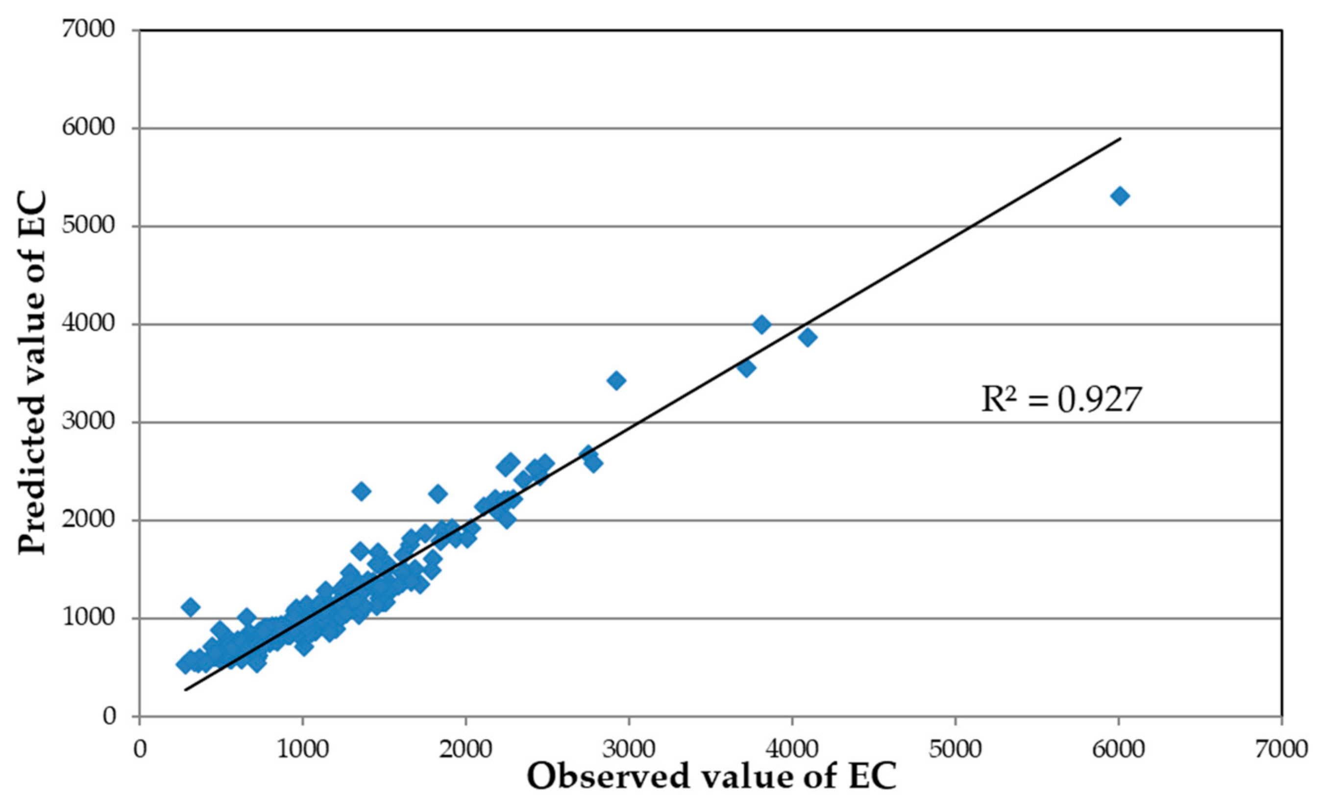
| 0.927 | 0.93 | 14.12 | 175.9 |
| Multiple Linear Regression | |||
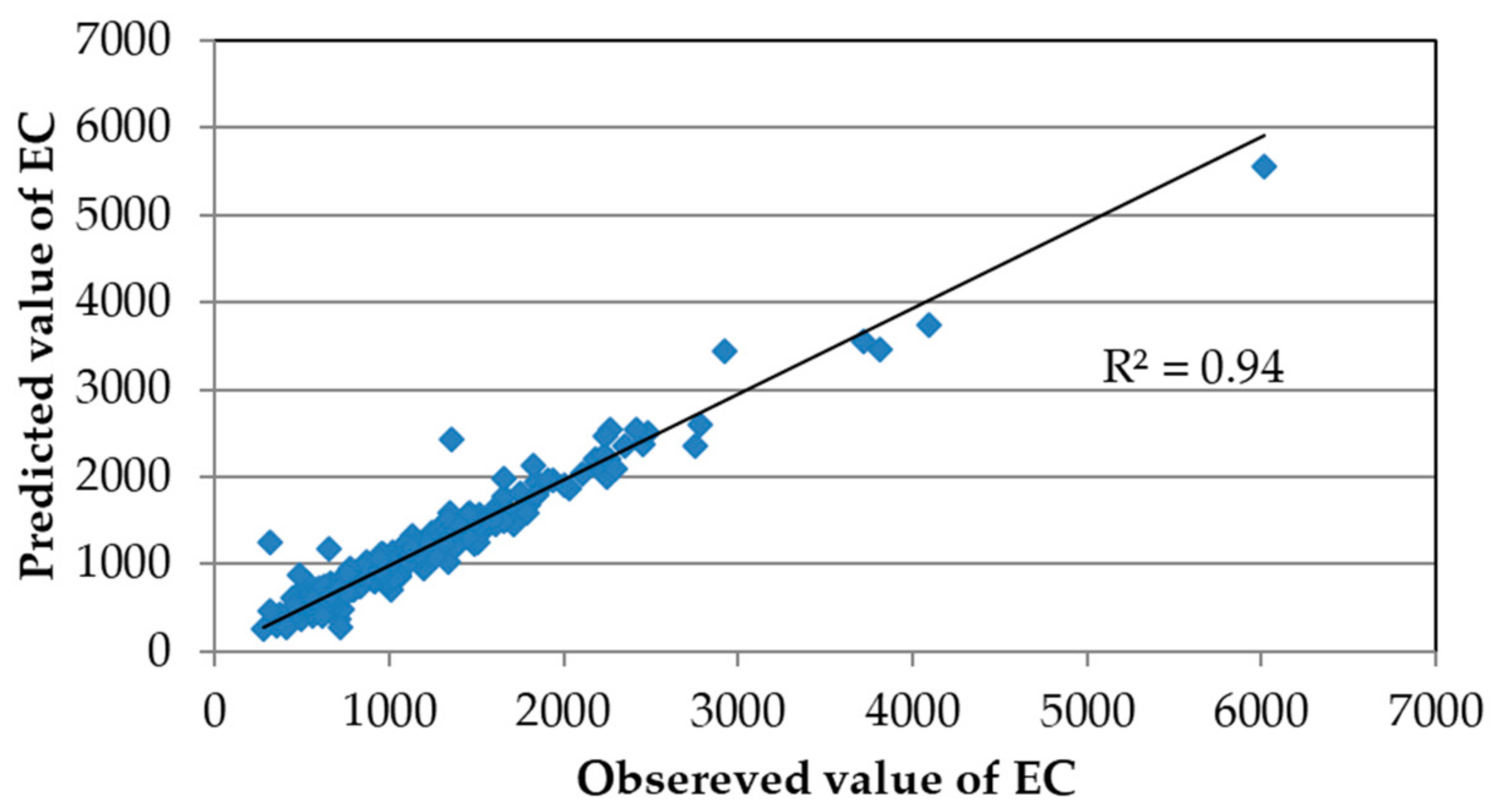
| 0.94 | 0.94 | 12.15 | 168 |
| R2 | EF | MAPE (%) | RMSE |
|---|---|---|---|
| Artificial Neural Network | |||
| 0.75 | 0.979 | 20 | 138.2 |
| Multiple Linear Regression | |||
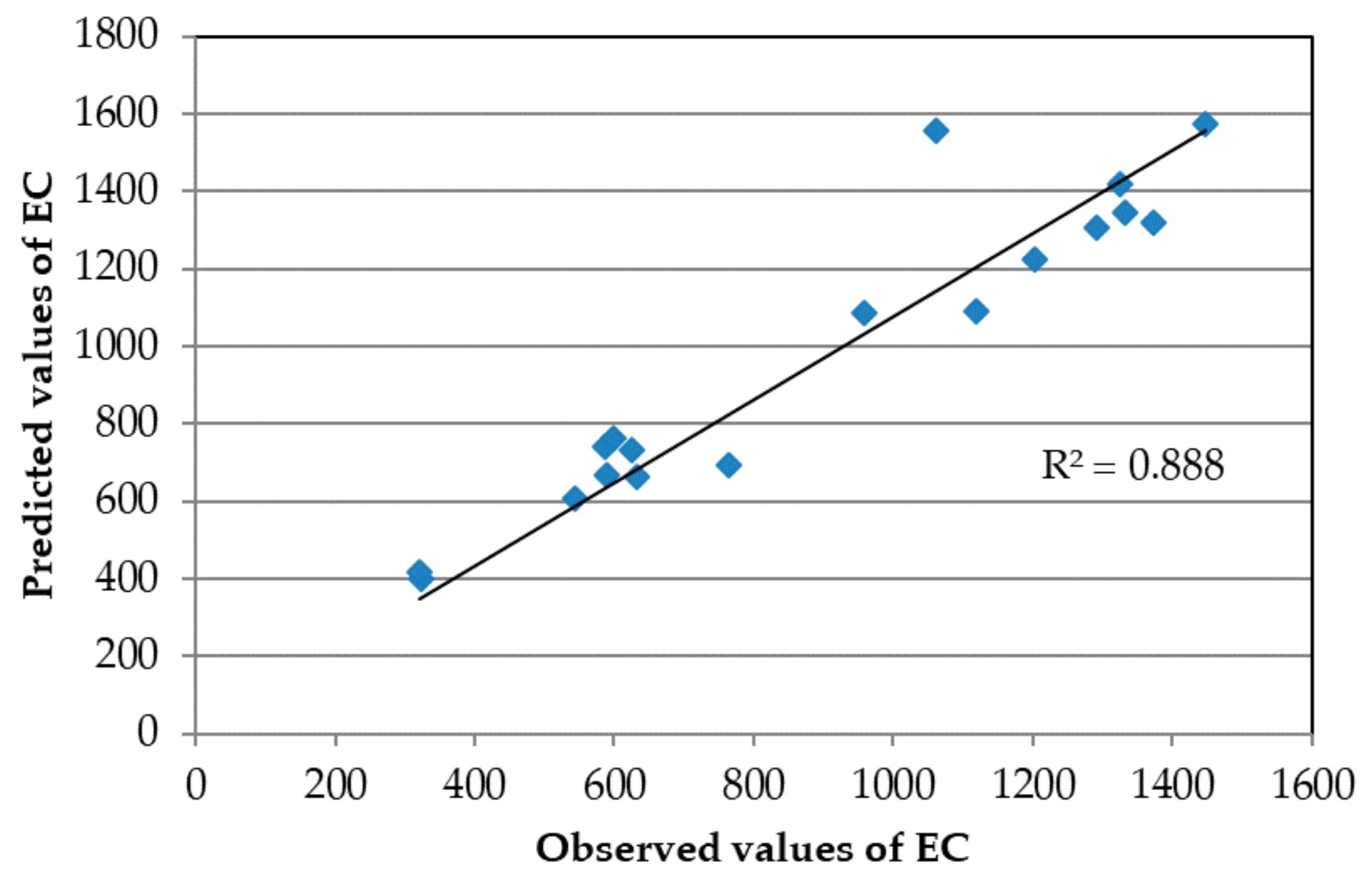
| 0.88 | 0.976 | 13.8 | 145.8 |
Publisher’s Note: MDPI stays neutral with regard to jurisdictional claims in published maps and institutional affiliations. |
© 2021 by the authors. Licensee MDPI, Basel, Switzerland. This article is an open access article distributed under the terms and conditions of the Creative Commons Attribution (CC BY) license (https://creativecommons.org/licenses/by/4.0/).
Share and Cite
Mattas, C.; Dimitraki, L.; Georgiou, P.; Venetsanou, P. Use of Factor Analysis (FA), Artificial Neural Networks (ANNs), and Multiple Linear Regression (MLR) for Electrical Conductivity Prediction in Aquifers in the Gallikos River Basin, Northern Greece. Hydrology 2021, 8, 127. https://doi.org/10.3390/hydrology8030127
Mattas C, Dimitraki L, Georgiou P, Venetsanou P. Use of Factor Analysis (FA), Artificial Neural Networks (ANNs), and Multiple Linear Regression (MLR) for Electrical Conductivity Prediction in Aquifers in the Gallikos River Basin, Northern Greece. Hydrology. 2021; 8(3):127. https://doi.org/10.3390/hydrology8030127
Chicago/Turabian StyleMattas, Christos, Lamprini Dimitraki, Pantazis Georgiou, and Panagiota Venetsanou. 2021. "Use of Factor Analysis (FA), Artificial Neural Networks (ANNs), and Multiple Linear Regression (MLR) for Electrical Conductivity Prediction in Aquifers in the Gallikos River Basin, Northern Greece" Hydrology 8, no. 3: 127. https://doi.org/10.3390/hydrology8030127
APA StyleMattas, C., Dimitraki, L., Georgiou, P., & Venetsanou, P. (2021). Use of Factor Analysis (FA), Artificial Neural Networks (ANNs), and Multiple Linear Regression (MLR) for Electrical Conductivity Prediction in Aquifers in the Gallikos River Basin, Northern Greece. Hydrology, 8(3), 127. https://doi.org/10.3390/hydrology8030127