Article

Susceptibility of Water Resources and Hydropower Production to Climate Change in the Tropics: The Case of Lake Malawi and Shire River Basins, SE Africa

1
Institute for Environmental Science and Geography, Chair for Hydrology and Climatology, University of Potsdam, 14476 Potsdam, Germany
2
Government of the Republic of Malawi, Ministry of Natural Resources, Energy and Mining, Department of Climate Change and Meteorological Services, P.O. Box 1080 Blantyre, Malawi
3
Helmholtz Centre for Environmental Research–UFZ, Brückstraße 3a, D-39114 Magdeburg, Germany
4
Government of the Republic of Malawi, Ministry of Irrigation and Water Developmen Department of Water Resources, Private Bag 390, Capital City, Lilongwe 3, Malawi
*
Author to whom correspondence should be addressed.
Hydrology 2020, 7(3), 54; https://doi.org/10.3390/hydrology7030054
Submission received: 22 June 2020 / Revised: 29 July 2020 / Accepted: 5 August 2020 / Published: 7 August 2020

Abstract

:
The sensitivity of key hydrologic variables and hydropower generation to climate change in the Lake Malawi and Shire River basins is assessed. The study adapts the mesoscale Hydrological Model (mHM) which is applied separately in the Upper Lake Malawi and Shire River basins. A particular Lake Malawi model, which focuses on reservoir routing and lake water balance, has been developed and is interlinked between the two basins. Climate change projections from 20 Coordinated Regional Climate Downscaling Experiment (CORDEX) models for Africa based on two scenarios (RCP4.5 and RCP8.5) for the periods 2021–2050 and 2071–2100 are used. An annual temperature increase of 1 °C decreases mean lake level and outflow by 0.3 m and 17%, respectively, signifying the importance of intensified evaporation for Lake Malawi’s water budget. Meanwhile, a +5% (−5%) deviation in annual rainfall changes mean lake level by +0.7 m (−0.6 m). The combined effects of temperature increase and rainfall decrease result in significantly lower flows in the Shire River. The hydrological river regime may change from perennial to seasonal with the combination of annual temperature increase and precipitation decrease beyond 1.5 °C (3.5 °C) and −20% (−15%). The study further projects a reduction in annual hydropower production between 1% (RCP8.5) and 2.5% (RCP4.5) during 2021–2050 and between 5% (RCP4.5) and 24% (RCP8.5) during 2071–2100. The results show that it is of great importance that a further development of hydro energy on the Shire River should take into account the effects of climate change, e.g., longer low flow periods and/or higher discharge fluctuations, and thus uncertainty in the amount of electricity produced.

1. Introduction

Climate is changing around the world and one of the sectors being affected most is water resources. The hydrological effects of climate change vary from region to region. For instance, altered rates and different timing of river flows are observed in high latitudes due to snow melting and increases in precipitation [1], while decreased flows are also noticeable in the mid-latitudes and dry tropics [2]. These climate change impacts on water resources have not spared the African continent, where the frequency and intensity of droughts is rising [3]. Fourteen countries are already under water stress as water availability has decreased 2.8 times between 1970 and 1995 [4]. In southern Africa, the highly ranked water-stressed countries are Namibia, South Africa, Lesotho, Botswana and Eswatini, while the rest of the countries in the region are rated medium or low [5]. Extreme hydrological events, such as floods and droughts, are also common in Africa, and these are expected to increase under climate change, worsening the water situation in the continent [4,6]. Southern Africa is one of the most vulnerable greater regions to climate change [7] and, if the recent rate of change persists into the future, the impact on water resources will be enormous [8].
A particular example of a very important but vulnerable hydro-system in the tropics is Lake Malawi and its river basin. As the fifth/ninth largest freshwater lake in the world (in terms of water volume/surface area), it is the key water resource and reservoir for hydropower generation on the Shire River, which originates at the only southern outlet of the lake. The capacity installed and electricity generated at the hydropower plants in Malawi account for 80.2% and 98%, respectively, of the country’s total electricity power [9]. Lake level fluctuations affect the power production on the Shire River, for example, the below normal rainfall seasons of 2014/2015 and 2015/2016 resulted in falling lake water levels and reduced river flows, which decreased the power production by more than 50% [10]. Between 1915 and 1935, the outflow from the lake into the Shire River totally ceased [11], which nowadays would lead to a complete failure in energy supply. During the last four decades (1970–2013), droughts in the greater Lake Malawi Basin have increased in terms of duration, severity and area proportion due to both a decrease in precipitation and an increase in temperature (leading to increased evapotranspiration), which have led to declining lake levels in Lake Malawi [12]. Future climate projections from various studies indicate a temperature increase in the southern Africa region from 2 to 5 degrees Celsius until 2100 [8,13,14,15,16]. Though there is uncertainty in the magnitude and direction of mean precipitation projection in the region, many studies based on climate projections have suggested decreasing trends until 2100 [8,17,18].
Hydropower will maintain its position as the main source of electricity in the short to medium term in Malawi as compared to other energy sources. There are plans to invest in even more hydropower stations along the Shire River to meet the future energy demands [19,20,21]. However, with reference to the recent increasing trends in both meteorological and hydrological droughts in Malawi [12], future changes in climate may further reduce river flows [4,6,22] and thus affect the hydropower production, which puts the energy supply in Malawi under threat.
Although hydropower is the key energy source in Malawi, there are only a few studies that have quantified the impacts of climate change on hydropower generation, (e.g., [23]). Most climate impact studies on the Southern and Southeastern Africa regions focussed on water resources in general [6,8,24,25,26], agriculture [27,28,29], health [30] and multiple other sectors including energy, the environment and disasters [4,31,32]. For the Zambezi River, reduced hydropower production has been projected for the future until the 2080s based on three General Climate Models (GCMs) [22,33]. In Malawi, reduced hydropower generation at the Lujeri Micro-Hydropower Scheme in southern Malawi during 1980–2011 was attributed to increased temperature [34]. The decrease in Lake Malawi’s level that would potentially lead to no outflow from the lake was identified for the period 2021–2050 based on 11 out of 30 climate models [31] and up to 2100 based on a single model [25]. This would have serious consequences for hydropower production.
So far, however, the impacts of possible changes in future climate on streamflow and hydropower productivity on the Shire River have rarely been investigated despite their crucial relevance for electricity supply in Malawi. This study (i) examines the sensitivity of the hydrological system of Lake Malawi and its basin, as well as of the Upper Shire River Basin, towards changes in key climate parameters based on dynamical hydrological modeling; (ii) estimates potential impacts of future climate change on the hydrological system by means of so-called scenario-neutral response surfaces and based on a 20-model ensemble of Regional Climate Models (RCMs); and (iii) illustrates the impacts of changes in the hydrological system on future hydropower generation in Malawi. The study is led by the following questions:
  • How sensitive are lake levels and discharge to variations in precipitation and temperature (potential evapotranspiration and lake evaporation) in the Lake Malawi Basin (including the lake) and Shire River Basin?
  • What are the impacts of future climate change projections on the water budgets of the Lake Malawi Basin and Shire River Basin?
  • How do these impacts translate into changes in hydropower productivity and reliability?

2. Study Area and Data

2.1. Study Area

Lake Malawi is located in southeastern Africa along the Great Rift Valley. It is one of the southernmost lakes (Figure 1b) and its north−south extension is approximately 560 km, the maximum width is 75 km and the average depth is 292 m. The catchment area is 125,500 km² including the lake surface area, which is about 29,600 km². The lake has several inflows and only one outlet in the south; the Shire River, which originates at Mangochi (Figure 1a). The Shire River, downstream of Mangochi, is 401 km long, has a catchment area of 23,500 km², and joins the Zambezi River in Mozambique as its most downstream tributary (Figure 1b). The middle Shire, characterized by deep gorges with steep slopes, is 80 km long and is where hydropower generation takes place (Figure 1a). The hydraulic gradient of 370 m provides an important potential for hydropower generation [11], and currently seven hydropower plants (Table 1) are installed that contribute 98% of installed hydroelectrical power in Malawi [9].
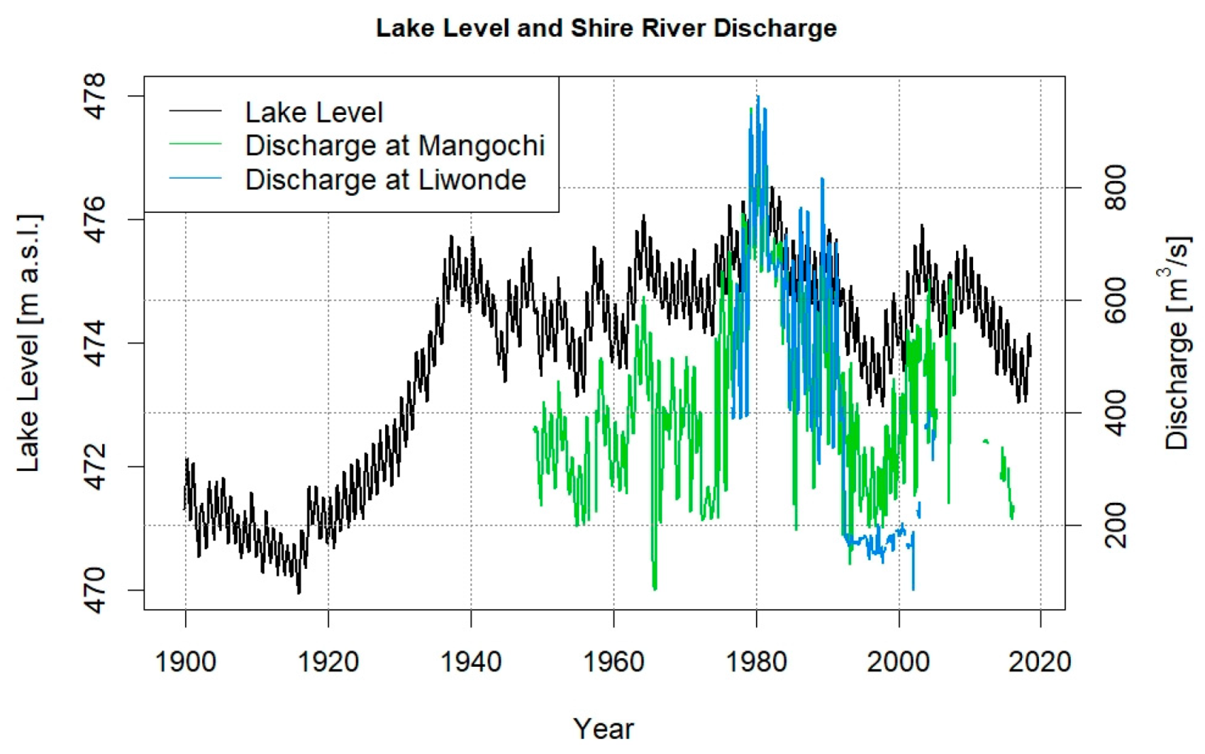
Lake level variability highly affects river discharge in the upper Shire River (Figure 2). For the full utilization of the installed hydropower capacity, a steady flow of ≥170 m3/s at gauge Liwonde (Figure 1a) is required [11]. In terms of runoff seasonality, high flows occur from January to May and the lowest flows usually occur during October to December [11]. This is closely connected to the hydro-meteorological conditions in Malawi. Located in the tropics, the climate in Malawi depends on the inter-tropical convergence zone, the sub-tropical high-pressure belt further south, and its topography. There is a pronounced rainfall gradient in annual rainfall from the north (>1400 mm) to the south (<900 mm) [12]. The country is characterized by a prominent warm summer and rainy season between October and April [35,36], with monthly rainfall depths on average above 200 mm and an average air temperature varying between roughly 26 and 28 °C and a dry and cool winter season between June and September with very little rainfall (between 0 mm and 20 mm/month) and average an air temperature between 21 and 25 °C (Figure 1c).
The dominant land cover in the Lake Malawi and Shire River basins is cultivated land. In 2005, cultivated land covered 33.7%, while forest area coverage was at 24.3%, savanna woodlands and shrubs were at 19.9% and the rest (22.1%) was covered by water [37]. Land cover is changing in the basin towards more cultivated land and less savanna woodlands and forest [38]. In the upper Shire River catchment, agricultural land increased by 18% from 1989 to 2002 [38], while forest cover in the Lake Malawi Basin decreased from 64% in 1967 to 51% in the early 1990s [39].

2.2. Data

Monthly lake level and daily lake outflow data sets are from the Department of Water Resources in Malawi and cover the periods from 1899 to 2018 and 1948 to 2014, respectively. Daily temperature and mean relative humidity data sets are from the Climatic Research Unit (CRU) at the University of East Anglia (http://www.cru.uea.ac.uk/data) [40].
Rainfall data for 65 locations is obtained from the Department of Climate Change and Meteorological Services in Malawi for the period 1960s to 2013. Gridded 0.5° Global Precipitation Climatology Centre (GPCC) data from the German Weather Service (DWD) [41] complement rainfall data on the Tanzanian and Mozambiquan sides of the Lake Malawi Basin. It has been shown that GPCC rainfall data represent rainfall characteristics in this region reasonably well [42]. Point data are gridded into a 0.5-degree resolution using the Inverse Distance Weighted (IDW) method by Shepard [43], which has been applied successfully by many, including Bashir and Fouli and Pai et al. [44,45].
For future climate (precipitation and temperature), the Coordinated Regional Climate Downscaling Experiment (CORDEX) data for Africa are used, i.e., in order to reduce the inherent uncertainty of GCMs and RCMs, we did not to rely on the results of a single climate model but instead used the output of the model ensemble of the CORDEX Africa consortium. This is a dynamically downscaled data set [46] from Coupled Model Inter-comparison Project 5 (CMIP5) General Climate Models (GCMs) using Regional Climate Models (RCMs) at about a 50 km (0.44°) resolution. This data set has been found to simulate the historical rainfall and temperature variations over Africa satisfactorily [47,48,49]. In this study, only models with full simulations for both Representative Concentration Pathway 4.5 (RCP4.5) and RCP8.5 from 1976 to 2100 are used for easy comparability. RCP8.5 is almost a business as usual scenario [50], while RCP4.5 is the moderately controlled scenario. RCP4.5 has moderate population growth and economic growth, while the forest area increases as the crops and grassland decline [51]. Future scenarios are grouped into two periods, 2021–2050 (near future) and 2071–2100 (far future). For each period and concentration pathway considered, the simulations of an ensemble of 20 GCM–RCM combinations from CORDEX Africa are used. Table 2 provides a full overview about the various linkages of ten GCMs (columns) and five RCMs (rows) leading to the ensemble of 20 combinations from five centers. Abbreviations for the centers are described in the caption of Table 2. CORDEX data are accessed through the Earth System Grid Federation (ESGF) at https://cordex.org/data−access/esgf/.
The digital elevation model (DEM) and its derivatives, which are mainly used for initializing the river network in the mesoscale Hydrological mMdel (mHM), are taken from HydroSHEDS (https://hydrosheds.org/), while the soil database is from SOILGRIDS (https://soilgrids.org/). Land cover maps and geological information are obtained from GLOBCOVER (http://due.esrin.esa.int/page_globcover.php) and the Global Lithological Map (GLIM, https://www.geo.uni−hamburg.de/en/geologie/forschung/geochemie/glim.html), respectively.

3. Methods

3.1. Modeling Strategy

The investigation of potential climate change impacts on the hydrological system of the Lake Malawi Basin and Shire River Basin is based on a cascade of hydrological models (Figure 3). This cascade consists of (i) a hydrological model upstream of the lake, the Upstream Lake Malawi Basin Model (ULMBM), i.e., for all rivers flowing into the lake in order to simulate dynamic lake inflow, (ii) a lake model that calculates the lake’s water budget, including lake level changes and outflow variations (Lake Malawi Model, LMM) and (iii) a hydrological model for the upper and middle Shire River to simulate river discharge of this river system (Shire River Model, SRM) that can be translated into hydropower productivity (HPP). The hydrological models are realized by adjusting the mesoscale Hydrological Model (mHM) for the respective catchments (details in Section 3.2). The SRM takes the outflow computed from the LMM (details in Section 3.3) as inflow into its upper boundary, i.e., the origin of the Shire River. All parts of this model cascade are calibrated and tested for independent time periods. The sensitivity of the hydrological system of the Lake Malawi and Shire River basins, as well as potential climate change impacts on hydropower productivity, are assessed by systematically varying the meteorological inputs, i.e., precipitation and temperature. The following subsections describe the individual components of the model cascade and the sensitivity experiments in more detail.

3.2. Mesoscale Hydrological Model (mHM)

The mesoscale Hydrological Model (mHM) is a spatially distributed, partly process-based model that treats grid cells as unique hydrological units. It comprises hydrological processes such as interception, snow accumulation and melting, infiltration, soil water dynamics, groundwater recharge and storage. The generated discharge of a model cell consists of direct runoff, baseflow and slow and fast interflow, which, after aggregating its components, is routed through the model domain using the Muskingum−Cunge flood routing algorithm [52,53]. By using the multiscale parameter regionalization technique [54,55], the mHM directly accounts for the sub-grid variability of the physiographic characteristics. In the mHM, the model parameters are estimated in a preliminary step at the lowest possible input resolution of the physiographic variables. In case of the ULMBM and SRM, these grids are 1/128 degrees × 1/128 degrees (or ~867 m × 867 m). In step two, effective parameters at mode a resolution of 0.5 degrees × 0.5 degrees are estimated by applying particular upscaling operators. This technique makes the mHM scale- and location-independent because it connects effective parameters to physiographical inputs [55]. Having such a scalability feature means better control over equifinality of the model with a more restrained parameter space. Plus, the mHM also has a satisfactory performance over a wide range of catchments sizes (4 to 530,000 km2) and contrasting climatic regimes (Europe, Asia, North America, South America, Australia and Africa (West and Horn of Africa) [54,56,57,58,59,60]), hence chosen as the hydrological model for our analysis.
We apply the mHM at a 0.5-degree (~55 km) grid resolution at daily time steps on the Lake Malawi and Shire River Basins. The model is adjusted to the catchment upstream of Lake Malawi (ULMBM; Figure 3) to simulate daily inflow into the lake, and to the catchment of the upper and middle Shire River (SRM; Figure 3) to simulate discharge, from which hydropower productivity can be derived. Lake inflow is simulated for 33 rivers (red points around the lake in Figure 1a). Due to the rather coarse spatial resolution opted for the ULMBM, some inflow points fall into the same grid cell, so these points are aggregated, which results in a total of 23 inflow points. Attributable to the best daily (continuous) discharge data availability (in terms of temporal coverage and data quality), the calibration of the ULMBM is performed at Zayuka gauge on the Luweya River (blue point in Figure 1a) for the period November 1988 to October 1995. The calibration for the SRM is performed at Liwonde gauge, which provides the comparatively good hydrological data integrity in this section for the period November 1985 to October 1991. The model calibration uses the Dynamical Dimensioned Search (DDS) [61], which is a global optimization algorithm for the calibration of multiple-parameter models. DDS finds best fit parameter sets based on a user-defined maximum number of model calls. We use 3000 model runs to separately calibrate the ULMBM and SRM. The Kling−Gupta Efficiency (KGE) [62], which combines the bias, the correlation and the variability between simulated and observed discharge, is used as the objective function. The KGE is given as:
K G E = 1 ( r 1 ) 2 + ( β s β o 1 ) 2 + ( s o ¯ ¯ 1 ) 2
where r is the correlation coefficient, s o ¯ ¯   is the bias ratio, in which s ¯ and o ¯ are the mean values for simulated and observed values, respectively, β s β o   is the variability ratio between simulated and observed discharge, with β as the coefficient of variation, where β s = δ s / s ¯ and β o = δ o / o ¯     , and δ s and δ o are the standard deviations for simulated and observed data, respectively. The combination of the three parameters provides a good insight into the model performance, as temporal discharge dynamic is captured by r and the flow duration curve is captured by the bias and variability terms (Kling et al. 2012). In turn, KGE = 1 represents the best model, which means all the three parameters r, β s β o and s o ¯ ¯ are unity. The calibrated ULMBM and SRM are tested for the independent time periods November 1985–October 1988 and November 1977−October 1982, respectively.

3.3. Lake Malawi Model (LMM)

For our study area, lake water budget plays a prominent and crucial role within the whole hydrological system. Therefore, we develop a model that accounts for the water balance including the lake level and outflow dynamics of Lake Malawi. The lake model applies a reservoir routing method, which is basically based on the lake water balance dynamic and an empirical relationship between lake level and outflow volume. The basic lake water balance equation reads as follows:
d S L d t = P L + Q i n E L Q o u t
where d S L d t is the change in storage that can be translated into lake level change and groundwater exchange. Groundwater exchange is, however, neglected due to an unavailability of adequate data in this area [25]. Qin and Qout are lake inflow and outflow, respectively, PL is the precipitation on the lake and EL is the water loss due to lake evaporation.
Based on Equation (2), we estimated daily water fluxes within the lake reservoir. Daily Qin is dynamically simulated by the ULMBM (c.f. Section 3.1), and daily PL is taken from the interpolated daily precipitation grids described in Section 2.2. Lake evaporation (EL) at daily time steps is estimated using the Penman formula for open water bodies [63].
The Penman formula for open water evaporation is based on energy balance on the Earth’s surface. The formula, modified by the Food and Agriculture Organisation (FAO), assumes heat flux density into the water to be zero at daily periods so that the final version is composed of a radiation term (a) and a wind term (b) [64].
E L = c [ Δ Δ + γ R a + γ Δ + γ   2.7 f ( u ) ( e a e d ) ] ( a )                                     ( b )
The radiation term (a) is comprised of R a , which is the equivalent net radiation (incoming minus reflected solar radiation minus the budget of long wave radiation), and Δ is the slope of the saturation vapor pressure curve [kPa °C−1], estimated using
Δ = 4098 [ 0.61 e x p ( 17.27 T T + 237.3 ) ] ( T + 237.3 ) 2
and T [°C] is average temperature and γ is a psychrometric constant (we applied a constant value of 0.67 kPa °C−1). The wind term (b) includes a function f(u) which is estimated by 1 + 0.864 u 2 and u 2 is the surface wind speed at 2 m above ground. The term (eaed) is the vapor pressure deficit, as e a is the saturated vapor pressure at temperature T a and ed is the prevailing vapor pressure. Finally, c is a dimensionless adjustment factor [64]. The variation of wind speed over monthly periods is relatively small so that wind speed is assumed to be steady at 2 m/s, which is the average wind speed found at over 2000 weather stations around the world [64]. Evaporation from the lake plays a crucial role within the hydrological system of the lake since previous estimates for Lake Malawi report only 16.3% to 19.5% of the annual water received into the lake is transposed to outflow, the rest is lost by lake evaporation [65,66,67].
Referring to Kumambala and Ervine [25], the lake outflow at Mangochi (Qout) is a power law function of lake level that refers to the following relationship:
Q o u t = 30.285 ( L 470.8 ) 1.9145
where L − 470.8 is the effective lake level above the crest of the Shire riverbed sill at the lake outlet, i.e., 470.8 m a.s.l., which indicates the level at which no outflow into the Shire River occurs. The factor and the exponent are calibrated and adjusted based on outflow and lake level data to best match lake outflow and observed discharge at Mangochi, the gauge at the outlet of the lake (R² = 0.97) [25].
In the late 1960s, a barrage was installed at Liwonde to control discharge into the Shire River within the lake level range of between 473.2 and 475.3 m a.s.l. Lake outflow (in m3/s) is regulated as follows [11]:
Q o u t = { Q o u t ,   i f   L > 475.32   m   a . s . l . 237 ( L 471.37 ) 411 ,     i f   473.82 < L < 475.32   m   a . s . l . 170 ,   i f   473.22 < L < 473.82   m   a . s . l . Q o u t ,   i f   L < 473.22   m   a . s . l .
The developed lake model takes these operation rules into account, although observed discharge data at Liwonde suggest that these rules have not always been completely followed [67] (see Figure 2). This agrees with Shela [11], who indicated that a temporal rule was introduced following the massive 1992 drought to control water flow between 155 to 200 m3/s whenever the lake level is above 473.22 m a.s.l., otherwise the gates are opened.
The dynamic estimation of lake level (changes), based on lake inputs (river inflows and rainfall) and outputs (Shire River outflow and water loss due to evaporation), is crucial for the water budget of the lake. The lake model has been tested for the period 1976–2013 by comparing simulated lake level and lake outflow with observations. The dynamic lake model has been implemented in R [68].

3.4. Estimation of Hydropower Production

Hydropower production (HPP) is a function of gravitational acceleration g, efficiency of the system μ, net hydraulic head h of the power station, density of water ρ and river discharge Q.
H P P = g ρ μ h Q
As g and ρ are constants and μ and h are known and assumed constant for each individual power station (see Table 1), Q is the missing variable which we infer from the simulations of the SRM (Figure 3). The power calculated here is an ideal, i.e., power production breaks or reduction due to, e.g., maintenance or repair works at the power stations are not considered. The energy production is estimated at the three main power station groups on the Shire River: at Nkula, representing Nkula hydropower stations A and B, at Tedzani (I, II and III) and at Kapichira hydropower station (I and II) (see Table 1). As Nkula and Tedzani are located only 7 km apart from each other and no tributaries enter into the Shire in this section, the energy of those two groups is calculated with the same river discharge Q at this river stretch. The production of all seven stations is then added to obtain the overall energy production on the Shire River. The total installed hydropower on the Shire River at all seven hydropower stations is 346.3 MW, which yields a maximum daily production of 8304 GWh per day (Table 1), assuming the turbines are running with full capacity and the efficiency of the system is 90% (μ = 0.9). To fully utilize this capacity, a firm flow of ≥ 170 m3/s at Liwonde is required [11].

3.5. Sensitivity Analysis and Response Surfaces

To illustrate the sensitivity of the overall Lake Malawi/Shire River hydro-system towards variations in the most important hydro-climatological drivers, we systematically perturb the input variables temperature and precipitation, and run the whole model cascade with these perturbed time series. The perturbation is applied to reference period of 1976 to 2005 at daily time steps. Observed daily time series of the crucial meteorological variables temperature (To) and precipitation (Po) are linearly scaled within a given range of allowed change:
T ( i ) T o ( i ) + X t
P ( i ) P o ( i ) X p
where Xt and Xp are the perturbation factors which incrementally scale the observed input data (additive for temperature; multiplicative for precipitation) and i indicates the daily time step. Daily temperature time series are systematically perturbed by up to +5 °C with +0.5 °C increments, leading to ten different model realizations. Precipitation time series are perturbed within −20% to +30% with 5% increments, also leading to ten different model realizations. We then compare the simulated time series generated with the perturbed input data to the reference simulation that is generated by the original input data (To and Po). This sensitivity test is applied to all the three model parts, the ULMBM, LMM and SRM (Figure 3), to highlight the sensitivity of the hydrological system towards changes in the hydro-meteorological drivers. The target variables of the simulations are lake level, lake outflow and Shire River flow dynamics. By linearly scaling the temperature and precipitation, the monthly, seasonal and annual cycles are conserved.
To estimate the potential impacts of climate change (i.e., changes in temperature and precipitation) on lake level, discharge and hydropower productivity in the upper and middle Shire River, we generate so-called response surfaces. Response surfaces are generated by summarizing the response of lake level and discharge towards changes in the climate system estimated by a systematic sensitivity analysis in a two-dimensional matrix. In this study, the entire hydrological model chain (Figure 3) is run with all possible combinations of perturbed daily temperature and precipitation time series generated for the sensitivity analysis (Equations (8) and (9)), and the result of each combination (i.e., the mean impact) is plotted as one single realization (i.e., one pixel) of possible climate change impacts in a two-dimensional domain (i.e., the response surface with 11 × 11 = 121 realizations, thus including the reference pixel, i.e., the realization with non-perturbed, original input data). This so-called scenario-neutral approach was introduced by Prudhomme et al. [69] and has been applied for various purposes [1,70]. In that way, this approach differs from top-down approaches that apply an ensemble of (locally adjusted) GCM–RCMs as inputs into the hydrological model. Still, the spread and the mean of an ensemble of climate projection can be visualized by overlaying the climate change signals from the GCM–RCMs over the response surfaces, which provides an intuitive illustration of the uncertainties of the impact response: the wider the spread, the larger the uncertainties. In turn, the response values that are covered by the spread of the ensemble show the range of possible impacts [71].
In this study, we apply simple linear scaling to the meteorological input data, as shown in Equations (8) and (9), although this neglects possible modifications of the temporal structure of the input and response data due to climate change [1,70]. This limitation is similar to the criticism raised against delta change approaches for statistical downscaling in top-down approaches [72]. However, since we are interested in the mean long-term impacts of climate change on runoff and hydropower productivity, simple linear scaling is a reasonable approach for the generation of the response surfaces. The spread and the mean of the ensemble climate projections (cf. 2.2) are overlaid on the response surfaces to indicate the physically projected climate change in the greater Lake Malawi Basin/Shire River Basin.

4. Results

4.1. Calibration and Verification of the Hydrological Model Chain

The three components of the hydrological model chain are calibrated and verified independently. Each calibration includes a warm-up period of two years for stabilizing the soil moisture in the model. We use seven years (1988–1994) and six years (1985–1990) for the calibration of the mHM for the ULMBM and SRM, respectively. In comparison, the mHM has been successfully applied in the existing literature with calibration periods ranging from 3 to 20 years [54,55,56,57,73,74].
Figure 4 presents the hydrographs simulated by the ULMBM and SRM in comparison with runoff observations for the respective calibration and verification periods, including the KGE estimates which are used as a goodness of fit measure. Regarding the ULMBM, which simulates inflow into Lake Malawi, the calibrated model slightly overestimates low flows but matches the seasonal cycle and peak flows rather well. The skill determined by the KGE for the calibration period is 0.8. Applying the calibrated ULMBM to a three-year verification period (1985–1988), the skill drops by only 3.75% (KGE = 0.78). Here, the model partly underestimates high flows but matches low flows relatively well. In turn, some water inflow into the lake, e.g. by groundwater, might be missed by the model. However, the volumetric bias is low (7.0%), and this rarely affects the simulation of lake level dynamics (see Figure 5 upper panel).
The calibrated SRM, which takes outflow from the lake model as input, is able to reproduce discharge observations on the Shire River, particularly for the first half of the calibration period. In the second half of the calibration period, the model systematically overestimates river runoff. This is also the case for the first two years of the 5-year verification period (1977–1982), while the latter three years show better matches with observations. The skill of the SRM determined by the KGE for the calibration and verification period is 0.83 and 0.77, respectively. Note that the calibration and verification of the SRM is done using Liwonde, which is the only gauge with adequate data. However, the gauge at Liwonde is located downstream of the barrage (c.f. Section 3.3), and streamflow is regulated according to operation guidelines illustrated in Section 3.3. Since these guidelines were apparently not strictly followed during a severe drought period in the 1990s, we restrict the calibration to the time before 1992 (Section 3.3). Applying the model to periods after 1992 leads to non-systematic mismatches, mainly due to undocumented barrage operations at Liwonde that cannot be captured by the model. For illustration, the mismatch between simulated vs. observed mean flow at Liwonde prior 1992 is +4.4% (647.1 m3/s vs. 619.5 m3/s); for the period from 1977 to 2007, this mismatch is +27.3% (538 m3/s vs. 422.7 m3/s). The behavior of the model prior to 1992 is satisfactory enough to warrant its application to hydrological changes in the Shire River Basin.
The lake model, developed for this study and linked between the ULMBM and SRM, is tested for the periods 1976–2013 (lake level) and 1976–2008 (lake outflow) (Figure 5). The model represents the observations regarding both lake level and outflow considerably well, though there are occasional non-systematic mismatches where the model either overestimates or underestimates observations. The KGE estimates are 0.86 and 0.85 for lake level and outflow, respectively. The model’s simulated lake level matches well with observations (474.9 vs. 475 m a.s.l.), where the difference is only 10 cm, while the comparison between simulated and observed lake outflow is +2.8% (487.2 vs. 473.9 m3/s). In addition to the KGE, the boxplots in Figure 5 show that the model represents the distribution of lake dynamics satisfactorily. Lake level simulations are slightly better than lake outflow simulations, which are slightly underestimated by the model.

4.2. Sensitivity Analyses

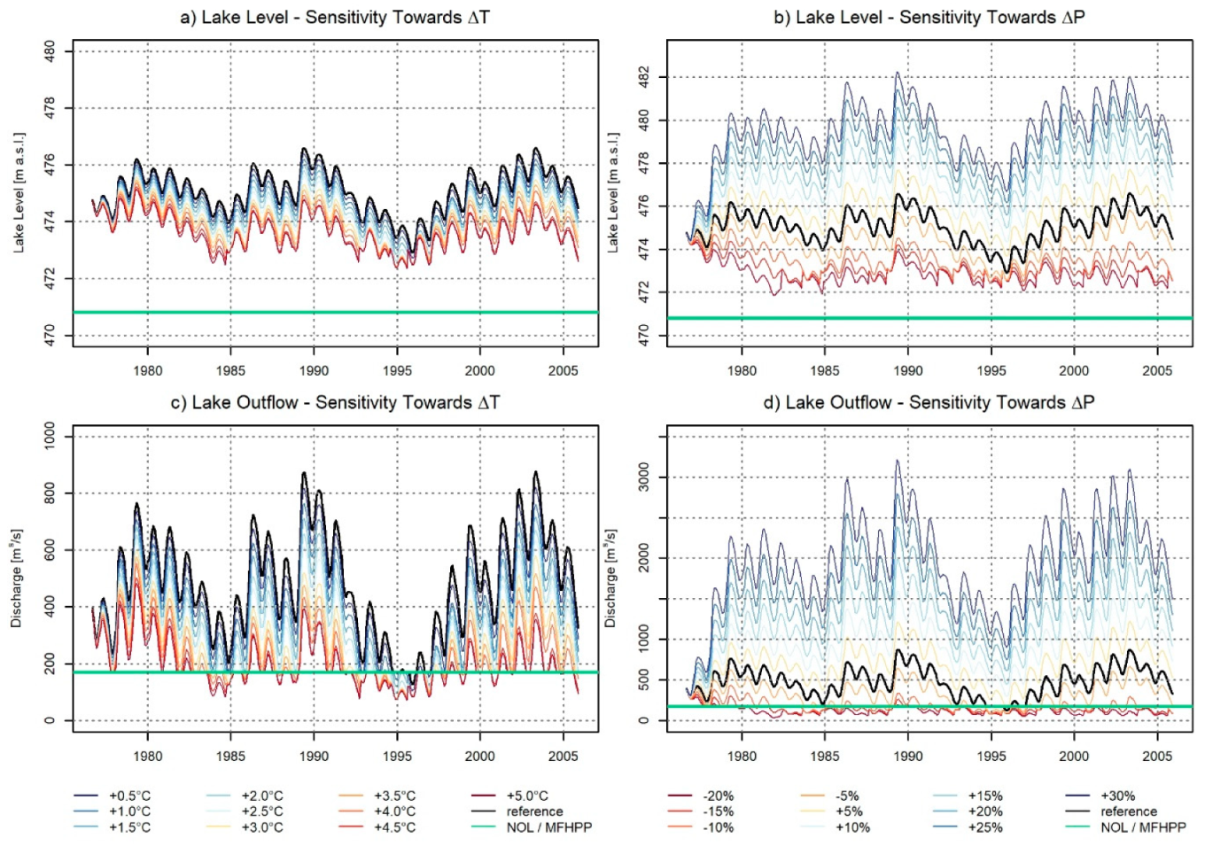
Before applying the hydrological model chain for the investigation of potential climate change impacts, the sensitivity of the reduced model chain towards systemic alterations in precipitation and temperature is tested. Since Lake Malawi is a key component in the hydrological system of the greater Lake Malawi Basin, it is crucial to understand how the lake system reacts to systematic changes in the hydro-meteorological drivers. The effects of systematically changing precipitation, P (at To) and temperature, T (at Po) (as main drivers for catchment evapotranspiration and lake evaporation) input time series from 1976 to 2005 on the simulations of lake level and lake outflow are shown in Figure 6.
Changing precipitation and temperature considerably affect lake levels and corresponding lake outflows. However, the lake level never drops below the No Outflow Level (NOL) of 470.8 m a.s.l., neither by the most extreme change in precipitation (−20%) nor by the most extreme change in temperature (+5 °C) considered here (Figure 6a,b). An increase in temperature of 5 °C reduces the lake level by 1.42 m as compared to the simulations with no modifications in the temperature input data (reference; To, Po). This translates to a decrease rate of about 0.3 m per 1 °C temperature rise. The impacts of changing precipitation input are more pronounced than changing temperature. Here, lake level changes range from −2.28 m (ΔP of −20% in precipitation) to +4.39 m (ΔP of +30% in precipitation). The mean changes in lake level due to precipitation change are larger with increasing precipitation (+0.7 m per +5%) than decreasing precipitation (−0.6 m per −5% change).
Corresponding to changes in lake level, the outflow from Lake Malawi is considerably altered by systematically varying precipitation (at To) and temperature (at Po) inputs. Compared to the reference mean outflow of 481.2 m3/s, as simulated with the original input data sets (reference; To, Po), outflow decreases by 59.8% with a 5 °C temperature increase (52.5% for +4 °C; 43.2% for +3 °C; 30.5% for +2 °C; 17.1% for +1 °C) (Figure 6c). The firm flow of ≥170 m3/s (Maximum Flow For Hydropower Production (MFHPP); green line, Figure 6c) already occurs in less than 5% of the days during the reference period. With increasing temperature, the proportion of days below the MFHPP increases up to 58% for +5 °C (43% for +4 °C; 30% for +3 °C; 19% for +2 °C; 9% for +1 °C).
Changes in mean river flow are even larger with changing precipitation. Precipitation increases of 5% and 30% lead to increases in mean river flow of 47% and 312%, respectively. In turn, river flow decreases by −32% (329.8 m3/s) and −77% (112.5 m3/s), with a decrease in precipitation of 5% and 20%, respectively. The frequency of days below the MFHPP increases by 19% and 93% for a 5% and 20% decrease in precipitation input, respectively. That is, changes in precipitation have a stronger impact on the likelihood of going below the MFHPP than changes in temperature.
It is shown here that an increase in temperature and a decrease in precipitation affect both lake level and lake outflow from Lake Malawi. However, it is also shown that lake outflow never completely ceases with neither a temperature increase of up to 5 °C nor a precipitation decrease down to −20% alone. The effects of combining changes in temperature and precipitation on river flows and corresponding hydropower generation are illustrated in Section 4.4.

4.3. Climate Change Projections for the Greater Lake Malawi Basin

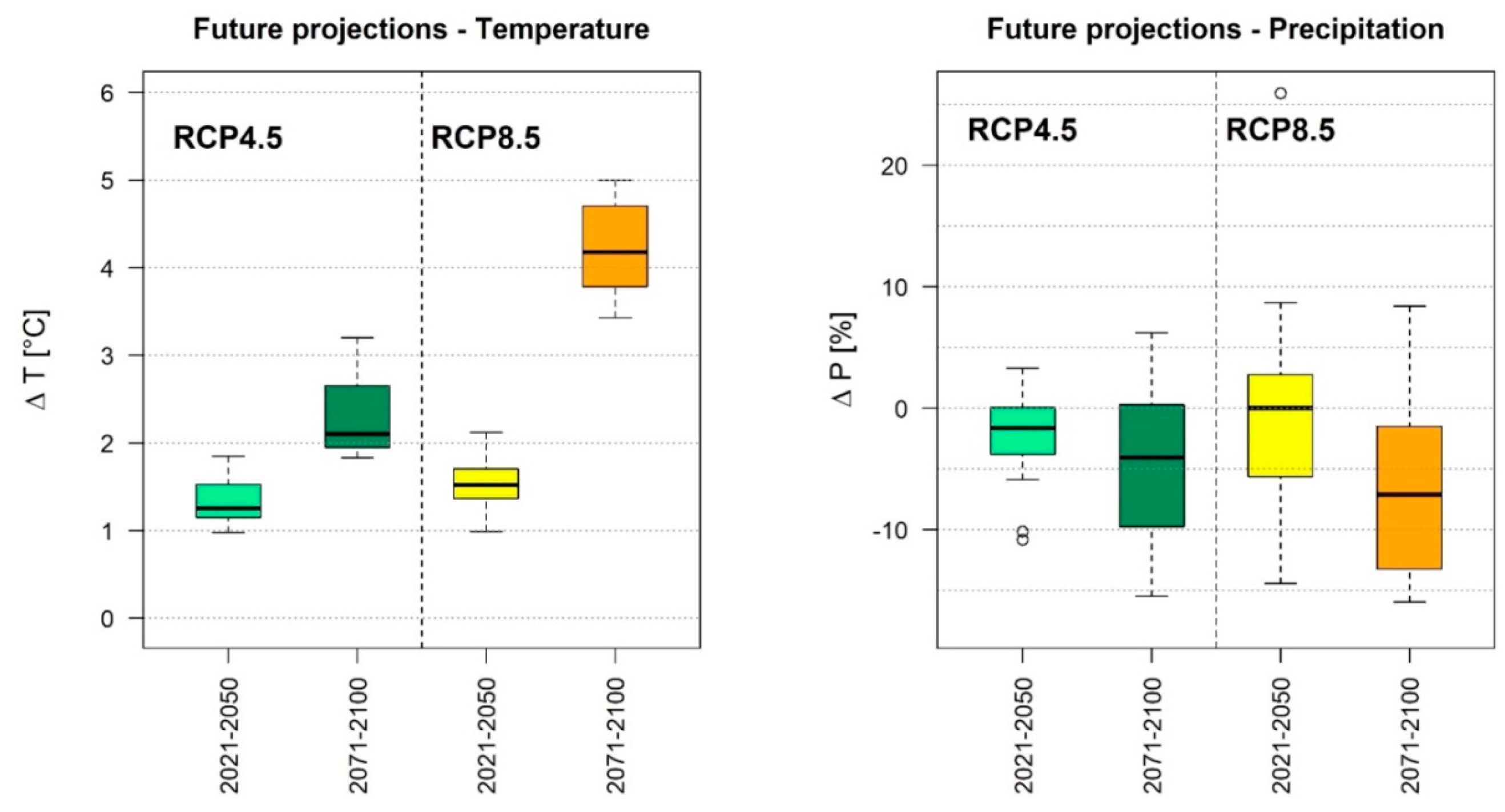
Climate change signals for the near (2021–2050) and far future (2071–2100) scenarios, as they are projected by the considered GCM–RCM combinations (Table 2) from the CORDEX Africa project for the Lake Malawi Basin and Shire River Basin, are summarized in Figure 7. Change signals refer to the reference period 1976 to 2005.
For the near future period, the ensemble projections indicate an average increase in temperature of 1.32 °C (range: 0.98, 1.85) and 1.55 °C (0.99, 2.12) for the RCP4.5 and RCP8.5, respectively. For the far future period, the ensemble projections indicate an average increase in temperature of 2.3 °C (1.8, 3.2) and 4.2 °C (3.4, 5.0) for the RCP4.5 and RCP8.5, respectively. The spread of the ensemble projections, which indicates the ensemble uncertainty, is considerably larger for the far future period than for the near future period irrespective of the concentration pathway considered.
Projections for changes in precipitation are not as definite as for temperature, although the ensemble mean for all considered periods and concentration pathways indicate a decrease in future precipitation. For the near future period, the ensemble projections indicate an average decrease in precipitation of −2.2% (range: −11, +3) and −0.63% (−14, +26 (outlier); +9 (upper whisker)) for the RCP4.5 and RCP8.5, respectively. For the far future period, the ensemble projections indicate an average precipitation decrease of −4.6% (−15, +6) and −7.1% (−16, +3) for the RCP4.5 and RCP8.5, respectively. As indicated by the range of the projections, the ensemble of GCM–RCM combinations does not entirely agree on the direction of change: at least one model (far future; RCP8.5) and a maximum of nine model (near future; RCP8.5) projections indicate an increase in precipitation rather than a decrease, while four and five models for RCP4.5 (near) and RCP4.5 (far), respectively, indicate a positive increase. The uncertainty is larger for RCP8.5 than RCP4.5 for the near future. In general, the spread of the ensemble is larger for precipitation than for temperature.

4.4. Climate Change Impacts on Water Budgets and Hydropower Productivity

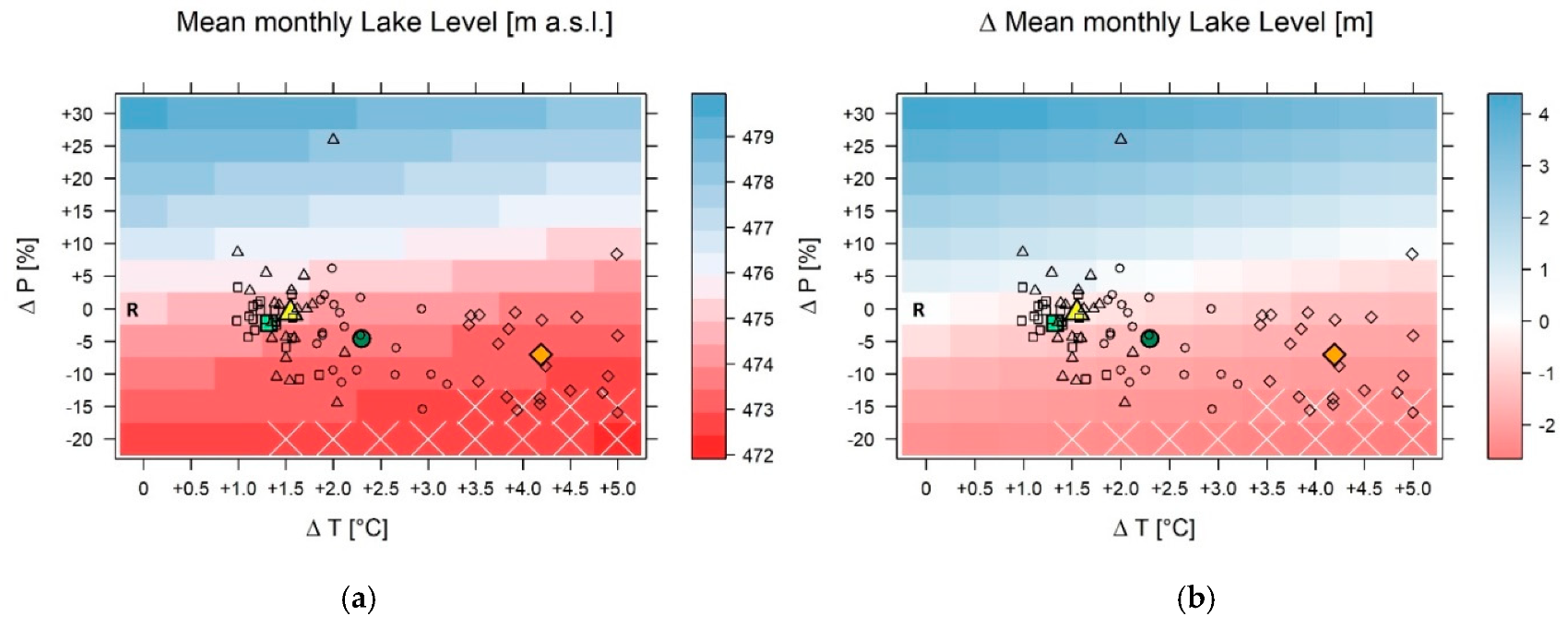
Here, we combine the insights of the sensitivity analysis (c.f. Section 4.2) with the projected changes in temperature and precipitation (c.f. Section 4.3) to investigate the potential impacts of climate change on lake level, Shire River discharge and corresponding hydropower productivity and reliability by means of response surfaces. Each pixel in the response surface indicates the simulated impact (color coded) of a certain combination of changes in mean annual temperature and precipitation (ΔT, x-axis; ΔP, y-axis) on the specific target variable. The reference pixel (i.e., no change in hydro-climatological conditions; ΔT = 0, ΔP = 0) is marked by an “R”. Overlaid, colored symbols illustrate the mean climate change signal from the CORDEX Africa ensemble projections for both periods and RCPs considered (same colors as in Figure 7). The corresponding hollow symbols refer to the climate change signals from the individual ensemble members and illustrate the ensemble range (i.e., the uncertainties in the projections). That is, the reader can easily assess likely future changes (impacts) as projected by the climate models within the domain of the response surface.

4.4.1. Lake Level

Figure 8 shows the response surfaces for absolute and relative changes in lake level as simulated by the ULMBM and the LMM using all the combinations of perturbed meteorological input data. The figure shows the relative changes with reference to the simulated mean lake level based on observed temperature (To) and precipitation (Po) (R-labeled pixel in Figure 8) for the period 1976–2005.
The response surfaces demonstrate that the estimates for mean lake level range between 472.4 (ΔT +5 °C; ΔP −20%) and 479.4 m a.s.l. (ΔT 0 °C; ΔP +30%) (Figure 8a) which refers to relative changes of −2.6 m and +4.4 m (Figure 8b) compared to the reference mean (ΔT 0 °C and ΔP 0%) lake level of 475 m a.s.l. (1976–2005). Both decreasing annual precipitation and increasing temperature lead to a decrease in the mean water levels of Lake Malawi. The influence of scaling precipitation on lake level changes is slightly larger than scaling temperature, although temperature scaling alone already accounts for a decrease in mean lake level of 1.4 m (ΔT +5 °C; ΔP 0%)). For the combinations of scaling precipitation and temperature by ΔP −15% (−20%) and ΔT 3.5 °C (1.5 °C), the simulations indicate that lake level decreases to an extent so that the level is temporally below 470.8 m a.s.l. (crossed pixels in Figure 8) during some days of the year and this leads to a temporal absence of outflow from Lake Malawi into the Shire River. It is noteworthy that this situation does not occur when only one parameter is scaled, as shown by the sensitivity analysis (cf. Section 4.2 and Figure 6).
The ensemble means of the climate projections (colored symbols) indicate that the mean lake level in the near future period (2021–2050) is projected to decrease by/to 1.1 m/473.9 m a.s.l. (RCP4.5) and 0.5 m/474.5 m a.s.l. (RCP8.5). In the far future period (2071–2100), lake level is projected to decrease by/to 1.5 m/473.5 m a.s.l. (RCP4.5) and 2.1 m/472.9 m a.s.l. (RCP8.5) (summary in Table 3). The spread of the models (different symbols), though, is rather large and some individual climate models even suggest an increase in lake level for some periods and scenarios considered. However, seven GCM–RCM combinations for the far future period and RCP8.5 indicate changes in mean annual temperature and precipitation sums, which will lead to a temporal absence of outflow from Lake Malawi.

4.4.2. Shire River Discharge at Liwonde

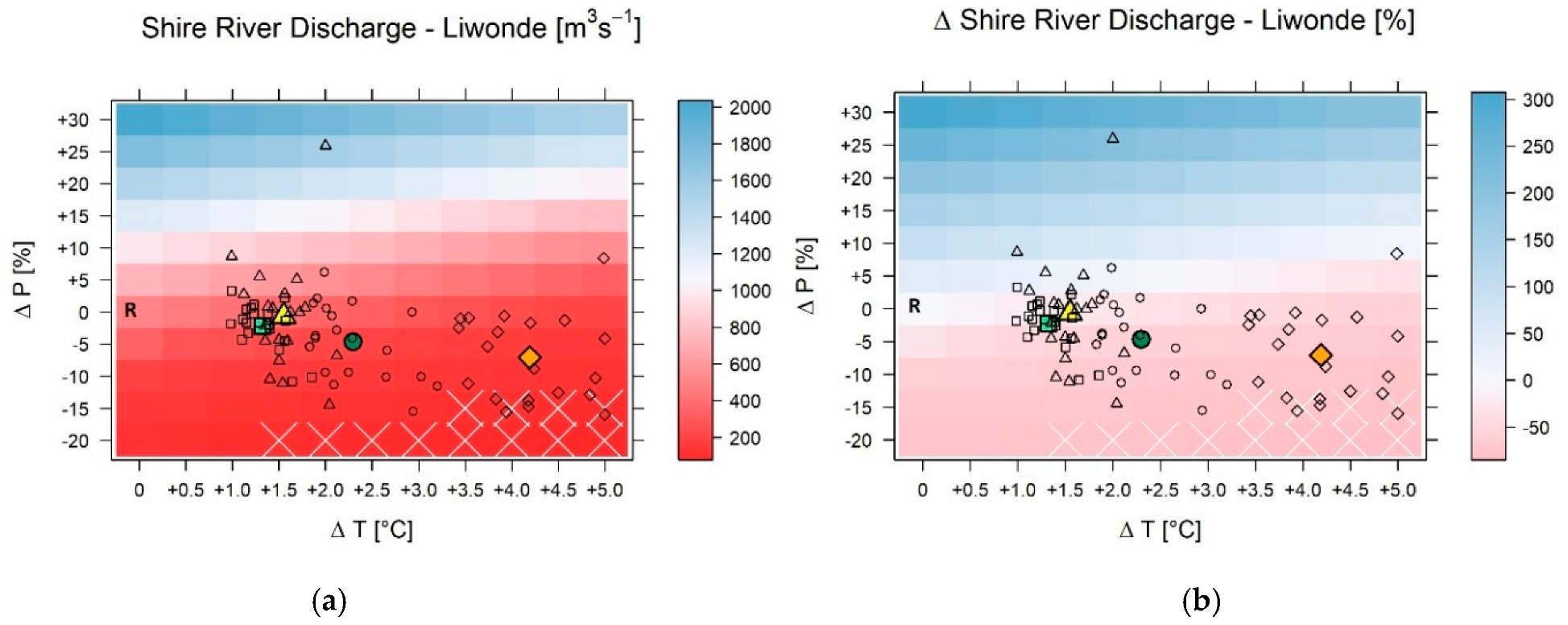
Figure 9 presents response surfaces illustrating the absolute and relative changes in Shire River discharge at the Liwonde gauge derived by the entire hydrological model chain using systematically perturbed meteorological observations as input.
In terms of absolute river discharge, Figure 9a demonstrates that the mean annual discharge at Liwonde ranges from ~75 m3/s (ΔT +5 °C; ΔP −20%) to ~2000 m3/s (ΔT 0 °C; ΔP +30%). This refers to relative changes of −84% to +307%, respectively (Figure 9b). With increasing temperature (as a proxy for increasing evapotranspiration) and decreasing precipitation sums, river discharge in the Shire River decreases. As expected, the lowest discharge values are found for the combinations of lowest precipitation and highest temperature changes, while the largest discharge values are found for the opposite combination. Changes in river discharge are predominantly driven by scaling precipitation, although temperature also impacts the changes in discharge since the color changes in the plots (Figure 9) are not strictly horizontal but slightly diagonal. The effect of temperature scaling, however, is not as distinctive as for lake level changes (see Figure 8). As indicated by the mean of the climate projection ensembles (colored symbols, Figure 9), the reference (current) mean discharge of ~500 m3/s will likely decrease by/to −49%/253 m3/s (RCP4.5) and −23%/385 m3/s (RCP8.5) in the near future period, and by/to −59%/202 m3/s (RCP4.5) and −75%/127 m3/s (RCP8.5) in the far future period (Table 3). The large spread of the ensemble members, though, indicates that some individual cases project an increase in Shire River discharge. However, most of the ensemble members for every period and scenario considered indicate a decrease in discharge between −50% and −76% (interquartile range; i.e., 25%–75% of the ensemble distribution).

4.4.3. Hydropower Productivity

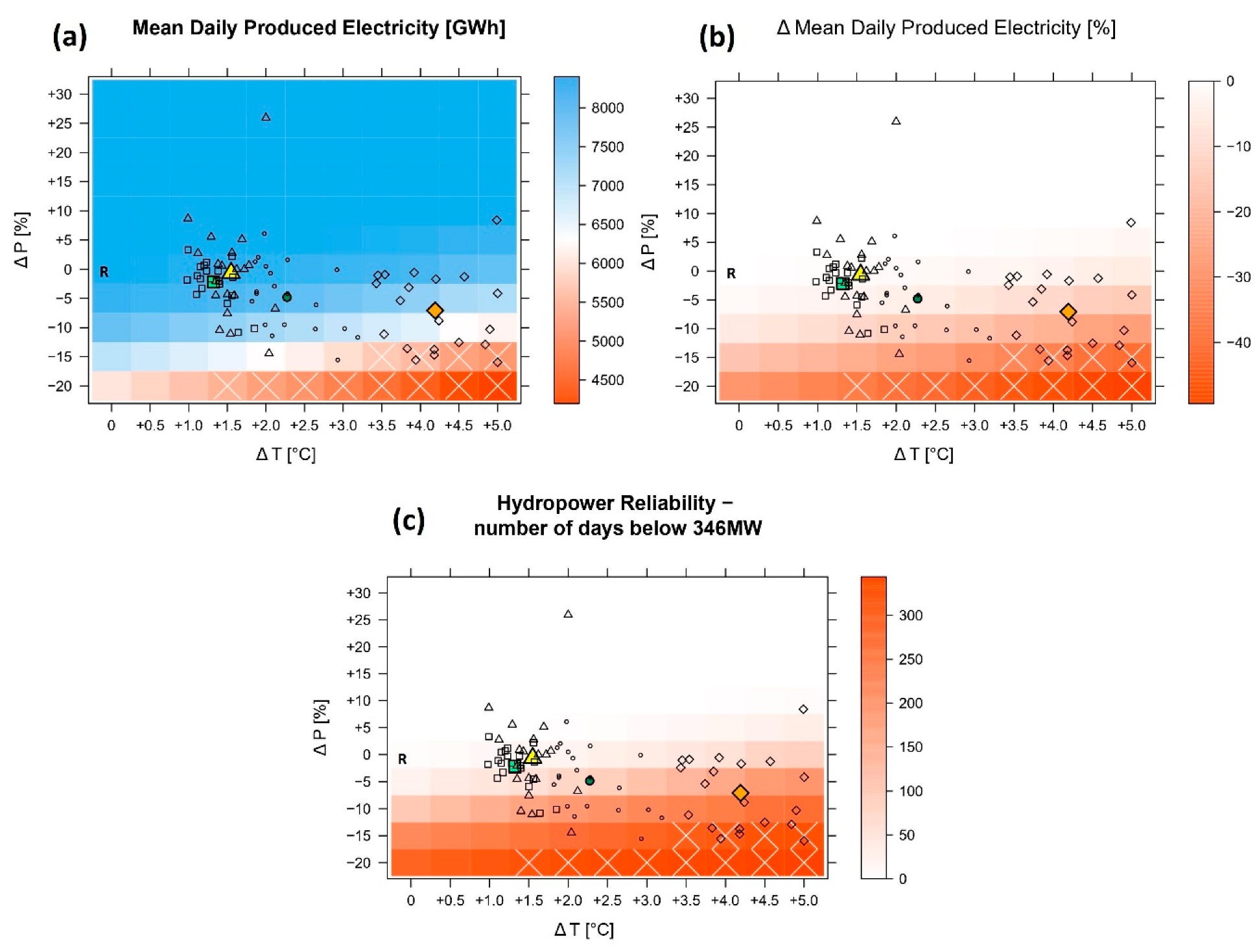
Figure 10 presents the response surfaces illustrating absolute (a; in GWh) and relative changes (b; in % differences from reference mean) in agglomerated mean hydropower production in the middle Shire River (in terms of mean daily produced electricity). Hydropower production is estimated based on discharge simulations derived by the hydrological model chain driven with systematically perturbed meteorological observation data as input. Hydropower reliability (Figure 10c) indicates the number of days with hydropower productivity below 346.3 MW (maximum production) per year.
As long as the river discharge is above the MFHPP threshold (see Figure 6c,d), the installed maximum daily hydropower production is 8310 GWh. That is, with the currently installed hydropower infrastructure, no more hydropower can be produced even if the discharge in the Shire River increases. However, the mean daily hydropower production (as simulated by the hydrological model chain) for the reference period (To and Po) is 8304 GWh, indicating that the impacts of climate on hydropower production are already manifesting themselves. However, when the precipitation increases by 5%, the maximum production is realized as long as the temperature increase remains less than 2 °C (thus ΔP ≥ +5%; ΔT ≤ 2 °C) or when the precipitation increases by 10% and the temperature increase is below 5 °C (thus ΔP ≥ +10%; ΔT ≤ 5 °C). This situation makes the number of days without maximum electricity production, which is currently at 4 days (To and Po), reduce to zero days (Figure 10c). For all the other combinations of changes in temperature and precipitation, hydropower productivity decreases up to 4206 GWh (ΔT +5 °C; ΔP −20%) which is a reduction of −49%. This results in a considerable decline in hydropower reliability: 344 days per year when the daily maximum electricity production of 346.3 MW is not reached. The mean of the ensemble climate projections (colored symbols) consistently indicates a decrease in hydropower productivity and reliability for all the periods and scenarios considered. For the near future period, the decrease in mean production is by/to −2.5%/8046 GWh (RCP4.5) and −0.7%/8244 GWh (RCP8.5). This corresponds to 46 (RCP4.5) and 16 days (RCP8.5) without maximum electricity production per year (Table 3). For the far future period, the decrease in production indicated by the ensemble climate mean projections is about −5%/7879 GWh (RCP4.5) and −24%/6291 GWh (RCP8.5). This corresponds to 89 and 259 days without maximum hydropower production (Table 3). Again, we need to emphasize the marked uncertainty in this regard, i.e., the spread of the models includes individual model projections which suggest no decrease in hydropower productivity and reliability and several projections which indicate a decrease much larger than those suggested by the ensemble means. For instance, seven GCM–RCM combinations for the far future period and RCP8.5 indicate a decrease in hydropower productivity between 33 and 38% (5535 GWh and 5138 GWh) and a corresponding hydropower reliability between 300–318 days (production below currently installed capacity).

5. Discussion

5.1. Sensitivity of Water Resources to Changes in Precipitation and Temperature (Evapotranspiration)

Our analyses have shown that lake level and outflow are highly sensitive to changes in precipitation and temperature. As expected, the influence of changing precipitation on lake level and outflow is stronger than the influence of changing temperature. However, the decrease of 0.3 m in lake level and 17% in lake outflow per 1 °C temperature increase clearly demonstrates the important role of evapotranspiration in the hydrological system of the Lake Malawi Basin. The effects of evapotranspiration are also detected in the Shire River discharge and corresponding hydropower productivity. They are, however, not as large as for the hydrological parameters of the lake system. The effects of altered evapotranspiration on the Shire River can rather be seen as a translation of such effects on lake outflow downstream to the Shire River. This underlines the particular role of (changing) lake evaporation, including its relevance to lake outflow, which is substantial for water supply and energy production on the Shire River. Note, however, that these statements are based on changing temperature as a single driver for altered evapotranspiration. The detection of actual changes in evapotranspiration would require more detailed, physically based analyses which should also consider changes in radiation budget, e.g., through altered cloud cover and/or the feedback effect of air humidity, for instance, which may amplify or dampen the effects. Still, the increasing relevance of lake evaporation due to increasing temperature agrees with findings in other regions such as Lake Victoria [75,76].
As shown by the response surface generated in this study, the combination of decreasing precipitation and increasing temperature would lead to even more severe impacts on lake level, outflow, river discharge and energy production. Here, we found that 12 out of 121 hydrological model simulations project temporally ceasing outflow from Lake Malawi into the Shire River, which will transform the upper Shire River from a perennial to a seasonal river. As we have shown that temporally ceasing outflow may already occur for temperature increases from +1.5 °C, this highlights the importance of the global warming limit of 1.5 °C, as agreed by the United Nations Framework Convention on Climate Change (UNFCCC) in 2015 [77]. The transformation of the Shire River to a seasonal river would have serious consequences on fresh water supply, irrigation, river ecology and hydropower generation further downstream. For 2071–2100, seven out of 20 climate projections suggest such a situation, which highlights that there is a real risk of such a scenario. Here, we refer to Bhave et al. [31], who detected in 11 out of 30 climate projections with a seasonal instead of perennial outflow from Lake Malawi from 2020 to 2050. However, they used bias-corrected CMIP5 GCM projections and not CORDEX Africa data, and they considered the no outflow threshold for lake level to be 471.5 m a.s.l.; i.e., 0.6 m higher than the threshold suggested by Kumambala and Ervine [25], which is used in this study. Moreover, Bhave et al. [31] investigated the risk of lake level going below the no outflow threshold primarily by changes in precipitation (and land evapotranspiration) assuming constant lake evaporation [31]. Given the sensitivity of the hydrological system towards changes in lake evaporation as sketched out by our study, the risk of temporally ceasing lake outflow is presumably even larger than reported by Bhave et al. [31] based on their model setup. Another remarkable difference from the study of Bhave et al. [31] is that we could identify only very few scenarios which may lead to an increase in mean lake level, while Bhave et al. [31] identified nine out 30 climate models leading to such a situation. This generally highlights the sensitivity of climate change impact studies towards the choices made during the setup of model chains.

5.2. Climate Change Impacts on Hydropower Productivity

The mean ensemble projections of temperature and precipitation changes for 2021–2050 and 2071–2100 indicate gradually increasing temperature and decreasing precipitation for both scenarios considered. These combinations lead to a considerable decrease in Shire River discharge, and thus also in hydropower productivity. The hydropower production is under threat due to these changes, with a reduction between −1% and −24% depending on the period and scenario. That is, the critical flow of 170 m3/s, which is required for a maximum utilization of the installed hydropower capacity, is sometimes not met by all ensemble means considered in this study. Extreme scenarios even suggest a reduction in hydropower productivity up to 38%, with 318 days per year without maximum production, which coincides with a temporal lack of outflow from Lake Malawi. This will seriously endanger the reliability of electricity supply in Malawi and even risk more occasional power blackouts in the country.
The differences between the RCP4.5 and RCP8.5 scenarios and the spread of the individual ensembles (i.e., the uncertainties in the climate projections) are large. Still, water management and hydropower companies need to include likely variations in river discharge due to climate change in their future planning, e.g., by expanding hydropower capacity to meet current and future demands, or by introducing annual and diurnal optimization of electricity production responding to demand variations. Already, power deficits occur occasionally [78,79] and our simulation indicates that the present hydropower reliability is at 4 days per year (4 days when maximum hydropower production is not reached). Therefore, decreasing hydropower production will have large implication for the economy in Malawi since energy is the main driver for economic development. Already, recent power supply deficits have had negative impacts on the economy and development. Referring to Brailovskaya [78], about 25% of daily business profits are lost due to power outages, and the country loses more than 6% of its annual GDP due to these power cuts [79]. Therefore, future plans for hydropower development need to incorporate measures for sustaining electricity production in times of climate change.
Around the globe, there are a number of watersheds where related conditions or problems are similar, e.g., where uncertainty in future hydropower productivity may increase due to changes in climate. For example, such conditions are also projected in some regions of Brazil, such as the Sao Francisco basin in central Brazil [80] or in the Amazon region [81]. In the latter, the problems are exacerbated by ongoing heavy deforestation [81]. However, the case of Malawi is particularly interesting (and possibly vulnerable) because the ratio between lake surface area and the surrounding catchment area is rather large, probably among the largest in the world. This is why open water (i.e., lake surface) evaporation is important in this case and makes this coupled hydro-system rather unique.

5.3. Limitations and Uncertainties

This study faces several limitations and uncertainties, which request some assumptions in the study design and need to be taken into account when evaluating the results. First, there are some constraints regarding the hydro-meteorological observation data for the Lake Malawi and Shire River basins in terms of spatial and temporal data coverage. As illustrated in Section 2.2, we needed to take into account the gridded GPCC data sets for the Tanzanian and the Mozambican parts of the Lake Malawi Basin due to the unavailability of meteorological station data. In addition, inflow into Lake Malawi is rarely gauged at the tributaries of the lake. Gauge Zayuka on the Luweya River, which we used for the calibration of the ULMBM, provides the best data quality in terms of reliability and temporal coverage. Still, it is hardly possible to calibrate and verify the ULMBM at gauges in other tributaries. This limits the confidence in the hydrological model to simulate all aspects of lake inflow sufficiently well at intra-annual timescales. The estimation of lake evaporation as a key process within the lake model is prone to notable uncertainties because of limited data to assess energy budgets. For instance, we used maximum and minimum temperature to estimate net radiation. Moreover, evaporation estimates cannot be verified against observation data due to the unavailability of direct measurements of evaporation from the lake surface. However, the calibration and verification of all the three components of the hydrological model chain show good matches with available observations, which underline the suitability of the proposed approach for our study purpose.
In our model setup, we implement the operation guidelines for the barrage at Liwonde, which controls lake outflow and discharge in the upper Shire River. Observation data, though, indicate that these operation rules are often violated, presumably to allow for sufficient river discharge in the Shire River during severe drought situations (e.g., in the 1990s). This limits the time periods which can be used for the calibration and verification of the SRM. For the future scenarios in this study, we assume the operation guidelines to be active as proposed, although it is likely that barrage operation will adapt to lower lake levels in the future [31].
The response surfaces are generated using the simplest way of perturbing the meteorological input data, which does not account for possible changes in the temporal sequencing of climate input data (i.e., the annual, seasonal and day-to-day variability). This criticism is similar to the disadvantage of using delta change approaches for statistically downscaling climate model data [72]. Several alternative response surface approaches are published that (partly) take changes in temporal sequencing into account [1,66]. However, since we are interested in changes in long-term mean values of the water budget, the issue of changes in the temporal sequencing of the meteorological input data is considered less important, as suggested by Bronstert et al. [82].
This study investigates the potential impacts of changes in climate conditions and does not consider changes in land use and land cover or water abstraction for irrigation. However, changes in land cover and expansion in irrigation farming in the course of the socio-economic development in Malawi, as has happened in the recent past can be expected to continue/expand in the future, that will also influence the hydrological system of the basin [37,38,39].
Lastly, the estimation of changes in the hydrological system of the basin are based on only one hydrological model using one best fit model parameter set for each component within the model chain. To explore the uncertainty of the hydrological projections in more detail, a more comprehensive model setup including more model structures and parameter sets would be necessary.

6. Conclusions

In this study, we assessed the sensitivity of the hydrological system of the Lake Malawi and Shire River basins to estimate potential impacts of future climate on key hydrologic variables and on hydropower generation on the Shire River. We have adapted the mesoscale Hydrological Model (mHM) to the catchments of the Lake Malawi and Shire River basins. A lake model was developed and linked between the hydrological models of the upper Lake Malawi Basin (ULMBM) and the Shire River Basin (SRM). This lake model accounts for reservoir attenuation effects and dynamic lake water balances, such as rainfall on the lake, inflow from the upper Lake Malawi catchment and evaporation losses, yielding lake level and lake outflow dynamics. This calibrated and verified hydrological model chain was used to estimate the sensitivity of water levels of Lake Malawi and the corresponding discharge and hydropower production on the Shire River to systematic changes in temperature and precipitation by means of response surfaces. Reconsidering the three guiding research questions of this study, we can draw the following conclusions:
  • The role of lake evaporation is essential for changes in lake level and lake outflow. Note that, currently, lake evaporation clearly exceeds rainfall over the lake. Although the effects of projected future rainfall changes on lake level and outflow were slightly larger than the effects of temperature changes, the sensitivity analysis identified the particular role of lake evaporation for the hydrological system of Lake Malawi. Evapotranspiration effects (temperature increases as a proxy) on Shire River discharge are not as high as for the lake surface area, and they might be seen as the inherited influence of outflow sensitivity from the lake.
  • Climate projections agree that gradually increasing temperature and decreasing precipitation lead to a reduction in mean lake level, outflow and Shire River discharge. Depending on the time period and scenario considered, mean lake level and Shire River discharge are projected to decrease in in range of 0.5 m to 2.1 m and 23% to 75%, respectively. However, extreme scenarios even suggest a decrease in lake level, which would lead to a temporally ceasing outflow from Lake Malawi into the Shire River, bringing along serious ecological and economic threats. These results demonstrate that this tropical hydro-system is particularly vulnerable to climate change impacts. Since water resources are crucial for the economic development of Malawi, this may have serious socio-economic consequences for the country.
  • Based on the currently installed capacities, hydropower productivity and reliability decrease for all future scenarios considered. The degree of these decreases, however, strongly depends on the time periods and scenarios considered. On average, projections for hydropower production losses vary between −1% and −24% (thus for 16 to 259 days per year, the maximum electricity production will not be reached). In part, the adverse effects of reduced Shire discharge on electrical production can be counteracted by installing additional hydropower stations along the middle Shire and/or the seasonal and diurnal optimization of hydro-electric production. This strategy is currently followed in Malawi, as some new power stations are under construction or planned [18,19,20]. Still, extreme scenarios, which coincide with a temporal offset of outflow from Lake Malawi, even suggest a productivity loss by −38%, with 318 days per year without maximum production. This would seriously endanger the domestic energy supply in Malawi.
For all climate change projections, though, we need to emphasize that the uncertainties are large. Still, decision makers need to be cautious and develop reasonable adaptation strategies to secure future water and energy demands based on the detected possible outcomes highlighted in this study.

Author Contributions

Conceptualization: L.M., K.V., A.B.; Methodology, L.M., A.B. and K.V.; formal analysis, L.M. and K.V.; visualization, L.M. and K.V.; supervision, A.B., K.V.; writing original draft, L.M.; editing and reviewing, K.V., A.B., P.K. and P.S.; software, P.S., K.V.; data curation, P.K. All authors have read and agreed to the published version of the manuscript.

Funding

This work was supported by the part-time scholarship of the Potsdam Graduate School at the University of Potsdam (UP), additional funds have been received from the Research and Training School “Natural Hazards and Risks in a Changing World (NatRiskChange)” at UP funded by the German Research Foundation (DFG).

Acknowledgments

We wish to thank the Department of Water Resources and Climate Change and Meteorological Services in Malawi for river discharge, lake level and rainfall data support. We would also like to thank the Helmholtz Centre for Environmental Research (UFZ), in particular Luis Samaniego, Oldrich Rakovec and Sabine Attinger for mHM support. We also acknowledge the support rendered by Elena McDonnel and Martin Schuttig during the development of the lake model.

Conflicts of Interest

The authors declare no conflict of interest.

References

  1. Vormoor, K.; Rössler, O.; Bürger, G.; Bronstert, A.; Weingartner, R. When timing matters-considering changing temporal structures in runoff response surfaces. Clim. Chang. 2017, 142, 213–226. [Google Scholar] [CrossRef]
  2. Bates, B.C.; Kundzewicz, Z.W.; Wu, S.; Palutikof, J.P. Climate Change and Water. Technical Paper of the Intergovernmental Panel on Climate Change; IPCC: Geneva, Switzerland, 2008; Volume 100. [Google Scholar]
  3. Shukla, P.R.; Skea, J.; Slade, R.; Diemen, E.; Haughey, E.; Malley, J.; Pathak, J.; Pereira, P. Climate Change and Land an IPCC Special Report on Climate Change, Desertification, Land Degradation, Sustainable Land Management, Food Security, and Greenhouse Gas Fluxes in Terrestrial Ecosystems; Shukla, P.R., Skea, J., Slade, R., Diemen, R., Haughey, E., Malley, J., Pathak, M., Pereira, J.P., Eds.; IPCC: Geneva, Switzerland, 2019. [Google Scholar]
  4. Simms, A. Africa: Up in Smoke?: Second Report from the Working Group on Climate Change and Development; Murphy, M., Ed.; The New Economics FoundationOxfam GB: London, UK, 2006; pp. 4–44. [Google Scholar]
  5. Luo, T.; Young, R.; Reig, P. Aqueduct Projected Water Stress Country Rankings; Technical Note; World Resources Institute: Washington, DC, USA, 2015. [Google Scholar]
  6. Arnell, N.W. Climate change and global water resources: SRES emissions and socio-economic scenarios. Glob. Environ. Chang. 2004, 14, 31–52. [Google Scholar] [CrossRef]
  7. IPCC. Summary for Policymakers. In Climate Change 2007: The Physical Science Basis; Solomon, S., Qin, D., Manning, M., Chen, Z., Marquis, M., Averyt, K.B., Tignor, M., Miller, H.L., Eds.; Cambridge University Press: Cambridge, UK, 2007. [Google Scholar]
  8. Kusangaya, S.; Warburton, M.L.; Archer van Garderen, E.; Jewitt, G.P.W. Impacts of climate change on water resources in southern Africa: A review. Phys. Chem. Earth 2014, 67–69, 47–54. [Google Scholar] [CrossRef]
  9. Taulo, J.L.; Gondwe, K.J.; Sebitosi, A. Ben Energy supply in Malawi: Options and issues. J. Energy South. Africa 2015, 26, 19–32. [Google Scholar] [CrossRef] [Green Version]
  10. ESCOM. The Effect of the Current Rainfall on Water Levels and Electricity Supply (Generation). Available online: http://www.escom.mw/rainfall-effect-waterlevels.php (accessed on 22 March 2017).
  11. Shela, O.N. Naturalisation of Lake Malawi levels and Shire River flows. In Proceedings of the 1st WARFSA/WaterNet Symposium: Sustainable Use of Water Resources, Maputo, Mozambique, 1–2 November 2000; pp. 1–2. [Google Scholar]
  12. Mtilatila, L.; Bronstert, A.; Bürger, G.; Vormoor, K. Meteorological and hydrological drought assessment in Lake Malawi and Shire River Basins (1970–2013). Hydrol. Sci. J. accepted for publication.
  13. Beck, L.; Bernauer, T. How will combined changes in water demand and climate affect water availability in the Zambezi river basin? Glob. Environ. Chang. 2011, 21, 1061–1072. [Google Scholar] [CrossRef]
  14. Mujere, N.; Mazvimavi, D. Impact of climate change on reservoir reliability. Afr. Crop Sci. 2012, 20, 545–551. [Google Scholar] [CrossRef]
  15. Stevens, T.; Madani, K. Future climate impacts on maize farming and food security in Malawi. Sci. Rep. 2016, 6, 36241. [Google Scholar] [CrossRef] [Green Version]
  16. Tadross, M.; Jack, C.; Hewitson, B. On RCM-based projections of change in southern African summer climate. Geophys. Res. Lett. 2005, 32, 1–4. [Google Scholar] [CrossRef]
  17. Arnell, N.W.; Hudson, D.A.; Jones, R.G. Climate change scenarios from a regional climate model: Estimating change in runoff in southern Africa. J. Geophys. Res. D Atmos. 2003, 108. [Google Scholar] [CrossRef]
  18. Yanda, P. Climate Change, Adaptation and Higher Education-Securing our Future. In SARUA Leadership Dialogue Series Volume 2 Number 4; Kotecha, P., Ed.; SARUA: Cape Town, South Africa, 2010. [Google Scholar]
  19. Conway, D.; Curran, P.G.K.E. Policy Brief: Climate Risks to Hydro-Power Supply in Easte rn and Southern Africa; Grantham Research Institute on Climate Change and Environment: London, UK, 2018. [Google Scholar]
  20. GOM. Malawi Electricity Investment Plan; Department of Energy Affairs: Lilongwe, Malawi, 2010. [Google Scholar]
  21. Milleniun Challenge Corporation. Investment Outlook-Business Opportunities in Malawi Power Sector. Lilongwe, Malawi, 2015. Available online: https://www.mcc.gov/resources/pub-full/star-report-malawi (accessed on 7 August 2020).
  22. Harrison, G.P.; Whittington, H.W. Susceptibility of the Batoka Gorge hydroelectric scheme to climate change. J. Hydrol. 2002, 264, 230–241. [Google Scholar] [CrossRef] [Green Version]
  23. Kaunda, C.S.; Mtalo, F. Impacts of environmenta degradation and climate change on electricity generation in Malawi. Int. J. Energy Environ. 2013, 4, 1101–1112. [Google Scholar]
  24. Gosling, S.N.; Arnell, N.W. A global assessment of the impact of climate change on water scarcity. Clim. Chang. 2016, 134, 371–385. [Google Scholar] [CrossRef] [Green Version]
  25. Kumambala, P.G.; Ervine, A. Water Balance Model of Lake Malawi and its Sensitivity to Climate Change. Open Hydrol. J. 2010, 4, 152–162. [Google Scholar] [CrossRef] [Green Version]
  26. Mazvimavi, D. Climate change, water availability and supply. In Climate Change, Adaptation and Higher Education: Securing Our Future; Kotecha, P., Ed.; SARUA: Cape Town, South Africa, 2010. [Google Scholar]
  27. Ngigi, S.N. Climate Change Adaptation Strategies: Water Resources Options for Smallholder Farming Systems in Sub-Saharan Africa; The Earth Institute at Columbia University: New York, NY, USA, 2012. [Google Scholar]
  28. Makungwa, S. Adaptation, Agrivulture and Food Security. In Climate Change, Adaptation and Higher Education: Securing our Future; Kotecha, P., Ed.; SARUA: Cape Town, South Africa, 2010. [Google Scholar]
  29. Saka, J.D.K.; Sibale, P.; Hachigonta, S.; Sibanda, L.M.; Thomas, T.S. Southern African Agriculture and Climate Change: A Comprehensive Analysis-Malawi; International Food Policy Research: Washington, DC, USA, 2012. [Google Scholar]
  30. Lotz-Sisitka, H. Knowledge Questions Associated with the Public Health and Climate Change Relation: Some Implications for Universities in Southern Africa. In Climate Change, Adaptation and Higher Education: Securing Our Future; Kotecha, P., Ed.; SARUA: Cape Town, South Africa, 2010. [Google Scholar]
  31. Bhave, A.G.; Bulcock, L.; Dessai, S.; Conway, D.; Jewitt, G.; Dougill, A.J.; Kolusu, S.R.; Mkwambisi, D. Lake Malawi’s threshold behaviour: A stakeholder-informed model to simulate sensitivity to climate change. J. Hydrol. 2020, 584, 124671. [Google Scholar] [CrossRef]
  32. Arndt, C.; Schlosser, A.; Strzepek, K.; Thurlow, J. Climate change and economic growth prospects for Malawi: An uncertainty approach. J. Afr. Econ. 2014, 23, 83–107. [Google Scholar] [CrossRef] [Green Version]
  33. Yamba, F.D.; Walimwipi, H.; Jain, S.; Zhou, P.; Cuamba, B.; Mzezewa, C. Climate change/variability implications on hydroelectricity generation in the Zambezi River Basin. Mitig. Adapt. Strateg. Glob. Chang. 2011, 16, 617–628. [Google Scholar] [CrossRef] [Green Version]
  34. Kachaje, O.; Kasulo, V.; Chavula, G. The potential impacts of climate change on hydropower: An assessment of Lujeri micro hydropower scheme, Malawi. Afr. J. Environ. Sci. Technol. 2016, 10, 476–484. [Google Scholar] [CrossRef] [Green Version]
  35. Munthali, G.; Saka, J.; Kamdonyo, D.; Kasulo, V.; Nkhokwe, J.; Kainja, S. Drought Case Study for Malawi; Department of Meteorological Services: Blantyre, Malawi, 2003. [Google Scholar]
  36. Jury, M.R.; Mwafulirwa, N.D. Climate variability in Malawi, Part 1: Dry summers, statistical associations and predictability. Int. J. Climatol. 2002, 22, 1289–1302. [Google Scholar] [CrossRef]
  37. Chavula, G.; Brezonik, P.; Bauer, M. Land Use and Land Cover Change (LULC) in the Lake Malawi Drainage Basin, 1982–2005. Int. J. Geosci. 2011, 2, 172–178. [Google Scholar] [CrossRef] [Green Version]
  38. Palamuleni, L.G.; Ndomba, P.M.; Annegarn, H.J. Evaluating land cover change and its impact on hydrological regime in Upper Shire river catchment, Malawi. Reg. Environ. Chang. 2011, 11, 845–855. [Google Scholar] [CrossRef]
  39. Calder, I.R.; Hall, R.L.; Bastable, H.G.; Gunston, H.M.; Shela, O.; Chirwa, A.; Kafundu, R. The impact of land use change on water resources in sub-Saharan Africa: A modelling study of Lake Malawi. J. Hydrol. 1995, 170, 123–135. [Google Scholar] [CrossRef]
  40. Osborn, T.J.; Jones, P.D. The CRUTEM4 land-surface air temperature data set: Construction, previous versions and dissemination via Google earth. Earth Syst. Sci. Data 2014, 6, 61–68. [Google Scholar] [CrossRef] [Green Version]
  41. Schneider, U.; Becker, A.; Finger, P.; Meyer-Christoffer, A.; Ziese, M. GPCC Full Data Monthly Product Version 2018 at 0.5°: Monthly Land-Surface Precipitation from Rain-Gauges Built on GTS-Based and Historical Data; DWD: Offenbach, Germany, 2018. [Google Scholar]
  42. Mtilatila, L. Seasonal Prediction of Summer Rainfall in Southern Africa. Master’s Thesis, Monash University, Melboune, Australia, 2010. [Google Scholar]
  43. Shepard, D. A two-dimensional interpolation function for irregularly-spaced data. In Proceedings of the 1968 23rd ACM National Conference, New York, NY, USA, 27–29 August 1968; pp. 517–524. [Google Scholar]
  44. Bashir, B.; Fouli, H. Studying the spatial distribution of maximum monthly rainfall in selected regions of Saudi Arabia using geographic information systems. Arab. J. Geosci. 2015, 8, 9929–9943. [Google Scholar] [CrossRef]
  45. Pai, D.S.; Sridhar, L.; Rajeevan, M.; Sreejith, O.P.; Satbhai, N.S.; Mukhopadyay, B. Development of a new high spatial resolution (0.25° × 0.25°) Long Period (1901–2010) daily gridded rainfall data set over India and its comparison with existing data sets over the region data sets of different spatial resolutions and time period. Mausam 2014, 1, 1–18. [Google Scholar]
  46. Jones, C.; Giorgi, F.; Asrar, G. The Coordinated Regional Downscaling Experiment: CORDEX: An International Downscaling Link to CMIP5; CLIVAR Project Office: Qingdao, China, 2011. [Google Scholar]
  47. Shongwe, M.E.; Van Oldenborgh, G.J.; Van Den Hurk, B.J.J.M.; De Boer, B.; Coelho, C.A.S.; Van Aalst, M.K. Projected changes in mean and extreme precipitation in Africa under global warming. Part I: Southern Africa. J. Clim. 2009, 22, 3819–3837. [Google Scholar] [CrossRef]
  48. Pinto, I.; Lennard, C.; Tadross, M.; Hewitson, B.; Dosio, A.; Nikulin, G.; Panitz, H.-J.; Shongwe, M.E. Evaluation and projections of extreme precipitation over southern Africa from two CORDEX models. Clim. Chang. 2016, 135, 655–668. [Google Scholar] [CrossRef] [Green Version]
  49. Russo, S.; Marchese, A.F.; Sillmann, J.; Immé, G. When will unusual heat waves become normal in a warming Africa? Environ. Res. Lett. 2016, 11. [Google Scholar] [CrossRef]
  50. Riahi, K.; Grübler, A.; Nakicenovic, N. Scenarios of long-term socio-economic and environmental development under climate stabilization. Technol. Forecast. Soc. Chang. 2007, 74, 887–935. [Google Scholar] [CrossRef]
  51. Wise, M.; Calvin, K.; Thomson, A.; Clarke, L.; Bond-lamberty, B.; Sands, R.; Smith, S.J.; Janetos, A.; Edmonds, J. Implications of Limiting CO2 Concentrations for Land Use and Energy. Science 2009, 324, 1183–1186. [Google Scholar] [CrossRef]
  52. Chow, V.; Maidment, D.; Mays, L.W. Applied Hydrology; McGraw-Hill: New York, NY, USA, 1988. [Google Scholar]
  53. Toddin, E. A mass conservative and water storage consistent variable parameter Muskingum-Cunge approach. Hydrol. Earth Syst. Sci. Discuss. 2007, 1549–1592. [Google Scholar] [CrossRef] [Green Version]
  54. Samaniego, L.; Kumar, R.; Attinger, S. Multiscale parameter regionalization of a grid-based hydrologic model at the mesoscale. Water Resour. Res. 2010, 46, 1–25. [Google Scholar] [CrossRef] [Green Version]
  55. Kumar, R.; Samaniego, L.; Attinger, S. Implications of distributed hydrologic model parameterization on water fluxes at multiple scales and locations. Water Resour. Res. 2013, 49, 360–379. [Google Scholar] [CrossRef]
  56. Rakovec, O.; Kumar, R.; Attinger, S.; Samaniego, L. Improving the realism of hydrologic model functioning through multivariate parameter estimation. Water Resour. Res. 2016, 7779–7792. [Google Scholar] [CrossRef]
  57. Samaniego, L.; Kumar, R.; Jackisch, C. Predictions in a data-sparse region using a regionalized grid-based hydrologic model driven by remotely sensed data. Hydrol. Res. 2011, 42, 338–355. [Google Scholar] [CrossRef]
  58. Poméon, T.; Diekkrüger, B.; Kumar, R. Computationally efficient multivariate calibration and validation of a grid-based hydrologic model in sparsely gauged West African river basins. Water 2018, 10, 1418. [Google Scholar] [CrossRef] [Green Version]
  59. Eisner, S.; Flörke, M.; Chamorro, A.; Daggupati, P.; Donnelly, C.; Huang, J.; Hundecha, Y.; Koch, H.; Kalugin, A.; Krylenko, I.; et al. An ensemble analysis of climate change impacts on streamflow seasonality across 11 large river basins. Clim. Chang. 2017, 141, 401–417. [Google Scholar] [CrossRef]
  60. Kumar, R.; Livneh, B.; Samaniego, L. Toward computationally efficient large-scale hydrologic predictions with a multiscale regionalization scheme. Water Resour. Res. 2013, 49, 5700–5714. [Google Scholar] [CrossRef]
  61. Tolson, B.A.; Shoemaker, C.A. Dynamically dimensioned search algorithm for computationally efficient watershed model calibration. Water Resour. Res. 2007, 43, 1–16. [Google Scholar] [CrossRef]
  62. Kling, H.; Fuchs, M.; Paulin, M. Runoff conditions in the upper Danube basin under an ensemble of climate change scenarios. J. Hydrol. 2012, 424–425, 264–277. [Google Scholar] [CrossRef]
  63. Penman, H.L. Natural evaporation from open water, bare and grass. Proc. R. Soc. Lond. Ser. A 1948, 193, 120–145. [Google Scholar]
  64. FAO. Crop Evapotransipiration-Guidelines for Computing Crop Water Requirements; Food and Agriculture Organization: Rome, Italy, 1998. [Google Scholar]
  65. Kidd, C.H. A Water Resources Evaluation of Lake Malawi and the Shire River; WMO: Geneva, Switzerland, 1983. [Google Scholar]
  66. Neuland, H. Abnormal high water levels of Lake Malawi?—An attempt to assess the future behaviour of the lake water levels. Geo. J. 1984, 323–324. [Google Scholar]
  67. Drayton, R.S. Variations in the level of Lake Malawi. Hydrol. Sci. J. 1984, 29, 1–12. [Google Scholar] [CrossRef]
  68. Team R Core. R: A Language and Environment for Statistical Computing; R Foundation for Statistical Computing: Vienna, Austria, 2020. [Google Scholar]
  69. Prudhomme, C.; Wilby, R.L.; Crooks, S.; Kay, A.L.; Reynard, N.S. Scenario-neutral approach to climate change impact studies: Application to flood risk. J. Hydrol. 2010, 390, 198–209. [Google Scholar] [CrossRef] [Green Version]
  70. Keller, L.; Rössler, O.; Martius, O.; Weingartner, R. Comparison of Scenario-neutral Approaches to Estimate Future Flood Characteristics. Hydrol. Process. 2019, 4, 535–550. [Google Scholar] [CrossRef]
  71. Wetterhall, F.; Graham, L.P.; Andréasson, J.; Rosberg, J.; Yang, W. Using ensemble climate projections to assess probabilistic hydrological change in the Nordic region. Nat. Hazards Earth Syst. Sci. 2011, 11, 2295–2306. [Google Scholar] [CrossRef]
  72. Sunyer, M.A.; Madsen, H.; Ang, P.H. A comparison of different regional climate models and statistical downscaling methods for extreme rainfall estimation under climate change. Atmos. Res. 2012, 103, 119–128. [Google Scholar] [CrossRef]
  73. Nijzink, R.C.; Samaniego, L.; Mai, J.; Kumar, R.; Thober, S.; Zink, M.; Schäfer, D.; Savenije, H.H.G.; Hrachowitz, M. The importance of topography-controlled sub-grid process heterogeneity and semi-quantitative prior constraints in distributed hydrological models. Hydrol. Earth Syst. Sci. 2016, 20, 1151–1176. [Google Scholar] [CrossRef] [Green Version]
  74. Samaniego, L.; Kumar, R.; Zink, M. Implications of parameter uncertainty on soil moisture drought analysis in Germany. J. Hydrometeorol. 2013, 14, 47–68. [Google Scholar] [CrossRef]
  75. Vanderkelen, I.; van Lipzig, N.P.M.; Thiery, W. Modelling the water balance of Lake Victoria (East Africa)—Part 1: Observational analysis. Hydrol. Earth Syst. Sci. 2018, 22, 12–19. [Google Scholar] [CrossRef] [Green Version]
  76. Vanderkelen, I.; van Lipzig, N.P.M.; Thiery, W. Modelling the water balance of Lake Victoria (East Africa)—Part 2: Future projections. Hydrol. Earth Syst. Sci. 2018, 22, 12–19. [Google Scholar] [CrossRef] [Green Version]
  77. UNFCCC (Ed.) Adoption to the PAris Agreement; United Nations: Bonn, Germany, 2015; Volume 8, pp. 513–519. [Google Scholar]
  78. Brailovskaya, V. Essays in Development Economics, Case of Malawi. Ph.D. Thesis, University of California, Santa Cruz, CA, USA, 2018. [Google Scholar]
  79. World Bank. Africa’s Power Infrastructure: Investment, Integration, Efficiency; Foster, V., Briceno-Garmendia, C., Eds.; The World Bank: Washington, DC, USA, 2011. [Google Scholar]
  80. De Jong, P.; Tanajura, C.A.S.; Sánchez, A.S.; Dargaville, R.; Kiperstok, A.; Torres, E.A. Hydroelectric production from Brazil’s São Francisco River could cease due to climate change and inter-annual variability. Sci. Total Environ. 2018, 634, 1540–1553. [Google Scholar] [CrossRef] [PubMed]
  81. Stickler, C.M.; Coe, M.T.; Costa, M.H.; Nepstad, D.C.; McGrath, D.G.; Dias, L.C.P.; Rodrigues, H.O.; Soares-Filho, B.S. Dependence of hydropower energy generation on forests in the Amazon Basin at local and regional scales. Proc. Natl. Acad. Sci. USA 2013, 110, 9601–9606. [Google Scholar] [CrossRef] [PubMed] [Green Version]
  82. Bronstert, A.; Kolokotronis, V.; Schwandt, D.; Straub, H. Comparison and evaluation of regional climate scenarios for hydrological impact analysis: General scheme and application example. Int. J. Climatol. 2007, 27, 1579–1594. [Google Scholar] [CrossRef]
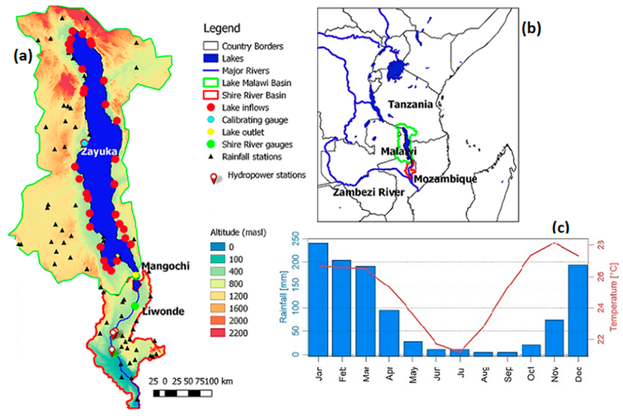
Figure 1. (a) The Lake Malawi and Shire River Basins, (b) their location in the Great Rift Valley in southeastern Africa and (c) the mean annual cycles of precipitation and temperature in the study area.
Hydrology 07 00054 g001
Figure 2. Monthly lake level (from 1899 to 2018), lake outflow at Mangochi (1976 to 2004) and Shire River discharge at Liwonde (1948 to 2008).
Hydrology 07 00054 g002
Figure 3. Conceptual overview of the hydrological model cascade applied in this study. The Mesoscale Hydrological Model mHM is used to dynamically simulate hydrological flows for the upstream Lake Malawi Basin (Upstream Lake Malawi Basin Model, ULMBM) and the upper and middle Shire River Basin (Shire River Model, SRM). A lake model (Lake Malawi Model, LMM) has been developed to dynamically simulate the water budget, lake levels and outflow dynamics of Lake Malawi. The models are driven by meteorological forcings, and model outputs from previous steps in the model cascade serve as inputs for lower model chain components. The hydropower production model (HPP) estimates hydropower generation on the Shire River.
Hydrology 07 00054 g003
Figure 4. Simulated vs. observed hydrographs for the calibration and verification periods (columns) obtained by the mHM for the Upstream Lake Malawi Basin Model (ULMBM) and the Shire River Model (SRM) (rows).
Hydrology 07 00054 g004
Figure 5. Simulated time series and boxplots for lake level (upper) and lake outflow (bottom), as simulated by the Lake Malawi Model (LMM) for the period 1976–2013 against observations.
Hydrology 07 00054 g005
Figure 6. The sensitivity of lake level (a,b) and outflow (c,d) to systematical changes in temperature with constant Po (column 1) and precipitation with constant To (column 2) based on Equations (8) and (9). Green lines in a and b mark the effective lake level of 470.8 m a.s.l. (i.e., No Outflow Level, NOL), while in c and d, green lines mark the flow required for maximum hydropower generation (170 m3/s) (i.e., Maximum Flow For Hydropower Productivity, MFHPP). Black curves in each plot mark the reference simulations (i.e., with no changes in T and P).
Hydrology 07 00054 g006
Figure 7. Climate change signals for temperature (left) and precipitation (right) as projected by an ensemble of 20 GCM–RCM combinations from the CORDEX Africa project based on the RCP4.5 and RCP8.5 for a near (2021–2050) and far future (2071–2100) period with reference to the 1976 to 2005 period.
Hydrology 07 00054 g007
Figure 8. Response surfaces showing absolute (in m a.s.l., (a)) and relative (deviation from reference level, (b)) changes in the water level of Lake Malawi as simulated by the ULMBM and the LMM using systematically perturbed precipitation (y-axis) and temperature (x-axis) data as input. The points added to the response surface indicate the hydro-climatological change as projected by the 20 GCM–RCM combinations indicated in Table 2. The different symbols refer to different periods and scenarios (rectangles/circles: RCP4.5 near/far future; triangles/diamonds: RCP8.5 near/far future). The colored symbols reflect the mean of the climate model ensemble for the respective periods and scenarios (same color code as in Figure 7). Pixels marked by an “X” indicate combinations of ΔT and ΔP where outflow from Lake Malawi temporally ceases (i.e., lake level temporally falls below 470.8 m a.s.l.). R is the reference pixel (ΔT = 0; ΔP = 0).
Hydrology 07 00054 g008
Figure 9. Same as Figure 8 but for mean discharge at Liwonde gauge generated with systematically perturbed meteorological observation data as input to the hydrological model chain. Absolute (in m3/s, (a)) and relative (in % deviation from reference mean discharge, (b) mean changes).
Hydrology 07 00054 g009
Figure 10. Same as Figure 8 but for (a) absolute and (b) relative changes in mean daily produced electricity and (c) the number of days with hydropower productivity below 346 MW (hydropower reliability) summarized for all hydropower plants along the middle Shire River. Hydropower productivity is inferred from discharge simulations by the hydrological model chain driven by systematically perturbed meteorological input data.
Hydrology 07 00054 g010
Table 1. The seven hydropower stations on the Shire River in Malawi in 2020 (From http://www.egenco.mw/page.php?slug=power-stations (official site of Electricity Generating Company, EGENCO, accessed on 1 February 2020)).
StationLatitudeLongitudeElevation (m.a.s.l.)Installed Hydroelectrical Power, HEP (MW)Net Hydraulic Head (m)
Nkula A and B−15.526134.82~34612455.2
Tedzani I, II and III−15.559434.7772~29192.744.8
Kapichira I and II−15.901134.7531~112129.654
Total 346.3
Table 2. Matrix of CORDEX Africa models used in the study. The matrix consists of ten Global Climate Models (GCMs) and five Regional Climate Models (RCMs) from five centers: Swedish Meteorological and Hydrological Institute (SMHI), Sweden, Max Planck Institute (MPI), Germany, The Royal Netherlands Meteorological Institute (KNMI), Netherlands, The Danish Meteorological Institute (DMI), Denmark, and Climate Limited-Area Modeling Community (CLM), international.
RCMsRCA4-XXXXXXXXXX-SMHIClimate Centres
REMO2015- X -MPI
REMO2009- XX -MPI
RACMO22T- X X-KNMI
HIRHAM5- X -DMI
CCLM-4-8-17-XXX X-CLM
CNRM-CM5 -EC-EARTH -MPI-ESM-LR -CanESM2 -CSIRO-Mk3.6.0 -IPSL-CM5A-MIROC5- Nor-ESM1-M -GFDL-ESM2M-HAdGEM2-ES-
GCMs
Table 3. Summary of the GCM–RCM results. Ensemble mean changes in temperature, precipitation, lake level, flow, electricity production and electricity reliability compared to the reference period (1976–2005).
Period2021–20502071–2100
ScenariosRCP4.5RCP8.5RCP4.5RCP8.5
Ensemble ChangeRangeEnsemble ChangeRangeEnsemble ChangeRangeEnsemble ChangeRange
Temperature Mean Change (° Celsius)+1.32+0.98, +1.85+1.55+0.99, +2.12+2.3+1.8, +3.2+4.2+3.4, +5
Precipitation Mean Change (%)−2.2−11, +3−0.63−14, +26−4.6−15, +6−7.1−16, +3
Lake Level Mean Change (m)−1.1−1.9, +0.5−0.5−2.1, +3.3−1.5−2.2, +0.2−2.1−2.4, +0.2
Flow Mean Change at Liwonde (%)−49−70, +24−23−76, +203−59−78, +7−75−82, +4
Electricity Production Mean Change (%)−2.5−13, +0.1−0.7−24, +0.1−5−29, +0.07−24−38, −0.07
Electricity Reliability Mean (Days) 146190, 016264, 089284, 3259318, 4
1 Days without maximum electricity production per year.