Relationship between Ocean-Atmospheric Climate Variables and Regional Streamflow of the Conterminous United States


Abstract
:1. Introduction
- The association between conterminous U.S. streamflow and climate variables of the Pacific and Atlantic Oceans and to analyze the driving mechanism of streamflow variability due to these climate variables.
- The correlation between regional streamflow and three important predefined indices, namely, the ENSO, PDO, and AMO.
2. Study Area and Data
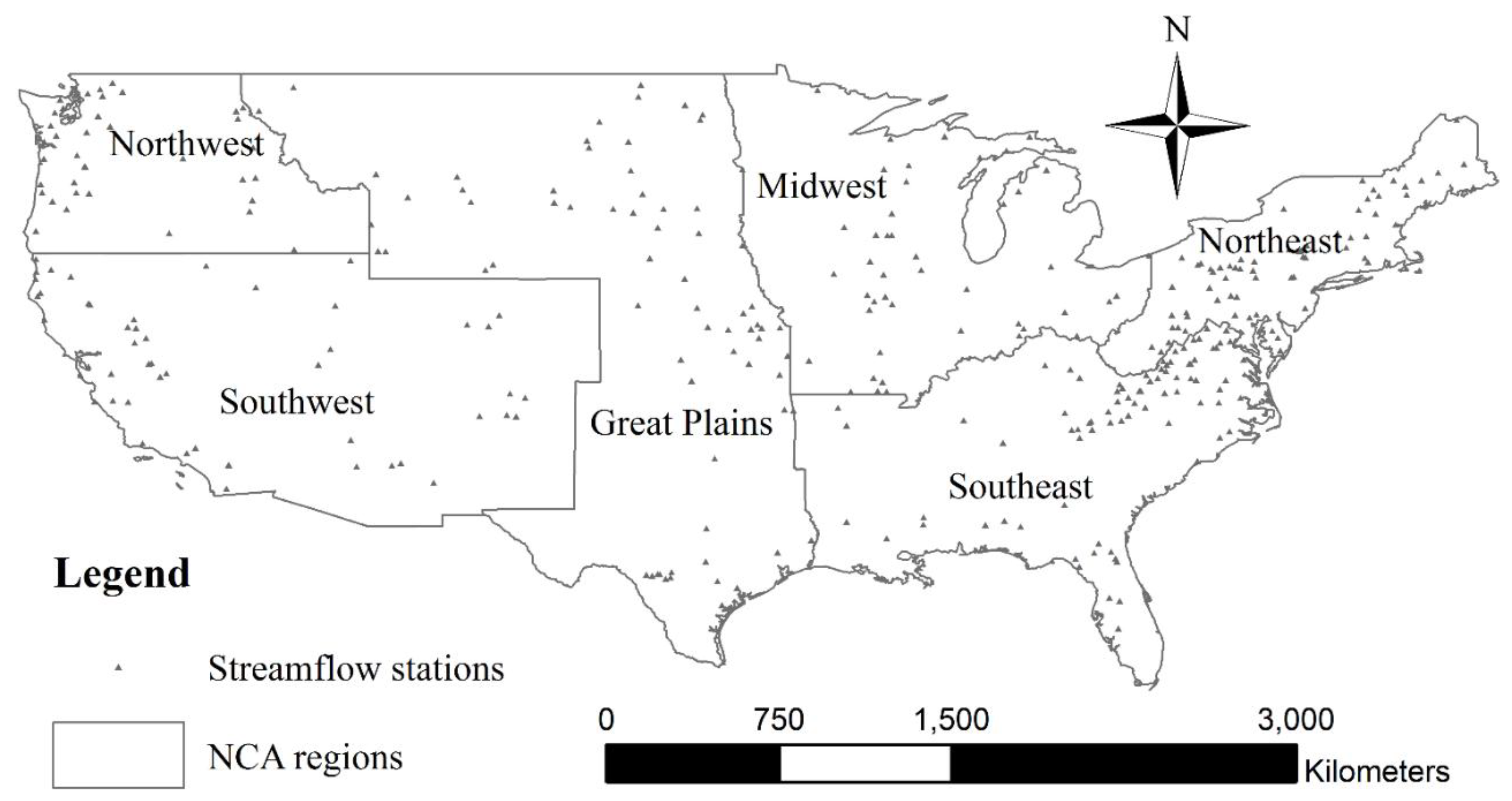
2.1. Study Area
2.2. Data
2.2.1. Streamflow Data
2.2.2. Climate Variability Data
3. Methodology
3.1. Singular Value Decomposition
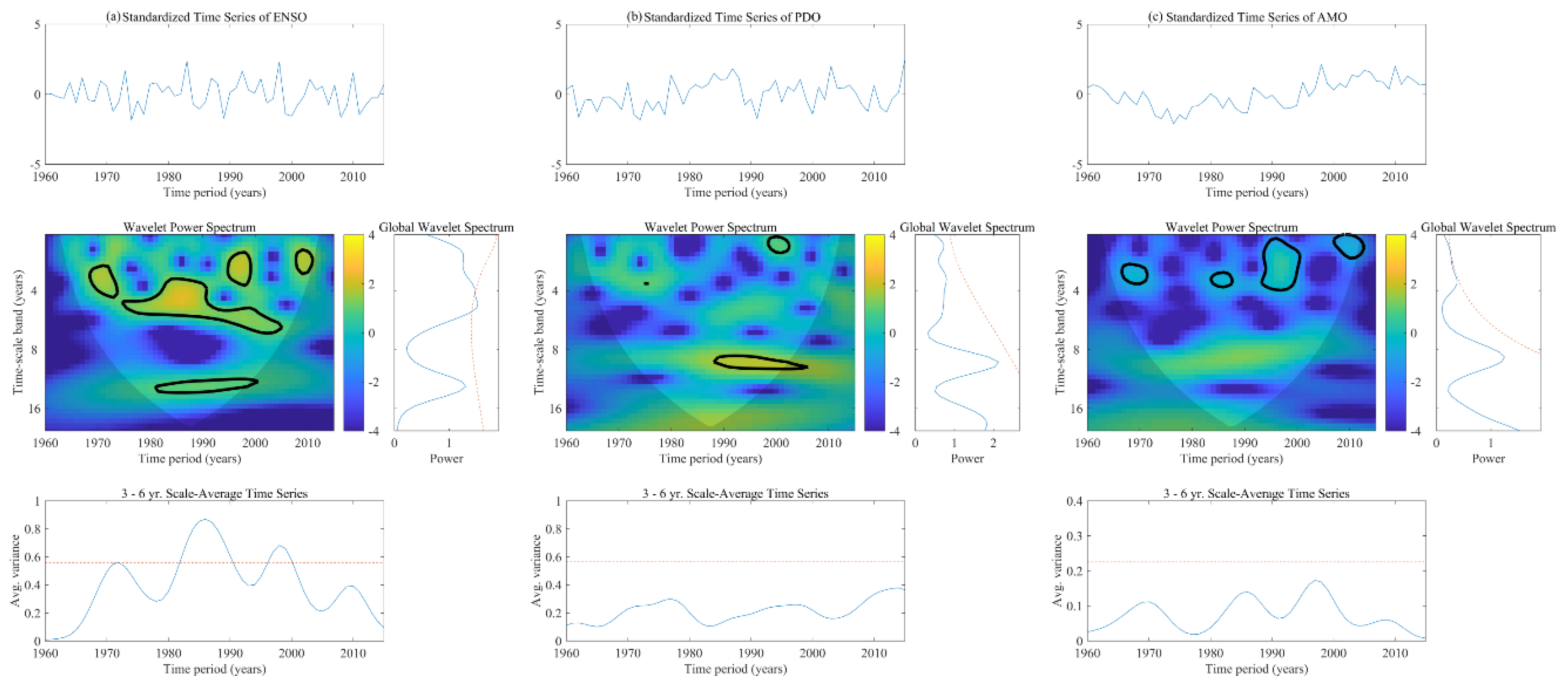
3.2. Continuous Wavelet Transform and its Derivatives
4. Results and Discussion
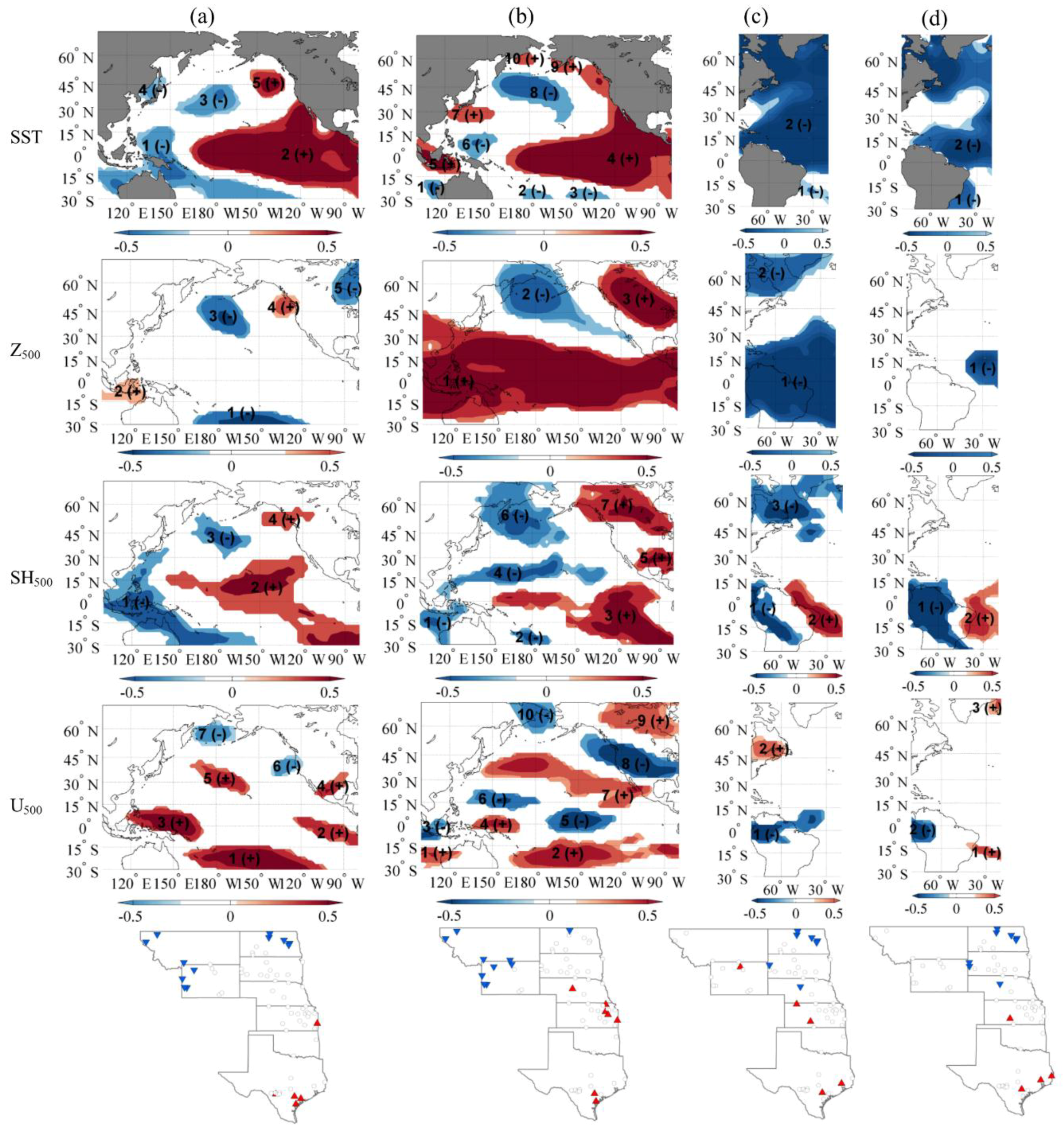
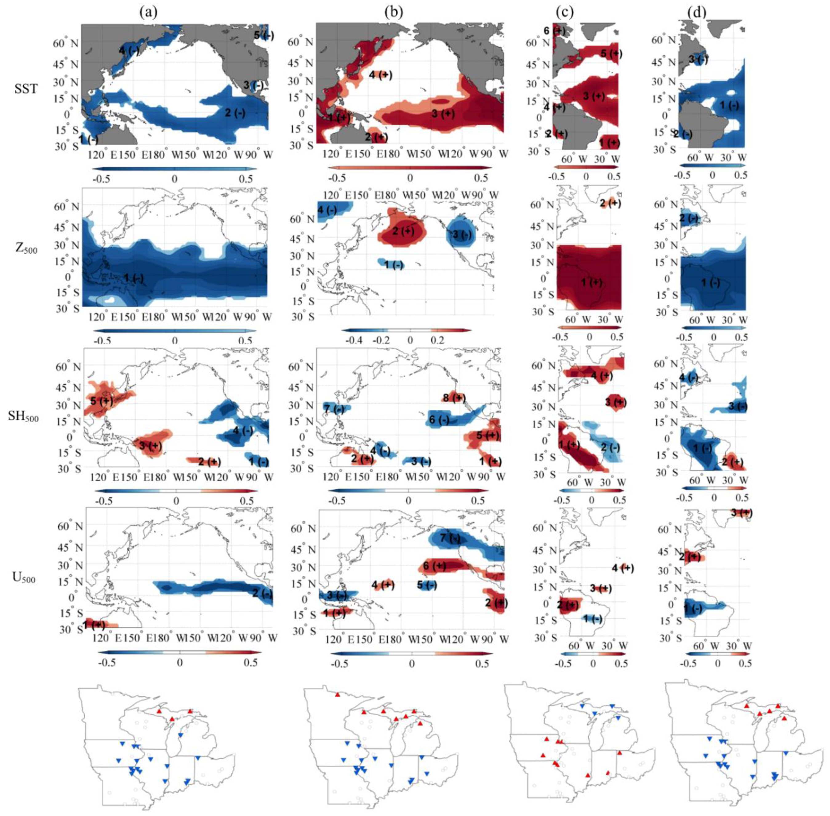
4.1. SVD Analysis
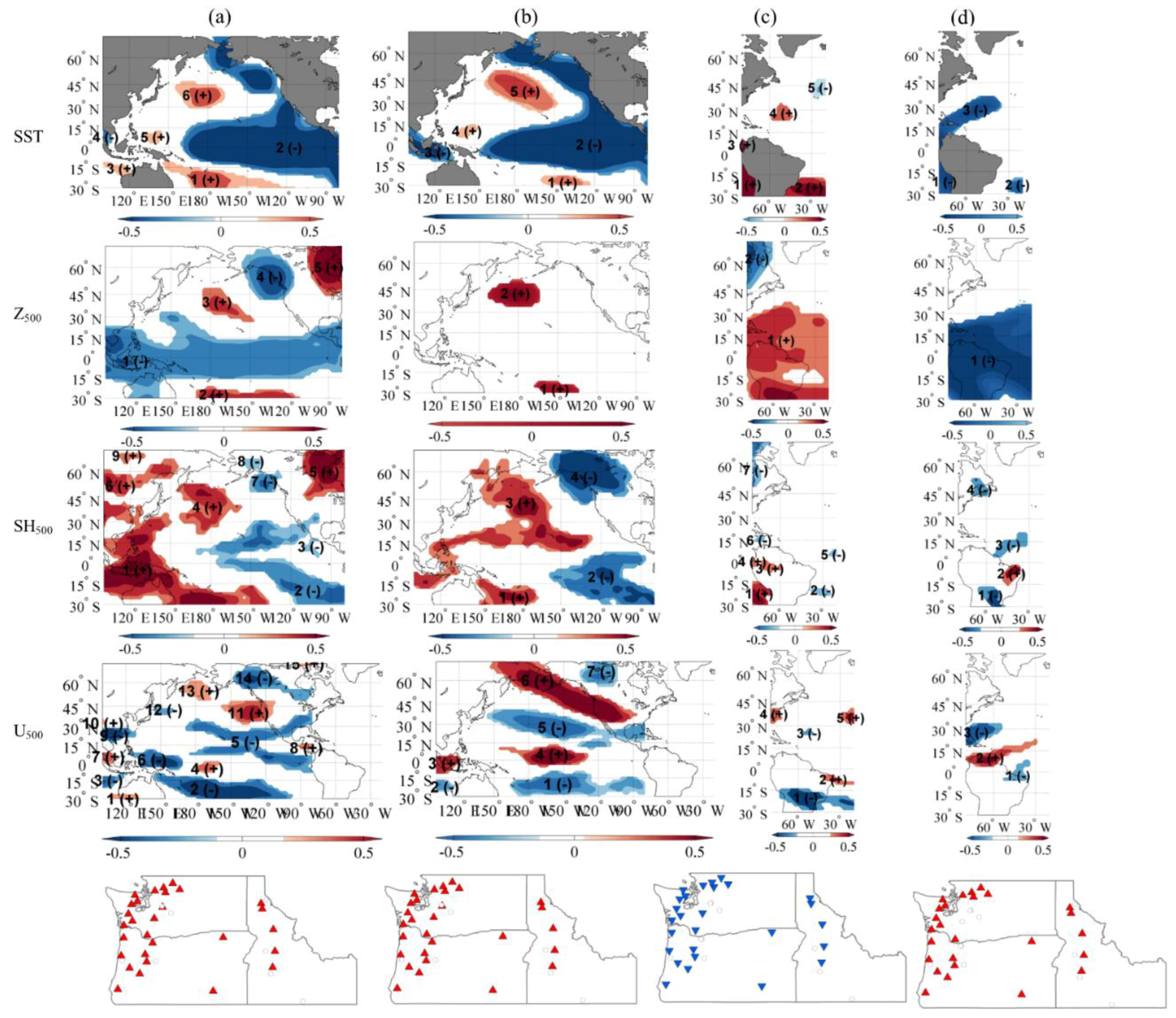
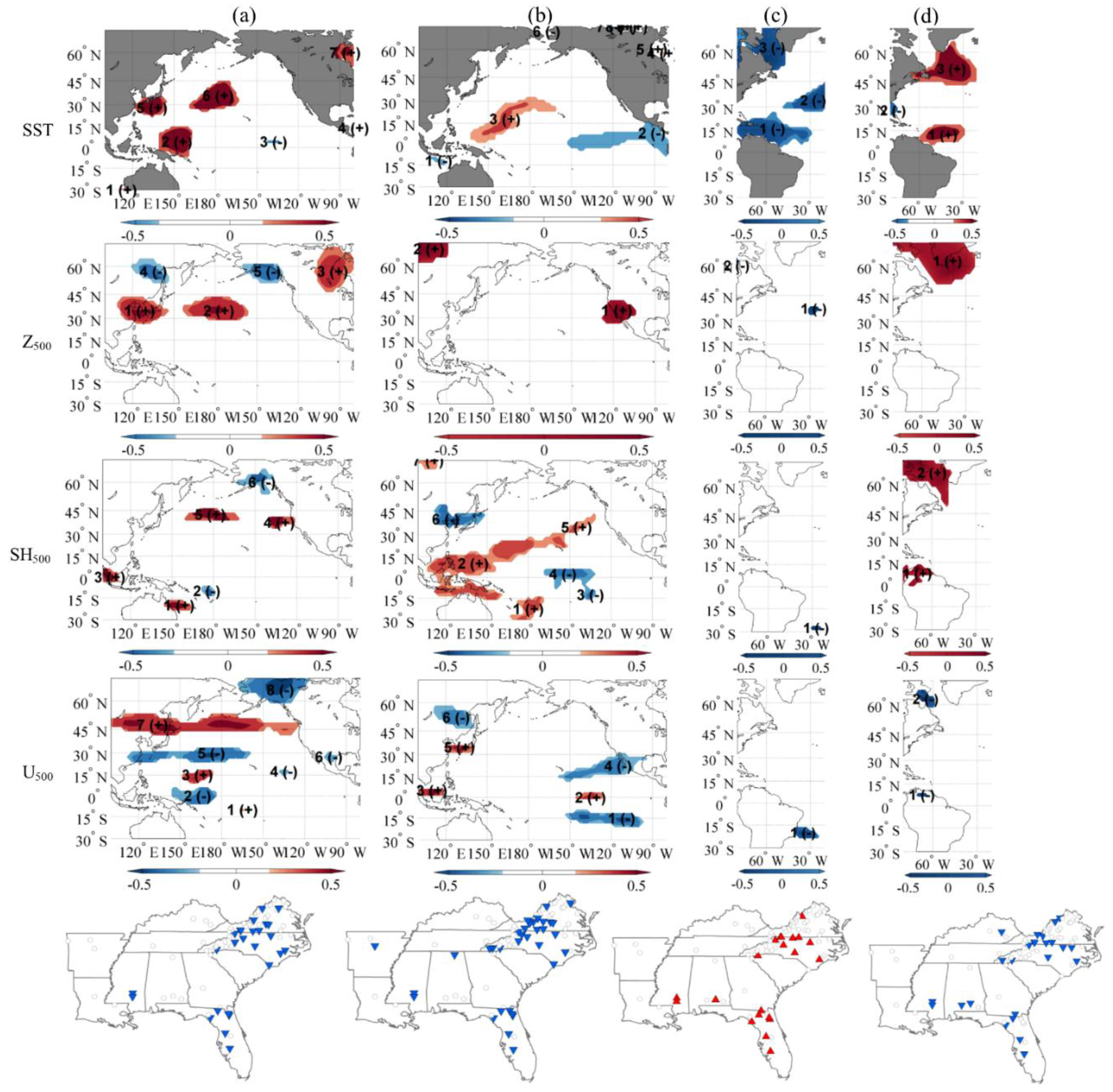
4.1.1. Great Plains
4.1.2. Midwest
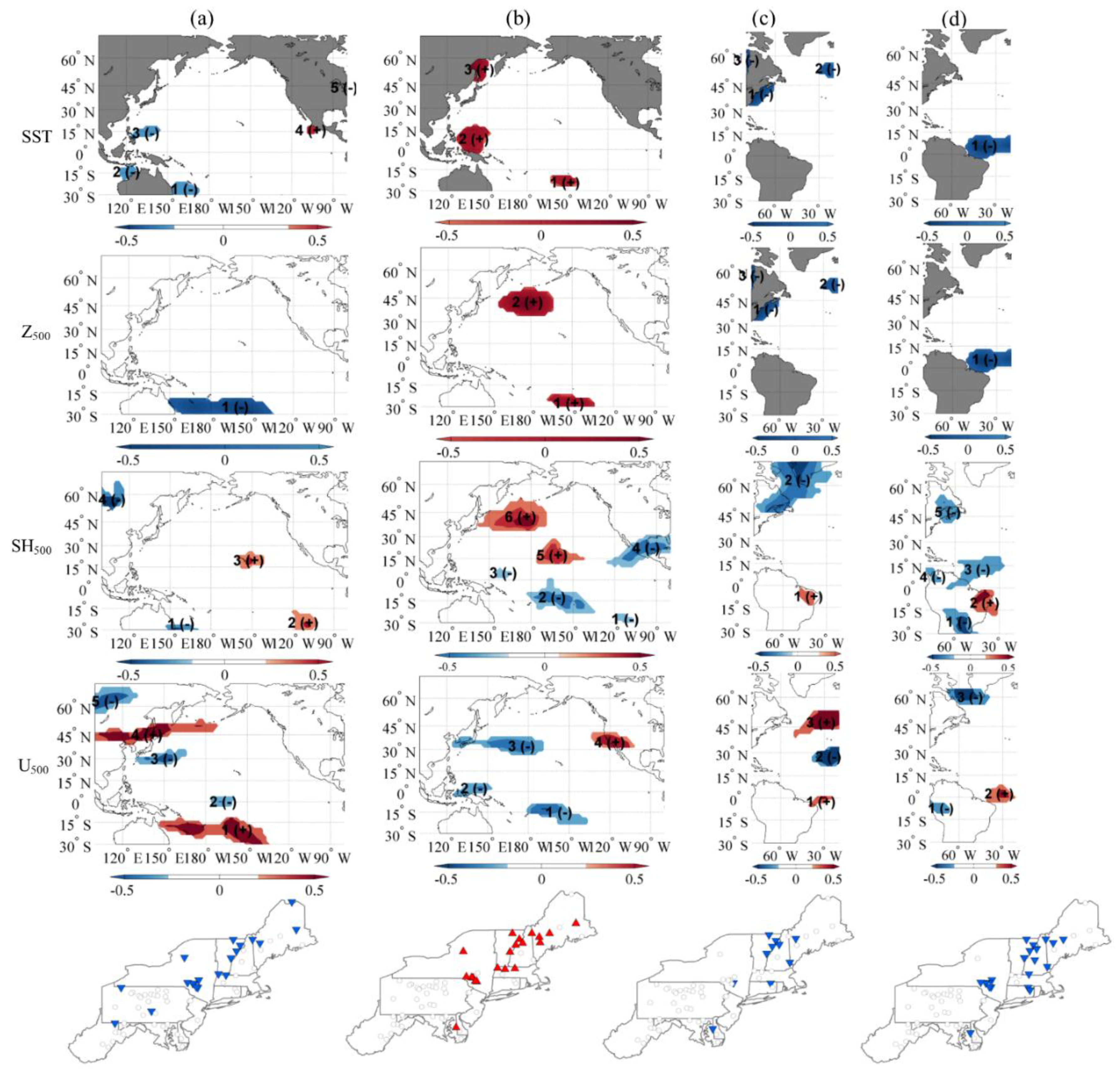
4.1.3. Northeast
4.1.4. Northwest
4.1.5. Southeast
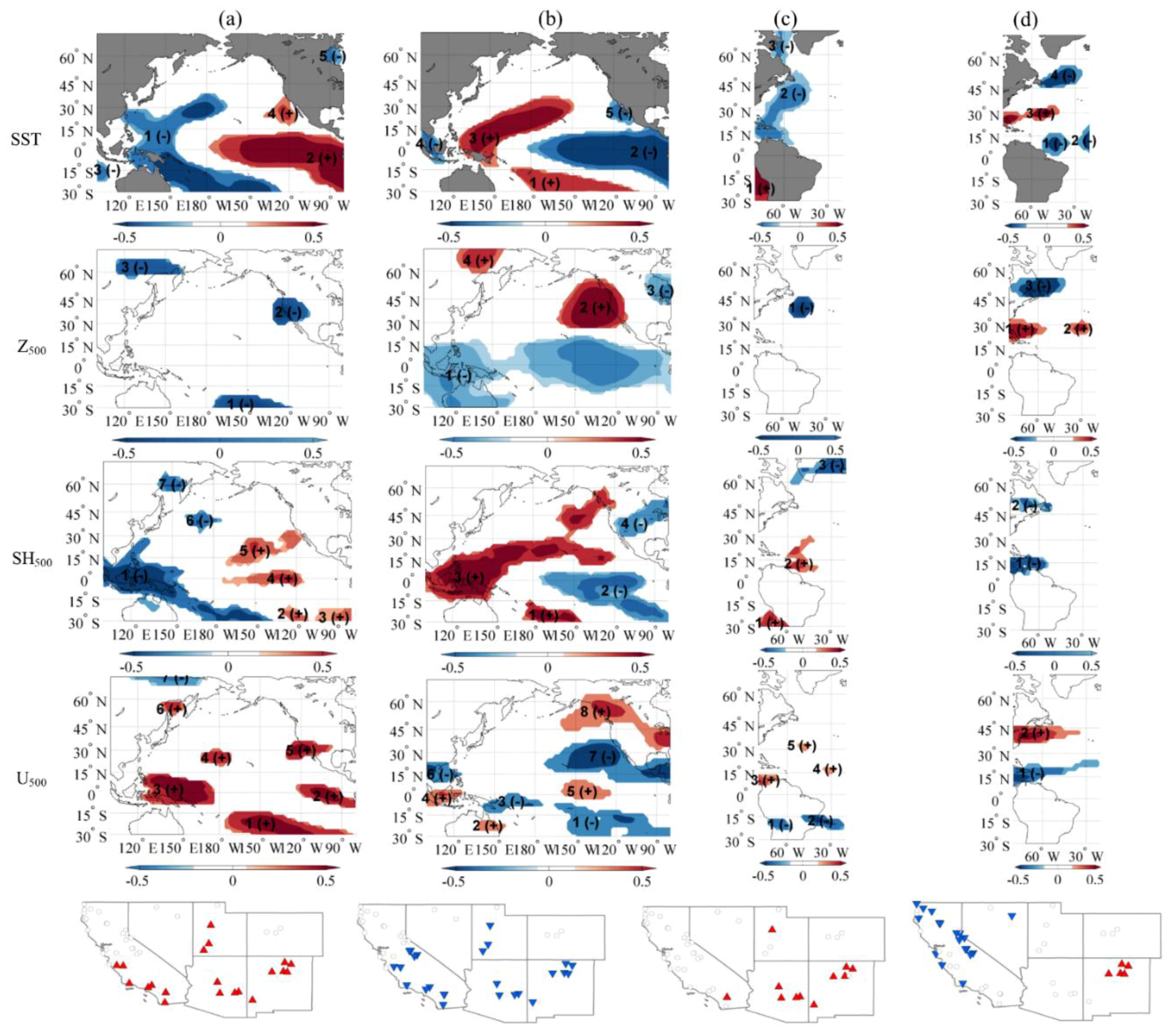
4.1.6. Southwest
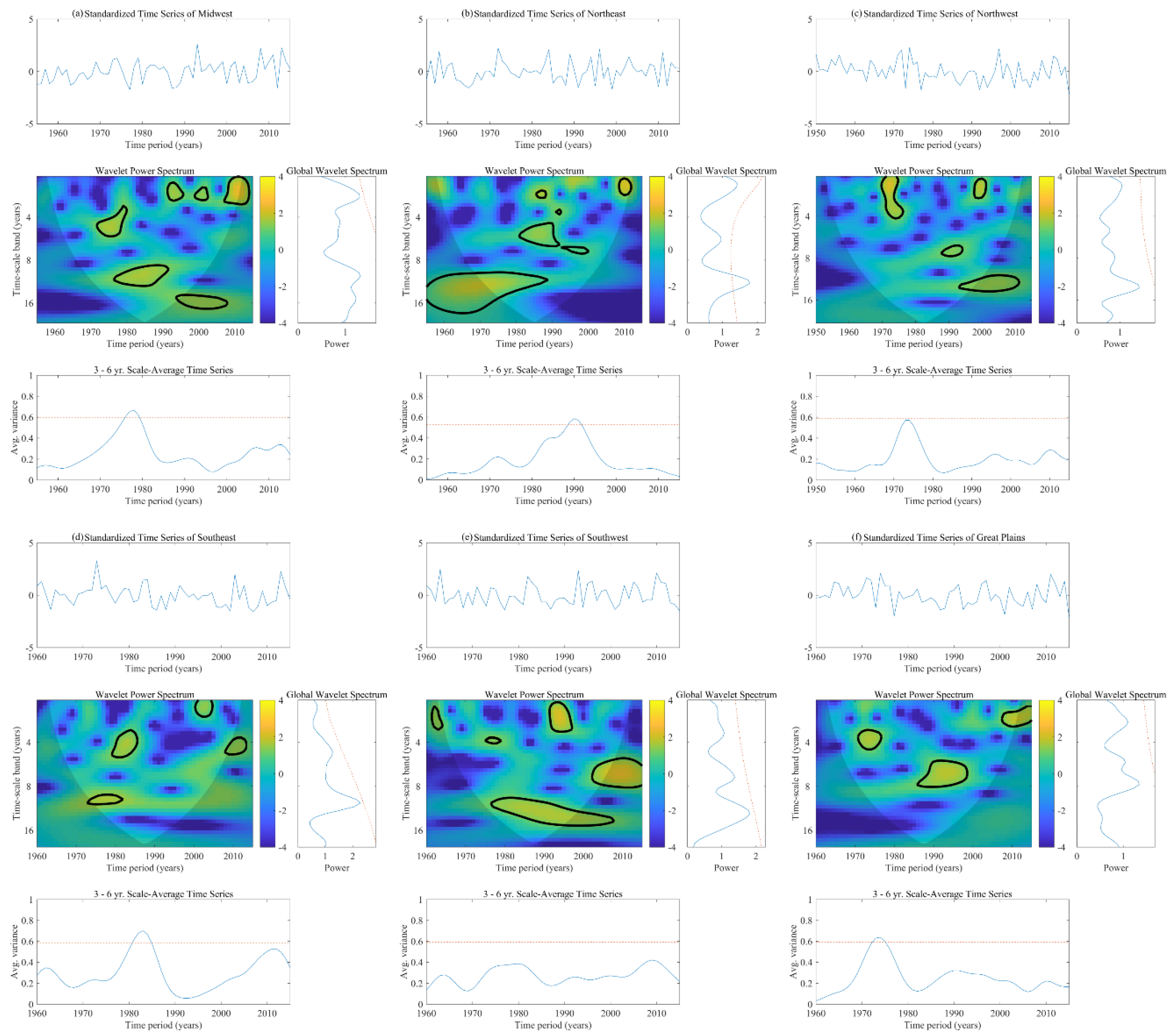
4.2. CWT Analysis
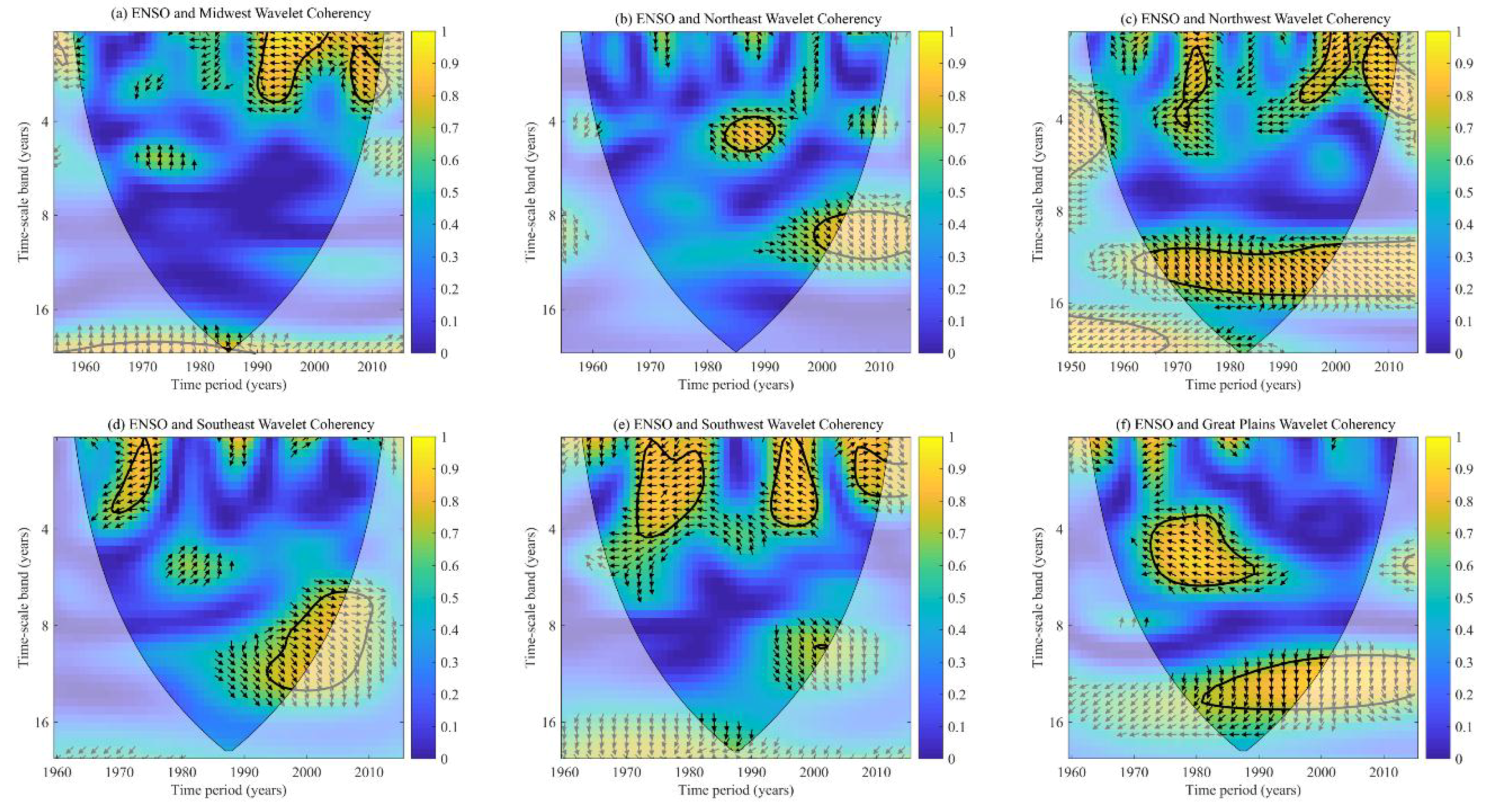
4.2.1. Correlation between ENSO and Regional Streamflow
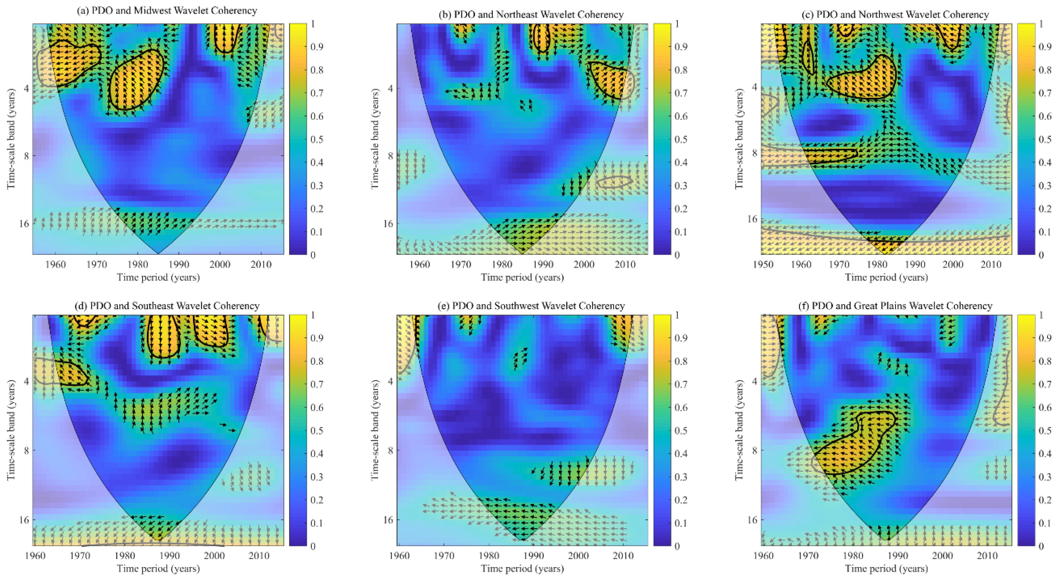
4.2.2. Correlation between PDO and Regional Streamflow
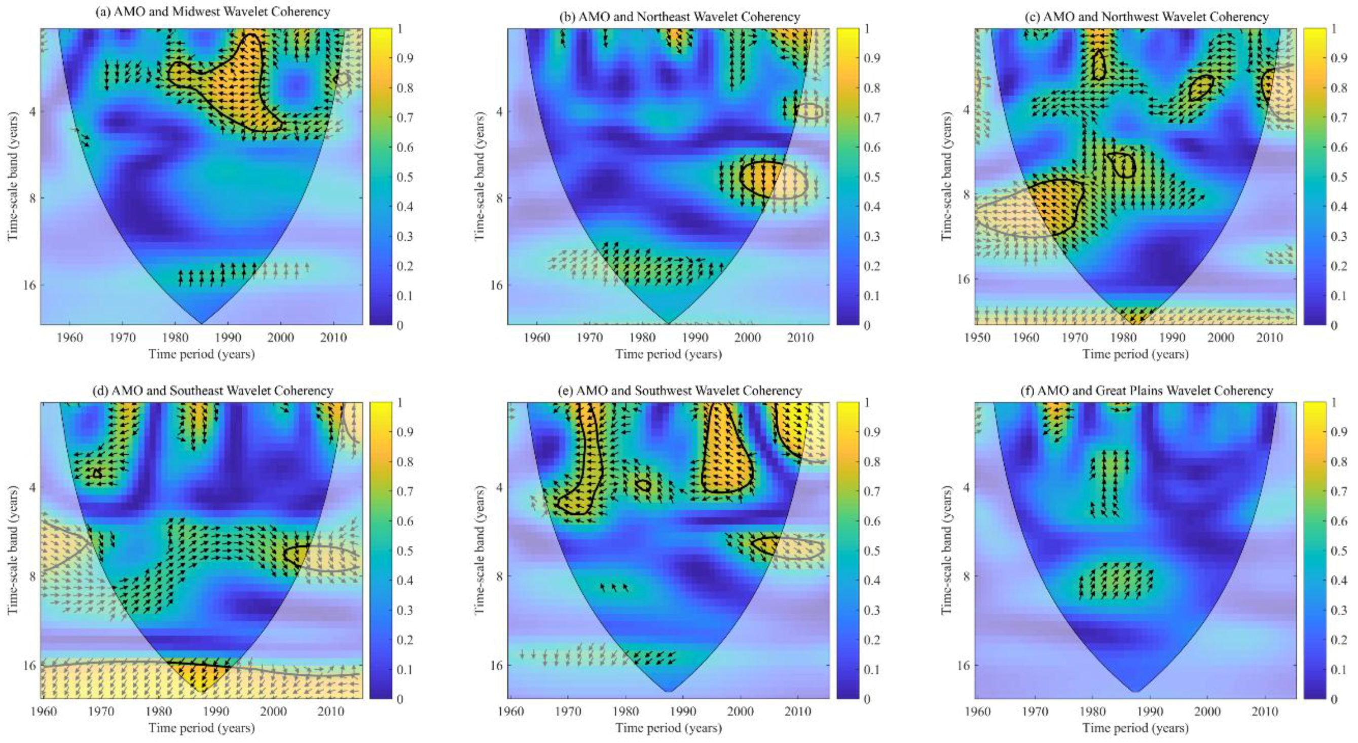
4.2.3. Correlation between AMO and Regional Streamflow
5. Conclusions
- The warming phase of SST in the ENSO-like region was found to be positively correlated with the majority of streamflow variability in the Great Plains, Midwest, and Southwest regions, while the warming phase of SST in the ENSO-like region showed a negative correlation with the Northwest streamflow.
- Both the Pacific and the Atlantic SST, Z500, and SH500 did not show any distinct influence on the streamflow variability of the Northeast and the Southeast regions.
- The Northwest streamflow was highly correlated with both ENSO and PDO while the Southeast streamflow showed the highest correlation with AMO among the regions.
- All the possible teleconnections of the climate variables with conterminous U.S. streamflow were presented. The consistently teleconnected regions could be utilized in developing long lead-time streamflow forecasting in the regional level.
- SST, Z500, SH500, and U500 were utilized together to find the coupled relationship with streamflow. SH500 and U500 data have received little research attention in the previous studies.
- A comprehensive analysis using both SVD and wavelet approach helped in understanding the time-lagged relationship between U.S. streamflow and entire Pacific/Atlantic climate variables along with predefined indices.
Author Contributions
Funding
Acknowledgments
Conflicts of Interest
Abbreviations
| NCA | National Climate Assessment |
| SST | Sea Surface Temperature |
| Z500 | Geopotential Height at 500 mbar pressure |
| SH500 | Specific Humidity at 500 mbar pressure |
| U500 | East-West Zonal Wind at 500 mbar pressure |
References
- Mach, K.; Mastrandrea, M. Climate Change 2014: Impacts, Adaptation, and Vulnerability; Field, C.B., Barros, V.R., Eds.; Cambridge University Press: Cambridge, UK, 2014. [Google Scholar]
- Gleick, P.H. Climate change, hydrology, and water resources. Rev. Geophys. 1989, 27, 329–344. [Google Scholar] [CrossRef]
- Middelkoop, H.; Daamen, K.; Gellens, D.; Grabs, W.; Kwadijk, J.C.; Lang, H.; Wilke, K. Impact of climate change on hydrological regimes and water resources management in the Rhine basin. Clim. Chang. 2001, 49, 105–128. [Google Scholar] [CrossRef]
- Miles, E.L.; Snover, A.K.; Hamlet, A.F.; Callahan, B.; Fluharty, D. Pacific Northwest regional assessment: The impacts of climate variability and climate change on the water resources of the Columbia River Basin. J. Am. Water Resour. Assoc. 2000, 36, 399–420. [Google Scholar] [CrossRef]
- Tamaddun, K.A.; Kalra, A.; Ahmad, S. Wavelet analyses of western US streamflow with ENSO and PDO. J. Water Clim. Chang. 2017, 8, 26–39. [Google Scholar] [CrossRef]
- Redmond, K.T.; Koch, R.W. Surface climate and streamflow variability in the western United States and their relationship to large-scale circulation indices. Water Resour. Res. 1991, 27, 2381–2399. [Google Scholar] [CrossRef]
- Cayan, D.R.; Webb, R.H. El Niño/southern oscillation and streamflow in the western United States. In El Niño, Historical and Paleoclimatic Aspects of the Southern Oscillation; Diaz, H.F., Markgraf, V., Eds.; Cambridge University Press: Cambridge, UK, 1992. [Google Scholar]
- Dettinger, M.D.; Diaz, H.F. Global characteristics of stream flow seasonality and variability. J. Hydrometeorol. 2000, 1, 289–310. [Google Scholar] [CrossRef]
- Wallace, J.M.; Gutzler, D.S. Teleconnections in the geopotential height field during the Northern Hemisphere winter. Mon. Weather. Rev. 1981, 109, 784–812. [Google Scholar] [CrossRef]
- Kahya, E.; Dracup, J.A. US streamflow patterns in relation to the El Niño/Southern Oscillation. Water Resour. Res. 1993, 29, 2491–2503. [Google Scholar] [CrossRef]
- Barlow, M.; Nigam, S.; Berbery, E.H. ENSO, Pacific decadal variability, and US summertime precipitation, drought, and stream flow. J. Clim. 2001, 14, 2105–2128. [Google Scholar] [CrossRef]
- Webster, P.J.; Magana, V.O.; Palmer, T.N.; Shukla, J.; Tomas, R.A.; Yanai, M.U.; Yasunari, T. Monsoons: Processes, predictability, and the prospects for prediction. J. Geophys. Res. Oceans 1998, 103, 14451–14510. [Google Scholar] [CrossRef] [Green Version]
- Ward, P.J.; Beets, W.; Bouwer, L.M.; Aerts, J.C.; Renssen, H. Sensitivity of river discharge to ENSO. Geophys. Res. Lett. 2010, 37. [Google Scholar] [CrossRef] [Green Version]
- Ropelewski, C.F.; Halpert, M.S. Global and regional scale precipitation patterns associated with the El Niño/Southern Oscillation. Mon. Weather Rev. 1987, 115, 1606–1626. [Google Scholar] [CrossRef]
- Trenberth, K.E.; Fasullo, J. Water and energy budgets of hurricanes and implications for climate change. J. Geophys. Res. Atmospheres, 2007, 112. [Google Scholar] [CrossRef] [Green Version]
- Enfield, D.B.; Mestas-Nuñez, A.M.; Trimble, P.J. The Atlantic multidecadal oscillation and its relation to rainfall and river flows in the continental US. Geophys. Res. Lett. 2001, 28, 2077–2080. [Google Scholar] [CrossRef]
- McCabe, G.J.; Palecki, M.A.; Betancourt, J.L. Pacific and Atlantic Ocean influences on multidecadal drought frequency in the United States. Proc. Natl. Acad. Sci. USA 2004, 101, 4136–4141. [Google Scholar] [CrossRef] [PubMed] [Green Version]
- Grantz, K.; Rajagopalan, B.; Clark, M.; Zagona, E. A technique for incorporating large-scale climate information in basin-scale ensemble streamflow forecasts. Water Resour. Res. 2005, 41. [Google Scholar] [CrossRef]
- Tootle, G.A.; Piechota, T.C. Relationships between Pacific and Atlantic ocean sea surface temperatures and US streamflow variability. Water Resour. Res. 2006, 42. [Google Scholar] [CrossRef]
- Pascolini-Campbell, M.; Seager, R.; Pinson, A.; Cook, B.I. Covariability of climate and streamflow in the Upper Rio Grande from interannual to interdecadal timescales. J. Hydrol. Reg. Stud. 2017, 13, 58–71. [Google Scholar] [CrossRef]
- Corte-Real, J.; Zhang, X.; Wang, X. Large-scale circulation regimes and surface climatic anomalies over the Mediterranean. Int. J. Climatol. 1995, 15, 1135–1150. [Google Scholar] [CrossRef]
- Pathak, P.; Kalra, A.; Lamb, K.W.; Miller, W.P.; Ahmad, S.; Amerineni, R.; Ponugoti, D.P. Climatic variability of the Pacific and Atlantic Oceans and western US snowpack. Int. J. Climatol. 2018, 38, 1257–1269. [Google Scholar] [CrossRef]
- Bretherton, C.S.; Smith, C.; Wallace, J.M. An intercomparison of methods for finding coupled patterns in climate data. J. Clim. 1992, 5, 541–560. [Google Scholar] [CrossRef]
- Praus, P. Water quality assessment using SVD-based principal component analysis of hydrological data. Water SA 2005, 31, 417–422. [Google Scholar] [CrossRef]
- Wallace, J.M.; Smith, C.; Bretherton, C.S. Singular value decomposition of wintertime sea surface temperature and 500-mb height anomalies. J. Clim. 1992, 5, 561–576. [Google Scholar] [CrossRef]
- Abdi, H. Singular value decomposition (SVD) and generalized singular value decomposition. In Encyclopedia of Measurement and Statistics; Salkind, N.J., Ed.; Sage: Thousand Oaks, CA, USA, 2007. [Google Scholar]
- Oubeidillah, A.A.; Tootle, G.A.; Moser, C.; Piechota, T.; Lamb, K. Upper Colorado River and Great Basin streamflow and snowpack forecasting using Pacific oceanic–atmospheric variability. J. Hydrol. 2011, 410, 169–177. [Google Scholar] [CrossRef]
- Sagarika, S.; Kalra, A.; Ahmad, S. Interconnections between oceanic–atmospheric indices and variability in the US streamflow. J. Hydrol. 2015, 525, 724–736. [Google Scholar] [CrossRef]
- Shams, M.S.; Anwar, A.F.; Lamb, K.W.; Bari, M. Relating ocean-atmospheric climate indices with Australian river streamflow. J. Hydrol. 2018, 556, 294–309. [Google Scholar] [CrossRef]
- Sang, Y.F. A review on the applications of wavelet transform in hydrology time series analysis. Atmos. Res. 2013, 122, 8–15. [Google Scholar] [CrossRef]
- Lau, K.M.; Weng, H. Climate signal detection using wavelet transform: How to make a time series sing. Bull. Am. Meteorol. Soc. 1995, 76, 2391–2402. [Google Scholar] [CrossRef]
- Tamaddun, K.A.; Kalra, A.; Bernardez, M.; Ahmad, S. Multi-scale correlation between the western US snow water equivalent and ENSO/PDO using wavelet analyses. Water Resour. Manag. 2017, 31, 2745–2759. [Google Scholar] [CrossRef]
- Coulibaly, P.; Baldwin, C.K. Nonstationary hydrological time series forecasting using nonlinear dynamic methods. J. Hydrol. 2005, 307, 164–174. [Google Scholar] [CrossRef]
- Labat, D. Cross wavelet analyses of annual continental freshwater discharge and selected climate indices. J. Hydrol. 2010, 385, 269–278. [Google Scholar] [CrossRef]
- Lins, H.F. USGS Hydro-Climatic Data Network 2009 (HCDN-2009): U.S. Geological Survey Fact Sheet 2012-3047; U.S. Geological Survey: Reston, VA, USA, 2012.
- Smith, T.M.; Reynolds, R.W.; Peterson, T.C.; Lawrimore, J. Improvements to NOAA’s historical merged land—Ocean surface temperature analysis (1880–2006). J. Clim. 2008, 21, 2283–2296. [Google Scholar] [CrossRef]
- Kalnay, E.; Kanamitsu, M.; Kistler, R.; Collins, W.; Deaven, D.; Gandin, L.; Iredell, M.; Saha, S.; White, G.; Woollen, J.; et al. The NCEP/NCAR 40-year reanalysis project. Bull. Am. Meteorol. Soc. 1996, 77, 437–471. [Google Scholar] [CrossRef]
- Torrence, C.; Compo, G.P. A practical guide to wavelet analysis. Bull. Am. Meteorol. Soc. 1998, 79, 61–78. [Google Scholar] [CrossRef]
- Torrence, C.; Webster, P.J. Interdecadal changes in the ENSO–monsoon system. J. Clim. 1999, 12, 2679–2690. [Google Scholar] [CrossRef]
- Labat, D. Recent advances in wavelet analyses: Part 1. A review of concepts. J. Hydrol. 2005, 314, 275–288. [Google Scholar] [CrossRef]
- Liu, Y.; Liang, S.X.; Weisberg, R.H. Rectification of the bias in the wavelet power spectrum. J. Atmos. Ocean. Tech. 2007, 24, 2093–2102. [Google Scholar] [CrossRef]
- Foufoula-Georgiou, E.; Kumar, P.; Mukerji, T.; Mavko, G. Wavelets in geophysics. Pure Appl. Geophys. 1995, 145, 374–375. [Google Scholar]
- Percival, D.B.; Walden, A.T. Wavelet Methods for Time Series Analysis; Cambridge University Press: Cambridge, UK, 2006. [Google Scholar]
- Jevrejeva, S.; Moore, J.C.; Grinsted, A. Influence of the Arctic Oscillation and El Niño-Southern Oscillation (ENSO) on ice conditions in the Baltic Sea: The wavelet approach. J. Geophys. Res. Atmos. 2003, 108. [Google Scholar] [CrossRef] [Green Version]
- Grinsted, A.; Moore, J.C.; Jevrejeva, S. Application of the cross wavelet transform and wavelet coherence to geophysical time series. Nonlinear Process. Geophys. 2004, 11, 561–566. [Google Scholar] [CrossRef] [Green Version]
- Wallace, J.M.; Zhang, Y.; Lau, K.H. Structure and seasonality of interannual and interdecadal variability of the geopotential height and temperature fields in the Northern Hemisphere troposphere. J. Clim. 1993, 6, 2063–2082. [Google Scholar] [CrossRef]
- Alexander, M.A.; Bladé, I.; Newman, M.; Lanzante, J.R.; Lau, N.C.; Scott, J.D. The atmospheric bridge: The influence of ENSO teleconnections on air–sea interaction over the global oceans. J. Clim. 2002, 15, 2205–2231. [Google Scholar] [CrossRef]
- Rajagopalan, B.; Cook, E.; Lall, U.; Ray, B.K. Spatiotemporal variability of ENSO and SST teleconnections to summer drought over the United States during the twentieth century. J. Clim. 2000, 13, 4244–4255. [Google Scholar] [CrossRef]
- Dunnell, K.L.; Travers, S.E. Shifts in the flowering phenology of the northern Great Plains: Patterns over 100 years. Am. J. Bot. 2011, 98, 935–945. [Google Scholar] [CrossRef] [PubMed] [Green Version]
- Wang, H.; Ting, M. Covariabilities of winter US precipitation and Pacific sea surface temperatures. J. Clim. 2000, 13, 3711–3719. [Google Scholar] [CrossRef]
- Zhang, Y.; Wallace, J.M.; Battisti, D.S. ENSO-like interdecadal variability: 1900–93. J. Clim. 1997, 10, 1004–1020. [Google Scholar] [CrossRef]
- Chang, P.; Ji, L.; Li, H. A decadal climate variation in the tropical Atlantic Ocean from thermodynamic air-sea interactions. Nature 1997, 385, 516–518. [Google Scholar] [CrossRef]
- Aziz, O.A.; Tootle, G.A.; Gray, S.T.; Piechota, T.C. Identification of Pacific Ocean sea surface temperature influences of Upper Colorado River Basin snowpack. Water Resour. Res. 2010, 46. [Google Scholar] [CrossRef] [Green Version]
- Hunter, T.; Tootle, G.; Piechota, T. Oceanic-atmospheric variability and western US snowfall. Geophys. Res. Lett. 2006, 33. [Google Scholar] [CrossRef]
- Lamb, K.W.; Piechota, T.C.; Aziz, O.A.; Tootle, G.A. Basis for extending long-term streamflow forecasts in the Colorado River basin. J. Hydrol. Eng. 2010, 16, 1000–1008. [Google Scholar] [CrossRef]
- Sagarika, S.; Kalra, A.; Ahmad, S. Pacific Ocean SST and Z500 climate variability and western US seasonal streamflow. Int. J. Climatol. 2016, 36, 1515–1533. [Google Scholar] [CrossRef]


| Great Plains | Midwest | Northeast | Southeast | Southwest | Northwest |
|---|---|---|---|---|---|
| Texas | Ohio | Maine | Virginia | California | Idaho |
| Oklahoma | Indiana | Vermont | Kentucky | Nevada | Oregon |
| Kansas | Michigan | New Hampshire | Tennessee | Utah | Washington |
| Nebraska | Illinois | Massachusetts | Arkansas | Arizona | |
| South Dakota | Wisconsin | New York | Mississippi | New Mexico | |
| North Dakota | Missouri | Rhode Island | Alabama | Colorado | |
| Wyoming | Iowa | Connecticut | Louisiana | ||
| Montana | Minnesota | New Jersey | Georgia | ||
| Pennsylvania | Florida | ||||
| Maryland | South Carolina | ||||
| Delaware | North Carolina | ||||
| Washington DC | |||||
| West Virginia |
| Serial No. | NCA Regions | No. of Stations | Data Range | Total Variance Explained by FPC |
|---|---|---|---|---|
| 1 | Midwest | 45 | 1955–2015 | 49.68% |
| 2 | Northeast | 66 | 1955–2015 | 58.33% |
| 3 | Northwest | 38 | 1950–2015 | 80.10% |
| 4 | Southeast | 82 | 1960–2015 | 58.92% |
| 5 | Southwest | 50 | 1960–2015 | 71.81% |
| 6 | Great Plains | 69 | 1960–2015 | 59.77% |
| Climate Variability | Pacific Ocean | Atlantic Ocean | ||||||
|---|---|---|---|---|---|---|---|---|
| Lead-time (months) | 1 | 4 | 1 | 4 | ||||
| NCA regions | SCF (%) | NSC (%) | SCF (%) | NSC (%) | SCF (%) | NSC (%) | SCF (%) | NSC (%) |
| Great Plains | 49.8 | 3.2 | 46.7 | 3.3 | 46 | 2.8 | 59.7 | 2.9 |
| Midwest | 55.4 | 2.6 | 53.7 | 2.4 | 62.1 | 2.4 | 64.3 | 2.5 |
| Northeast | 45.6 | 1.2 | 50.8 | 1.5 | 55.7 | 1.5 | 55.8 | 1.5 |
| Northwest | 89.1 | 6.2 | 89.1 | 5.7 | 71.1 | 2.7 | 72.4 | 2.6 |
| Southeast | 53.3 | 1.9 | 49.6 | 1.9 | 59.4 | 2.2 | 66.3 | 2.3 |
| Southwest | 73.4 | 3.7 | 72.8 | 3.1 | 46.1 | 2.6 | 66.5 | 2.5 |
© 2018 by the authors. Licensee MDPI, Basel, Switzerland. This article is an open access article distributed under the terms and conditions of the Creative Commons Attribution (CC BY) license (http://creativecommons.org/licenses/by/4.0/).
Share and Cite
Bhandari, S.; Kalra, A.; Tamaddun, K.; Ahmad, S. Relationship between Ocean-Atmospheric Climate Variables and Regional Streamflow of the Conterminous United States. Hydrology 2018, 5, 30. https://doi.org/10.3390/hydrology5020030
Bhandari S, Kalra A, Tamaddun K, Ahmad S. Relationship between Ocean-Atmospheric Climate Variables and Regional Streamflow of the Conterminous United States. Hydrology. 2018; 5(2):30. https://doi.org/10.3390/hydrology5020030
Chicago/Turabian StyleBhandari, Swastik, Ajay Kalra, Kazi Tamaddun, and Sajjad Ahmad. 2018. "Relationship between Ocean-Atmospheric Climate Variables and Regional Streamflow of the Conterminous United States" Hydrology 5, no. 2: 30. https://doi.org/10.3390/hydrology5020030
APA StyleBhandari, S., Kalra, A., Tamaddun, K., & Ahmad, S. (2018). Relationship between Ocean-Atmospheric Climate Variables and Regional Streamflow of the Conterminous United States. Hydrology, 5(2), 30. https://doi.org/10.3390/hydrology5020030