Hydrological Modeling and Runoff Mitigation in an Ungauged Basin of Central Vietnam Using SWAT Model

Abstract

The A-Luoi district in Thua Thien Hue province of Vietnam is under extreme pressure from natural and anthropogenic factors. The area is ungauged and suffering from data scarcity. To evaluate the water resources availability and water management, we used Soil and Water Assessment Tools (SWAT). A multi-approach technique was used to calibrate the hydrological model. The model was calibrated in three time scales: daily, monthly and yearly by river discharge, actual evapotranspiration (ETa) and crop yield, respectively. The model was calibrated with Nash-Sutcliffe and R² coefficients greater than 0.7, in daily and monthly scales, respectively. In the yearly scale, the crop yield inside the model was calibrated and validated with Root Mean Square Error (RMSE) less than 2.4 ton/ha. The water resource components were mapped temporally and spatially. The outcomes showed that the highest mean monthly surface runoff, 323 to 369 mm, between September and November, resulted in extreme soil erosion and sedimentation. The monthly average of actual evapotranspiration was the highest in May and lowest in December. Furthermore, installing “Best Management Practices” (BMPs) reduced surface runoff in agricultural lands. However, using event-based hydrological and hydraulic models in the prediction and simulation of flooding events is recommended in further studies.

1. Introduction

Hydrological modeling of water cycle in areas with extreme events and natural hazards (e.g., flooding, droughts) is imperative for sustainable management of soil and water resources. Understanding water resources availability would help stakeholders and policymakers to plan and develop an area. There are various hydrological models that can estimate water resource availability (e.g., lumped models, physical distributed and semi-distributed models, empirical models, statistical models). Among these, semi-distributed hydrological models can simulate water balance spatially based on various soils, land uses, topography and climate conditions. One of these hydrological models is SWAT [1] which is tested in various world climates from arid and semi-arid regions [2] to humid and tropical areas [3]. Moreover, it is able to simulate water resources in large scales to regional scales. For example, Schuol et al. [4] estimated blue and green water availability in the African continent. Phuong et al. [5] evaluated the surface runoff and soil erosion in a regional area in Vietnam. One of the concerns in hydrological modeling is the uncertainty of parameters; therefore, Qiao et al. [6] used a multi-objective function to reduce this uncertainty in the SWAT model.

Surface runoff, soil erosion and flooding are the main issues in humid and tropical areas due to heavy rainfall [7]. Various researchers have studied climate variabilities and human activities on soil erosion, water quality and hydrological process [8,9].

Vietnam’s tropical region is very prone to soil erosion and surface runoff. Approximately 40% of natural areas are at risk of erosion [10]. In recent years, most of the forested areas, particularly in Central Vietnam, were converted into agricultural lands, which resulted in surface runoff and soil erosion [11]. Additionally, the hydrological behavior of watersheds in Vietnam is changing due to anthropogenic factors. The evidence of this comes from rising of soil erosion, surface runoff and floods in Central Vietnam [5]. There is no comprehensive framework to mitigate the environmental hazards in this area; therefore, we created a hydrological model of Central Vietnam with a case study in the area of A-Luoi district in Hue province.

The A-Luoi district in Central Vietnam is under high socio-economic pressure, which resulted in various natural hazards such as flooding and soil erosion. Lack of data is one of the main obstacles for policymakers in this area. The main goal of this research is to set up a hydrological model in the A-Luoi area as a representative case study of Central Vietnam and to simulate the water balance components (e.g., water yield, soil moisture, actual evapotranspiration) in order to understand the status of water resources in this area. Assessments of surface runoff, and soil erosion are the further goals of this study. We calibrated the hydrological model using multiple calibration approaches by satellite images and regionalization technique. Finally, we presented the best management practices adapted to A-Luoi area to reduce surface runoff and soil erosion.

2. Material and Methods

2.1. Study Area

The study area is a part of A-Luoi district, which is located in the center of Vietnam. The A-Luoi district consists of three watersheds. The first watershed in the west of the A-Luoi, where the main river, called the “Xe Khong River,” flows toward Laos. This watershed has an area of approximately 542 km². The second watershed is situated in the middle of A-Luoi and the main river, Song Sia River, flows into the “Tam Giang lagoon”. The watershed has an area of approximately 410 km². The third watershed in the east of A-Luoi district has an area of approximately 506 km². The river in this watershed, called “Song Huu Trach River,” flows into the “Song Huong lagoon’’ (Figure 1). We selected the second watershed as our study area, while it is the main part of A-Luoi district.

The annual rainfall in this watershed varies from 2228 mm to 5495 mm (long term climate data). According to the Soil Taxonomic classification [12], Ferralic Acrisols is the dominant soil type in this area. There are Humic Acrisols and Lithic Leptosols types in the northwestern and southeastern part of A-Luoi as well. The watershed has diverse elevations from 19 to 1777 meters above sea level from the north to the west of the basin. Figure 1 shows the study area in A-Luoi district including climate and hydrometric stations around the district.

2.2. Data Acquisition

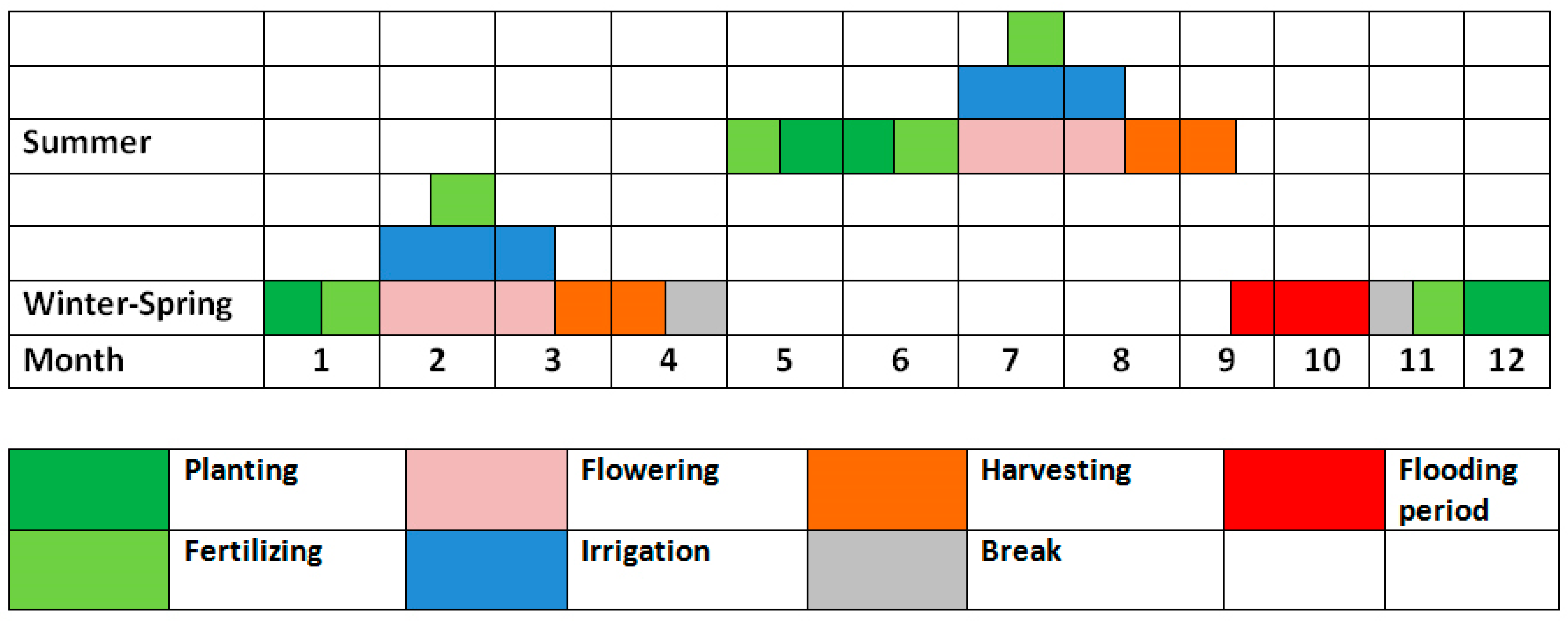
There are four climate stations, three stations outside the boundary (Khe Sanh, Hue and Nam dong stations) with the monthly data available and one station inside the boundary with the daily data from 2005 to 2013 (Aluoi station) (Figure 1). We used daily climate data (e.g., daily rainfall, maximum and minimum temperature, solar radiation, and relative humidity) for the model inputs, and monthly data for the Weather Generator (WGN) parameters. There are no hydrometric stations inside or at the outlet of the A-Luoi district. The closest hydrometric station to A-Luoi, called “Thuong Nhat,” is located east of the study area that used for parameterization in A-Luoi watershed. The FAO (Food and Agriculture Organization of the United Nations)-soil map [13] was improved based on local soil data and was also used in this study. This soil map contains information for two soil depths: in topsoil (0–30 cm) and subsoil (30–100 cm). Land use statistics in 2010 was obtained from Department of Natural Resources and Environment in Thua Thien Hue Province. The land use statistics contains different classes such as protected forest area, evergreen forests, bare lands, residential area, paddy rice lands and other agricultural lands. Forest is dominant land use in the study area and more than 90% of the area coved by evergreen forests. Rice is dominant agriculture crops and cultivated two times per year: Summer-Autumn and Winter-Spring periods (Figure 2). The surface water is the sources of irrigation/inundation for rice. Digital Elevation model (DEM) was derived from Shuttle Radar Topography Mission (SRTM) with 30m resolution. Crop schedule and yield data [14] were implemented in the model in order to simulate crop growth in SWAT. Moderate Resolution Imaging Spectroradiometer (MODIS) time series data (i.e., MOD16 product, including potential and actual evapotranspiration) were used to extract monthly evapotranspiration. These data were further used to calibrate the hydrological model.

2.3. Model Configuration

SWAT is able to predict the impact of land management practices on soil and water. Additionally, SWAT can simulate water quality and quantity as well as crop growth. The main components of the SWAT model consist of weather, hydrology, plant growth, nutrient, pesticide, bacteria and land management [1]. In this study, we focused only on the hydrologic, plant growth and land management components of the SWAT model. In SWAT, a watershed is partitioned into sub-basins using DEM, which are then further subdivided into HRUs (Hydrological Response Units) with homogenous soil, land use and slope characteristics. HRUs are the basis of water balance calculation. The water in each HRU can be stored in four levels: snow, soil profile (0–2 m), shallow aquifer (0–2 m) and deep aquifer (2–20 m). Rafiei Emam et al. [15] revealed that a single HRU could not show the characteristics of a sub-basin. Therefore, we used multiple HRUs for sub-basin analysis in this research. In SWAT, a water balance calculation is simulated in two separate components: land phase and routing phase. The land phase controls the amount of water, sediment, nutrient and pesticide loadings to the main channel in each sub-basin, while the routing phase defines the movement of water, sediment and nutrient loadings from the channel networks to the outlet. The water balance is calculated in the land phase using the following Equation (1):

$$S{W}_t=S{W}_0+{{\displaystyle \sum }}_{i=1}^t(R_{day}-Q_{surf}-E{T}_a-W_{seep}-Q_{gw}),$$

(1)

where $S{W}_t$ is the soil water content, $S{W}_0$ is the initial soil water content, $R_{day}$ is the amount of precipitation, $Q_{surf}$ indicates surface runoff, $E{T}_a$ shows actual evapotranspiration, $W_{seep}$ is the amount of percolation and $Q_{gw}$ shows the return flow.

In this study, surface runoff was simulated using a Soil Conservation Service Curve Number (SCS-CN). The runoff curve number is an empirical parameter used for predicting direct runoff or infiltration from rainfall excess. The curve number method was developed by the USDA Natural Resources Conservation Service [16]. SCS is widely used and is an efficient method for determining the approximate amount of direct runoff from a rainfall event in a particular area. It is based on the area’s hydrologic soil group, land use, treatment and hydrologic condition. Percolation was simulated with a layered storage routing technique combined with a crack flow model; and potential evapotranspiration (PET) was simulated using the Penman-Monteith method. The actual evapotranspiration was predicted based on PET in addition to soil and crop factors based on the methodology developed by Ritchie [17]. The daily value of the Leaf Area Index (LAI) was used to divide the PET into potential soil evaporation and potential plant transpiration. LAI and root development were predicted by the crop growth component of SWAT. In SWAT, soil erosion is calculated with MUSLE algorithm (Modified Universal Soil Loss Equation) [18], which is a modified version of USLE (Universal Soil Loss Equation) [19]. USLE is a function of rainfall energy, while MUSLE is a function of runoff.

To better understand the hydrological behavior, which leads to a better calibration of the model, we used an automated digital filter program [20] to separate discharge into base flow and surface runoff. Using this approach, the low-frequency base flow component was separated from high-frequency runoff components through a low-pass filter [21]. These data further were used to calibrate the hydrological model. Meaurio et al. [22] used the same method to calculate a base flow constant. More details are presented by Arnold and Allen [23]. In this research, watershed was delineated into 20 sub-basins using an SRTM map and stream network in an ArcGIS environment. The area of watershed is approximately 41,000 ha. Some 54 HRUs were created by integrating land use, soil and slope maps. Because A-Luoi is a mountainous area, we estimated precipitation (PLAPS) and temperature (TLAPS) difference by elevation. PLAPS is precipitation lapse rate (mm H₂O/km), and TLAPS refers to temperature lapse rate (°C/km). For this aim, all sub-basins with a difference in elevation greater than 100 m were selected and PLAPS and TLAPS were applied. The PLAPS and TLAPS were estimated at 243.2 mm and −5.8 °C per km using climate and elevation data. Rice is the dominant agriculture crop in A-Luoi; therefore, the crop schedule for rice was applied to the model.

2.4. Calibration, Validation and Uncertainty Analysis

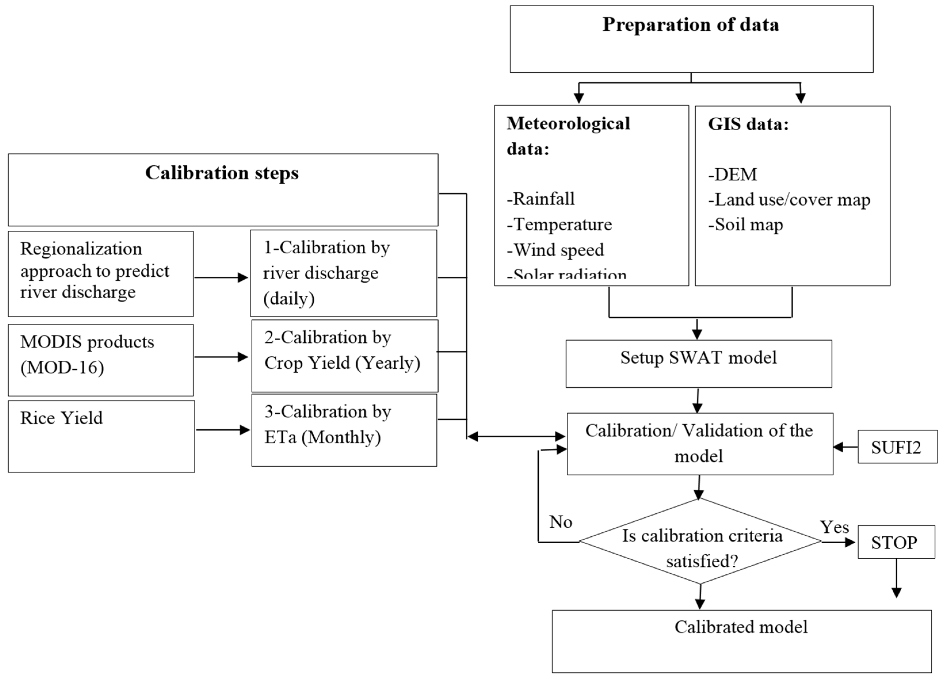
The A-Luoi district is ungauged; therefore, to calibrate the models we used different approaches. The model was calibrated and validated by the daily river discharge, yearly crop yield and monthly evapotranspiration during January 2006 and December 2010, with the three-year warm up period based on data in 2005, repeated three times. Figure 3 shows the work plan of the calibration process.

2.4.1. Regionalization Approach

The hydrological model’s parameters for ungauged basins (i.e., without any river discharge measurements) can be predicted using the regionalization method [24,25]. Usually watersheds with similar characteristics show similar hydrological treatments and therefore the hydrological parameters can be transferred from the same watersheds. This transformation is called regionalization. A number of basin characteristics (e.g., soil, topography, land use, precipitation, and temperature) were presented in Samaniego and Bardossy [26]. There are different methods for this transformation including regression methods [27], spatial proximity [28] and physical similarity [29]. Parajka et al. [30] used geostatistical methods (i.e., Kriging) to transfer model parameters. Sun et al. [31] used a new approach to calibrate hydrological parameters in ungauged basins. They used the river water level obtained from satellite radar altimetry observations at the outlet of the basin instead of river discharge. In another work, Sun et al. [32] used the river flow width obtained through satellite observation as a surrogate for river discharge records to calibrate a hydrological model.

Because there is not a river discharge station at the outlet of our study area and we cannot calibrate the relevant parameters directly, we used regionalization approach to transfer the relevant parameters from the nearby catchment to our study area. To do that, Thuong Nhat catchment, 45 km away from the center of A-Luoi, with the observed discharge data was selected. Data is available at daily scale from 2005 to 2010 at Nhat station in this catchment. The characteristics of the two basins are similar with difference annual precipitation of 2.6%. More physical characteristics are presented in

Table 1. Properties of the donor and target catchments.

Catchment	Climate Station	River	Rain Gauge Station	Rainfall (Annual) mm	Area Km2	Slope (Mean) %	Elevation (Mean) m	Land- Use *	Soil *	L/W **
A-Luoi	Aluoi	Song Sia River	Aluoi	3900	408	38	495	Forest	Orthic Acrisols	1.90
Thuong Nhat	Nam Dong	Ta Trach River	Nam Dong	3800	125	42	490	Forest	Orthic Acrisols	1.05

* Dominant landuse and soil type are mentioned; ** L/W: Length/Width of catchment.

.

We set up a new model in this basin and the model was calibrated based on the river discharge data. The calibrated parameters were further transferred into our original model of A-Luoi basin. The SUFI-2 algorithm (Sequential Uncertainty Fitting, ver. 2) [33] in the SWAT-CUP package was used to calibrate and analyze uncertainty. Nash-Sutcliffe coefficient (Equation (2)) was computed as the objective function for river discharge in a gauged basin:

$$NSE=1-\frac{{{\displaystyle \sum }}_{i=1}^n{\left(Q_{obs}-Q_{sim}\right)}^2}{{{\displaystyle \sum }}_{i=1}^n{(Q_{obs}-{\overline{Q}}_{obs})}^2}$$

(2)

where $Q_{obs}$ and $Q_{sim}$ are the measured and simulated data, respectively, n is the total number of data records and ${\overline{Q}}_{obs}$ is the mean measured data.

In SUFI-2 all sources of uncertainty (e.g., uncertainty in input data, conceptual model and parameters) are represented in model output. The degree of uncertainty is measured by two factors: P-factor, which represents the percentage of measured data bracketed by 95% prediction uncertainty (95PPU), and R-factor, which is the ratio of average width of 95PPU to standard deviation of measured data. The model attempts to bracket most of the data (P-factor = 1) within a narrow band (R-factor = 0). However, often a balance must be reached between these two factors.

2.4.2. Calibration Based on Crop Yield

We calibrated a crop yield because calibration using a crop yield gives more confidence on actual evapotranspiration, and hence give the precise estimation of other water components such as, soil moisture, surface runoff and percolation [15]. The SUFI-2 algorithm was used to calibrate the crop parameters and uncertainty analysis. A mean square error was used as the objective function. There are several parameters that affect crop yield. These parameters include the heat unit (HU), harvest index (HI), and bio target (BIO-TARG). The HU is the amount of heat that brings plants to maturity, the HI is the fraction of above-ground dry biomass to yield crops, and the BIO-TARG is the potential plant yield. We optimized these parameters in order to calibrate crop yield in our hydrological model.

Plant growth in the model is usually inhibited by temperature, water, nitrogen and phosphorous stress factors. Rafiei Emam et al. [34] evaluated the water and temperature stresses of winter wheat using a climate change model. Temperature is a very important factor for plant growth; plants can grow only if the mean temperature exceeds the base temperature of plant. The accumulation of daily mean air temperatures above the plant’s optimum temperature over the plant-growth period is called a heat unit. The base (or optimum) temperature varies for different plants, for instance, paddy rice has base temperature of 10 °C.

2.4.3. Calibration Based on ETa Using MODIS Products

Because agriculture covers only a small part of A-Luoi and most of the lands in the study area are covered by forest, we used ETa products of MODIS in order to calibrate the SWAT model. There have been several attempts to use satellite observation of evapotranspiration to calibrate a hydrological model. Immerzeel and Droogers, [35] used MODIS satellite images to calibrate the hydrological model using evapotranspiration data. Cheema et al. [36] calibrated the SWAT model in the irrigated Indus basin based on spatially distributed ET derived from remotely sensed data.

Nash-Sutcliff efficiency (NSE) and coefficient of determination were used to assess the SWAT model based on ETa calibration. NSE was used as the objective function to compare the monthly observed and simulated ETa.

We used MOD16 products [37] of MODIS from 2006 to 2013 on a monthly scale. We downloaded 90 images (6 images are missing) in Central Vietnam (h = 28 and v = 7). We further extracted PET and ETa of MOD16 products in ArcGIS environment in our study area and summarized data in each sub-basin. We analyzed the reliability of the data and finally these data were used to calibrate the SWAT hydrologic model.

3. Results and Discussion

3.1. Regionalization Outcome

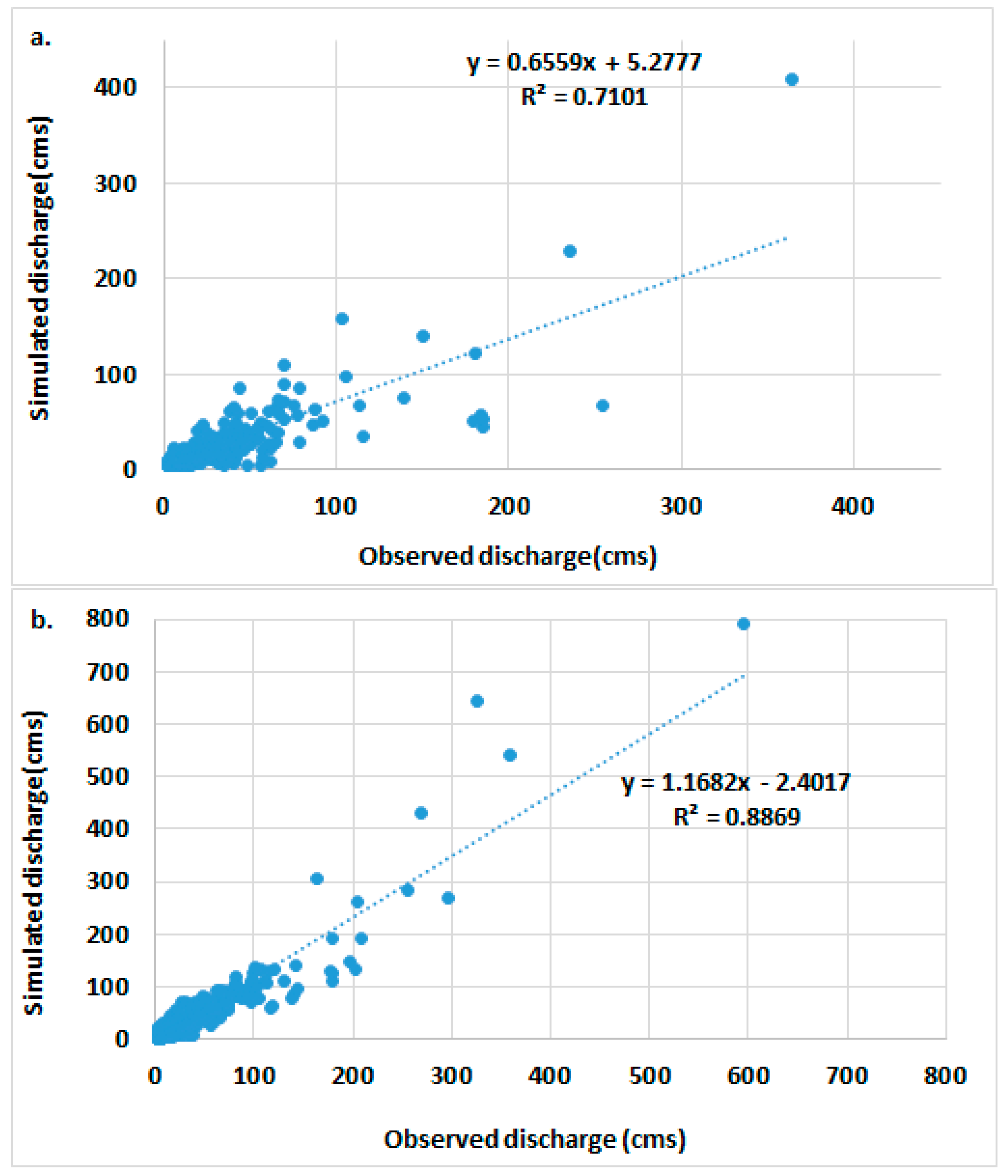
The results of calibration and validation of Nam Dong watershed, a nearby watershed to A-Luoi, showed a good performance of the model with high NS (0.74, 0.51) and R² (0.71, 0.88) both for calibration and validation, respectively. The sensitivity analysis shows that the curve number (CN) is the most sensitive parameter followed by Base Flow Alpha Factor for Bank Storage (Alpha-BNK) and effective hydraulic conductivity in the main channel (CH-K2). The importance of these parameters has been reported by some other researchers. Rafiei Emam et al. [2,38] mentioned that CN is the most sensitive parameter in mountainous area. Luo et al. [39] revealed that the parameters of CH-K2 and Alpha-BNK play important roles in the calibration of the SWAT model in Tropical areas.

Comparing observed with simulated discharge shows that there is a good agreement between the simulated daily stream flow and the observed data. Additionally, the scatter plot between observed and simulated data for both calibration and validation show the pretty high performance of the model (Figure 4). Therefore, the calibrated parameters were transferred into the A-Luoi model for further processing.

3.2. Parameterization for Crop Yield

The sub-basins with paddy rice cultivations (i.e., sub-basins located south of the A-Luoi area) were selected for the parameterization of the model based on crop yield. The calibration based on crop makes the model results more confident [15]. There is a direct relationship between crop yield and evapotranspiration; therefore, the calibration of the model based on yield improves the simulation of other water components.

The sensitivity analysis showed that all crop parameters (e.g., HEAT-UNIT, BIO-TARG, HI) were sensitive to crop yield. Figure 5 shows the results of calibration and validation of the paddy rice yield. As illustrated, observed yields are inside or quite close to simulated yield band, indicating good results. The yield varies between 26.5 and 30 ton/ha, with the highest yield found in the year 2010. The RMSE for yield was 2.1 kg·ha⁻¹ and 2.39 kg·ha⁻¹ in the calibration and validation period, respectively, which shows pretty good accuracy of calibration. Akhavan et al. [40] revealed the high range of RMSE from 80 to 4220 kg·ha⁻¹ for calibration and validation of wheat yield in Hamedan, Iran. They mentioned that the large RMSE could be due to the lack of data concerning management practices, which can be accounted in our study area as well. The P-factor is quite good, with a value larger than 0.8 for calibration and 0.89 for the validation period. The large R-factor (i.e., R-factor = 3) represents a large uncertainty. The reason for this amount of uncertainty is probably due to low data availability and insufficient accounting for agriculture and industrial water use in the model. The other reason is due to Nitrogen (N) stress, because the N is removed from the farmlands quickly by rising rainfall and surface runoff.

3.3. Parameterization for ETa Based on MODIS ET Time Series

3.3.1. Reliability of MODIS Data

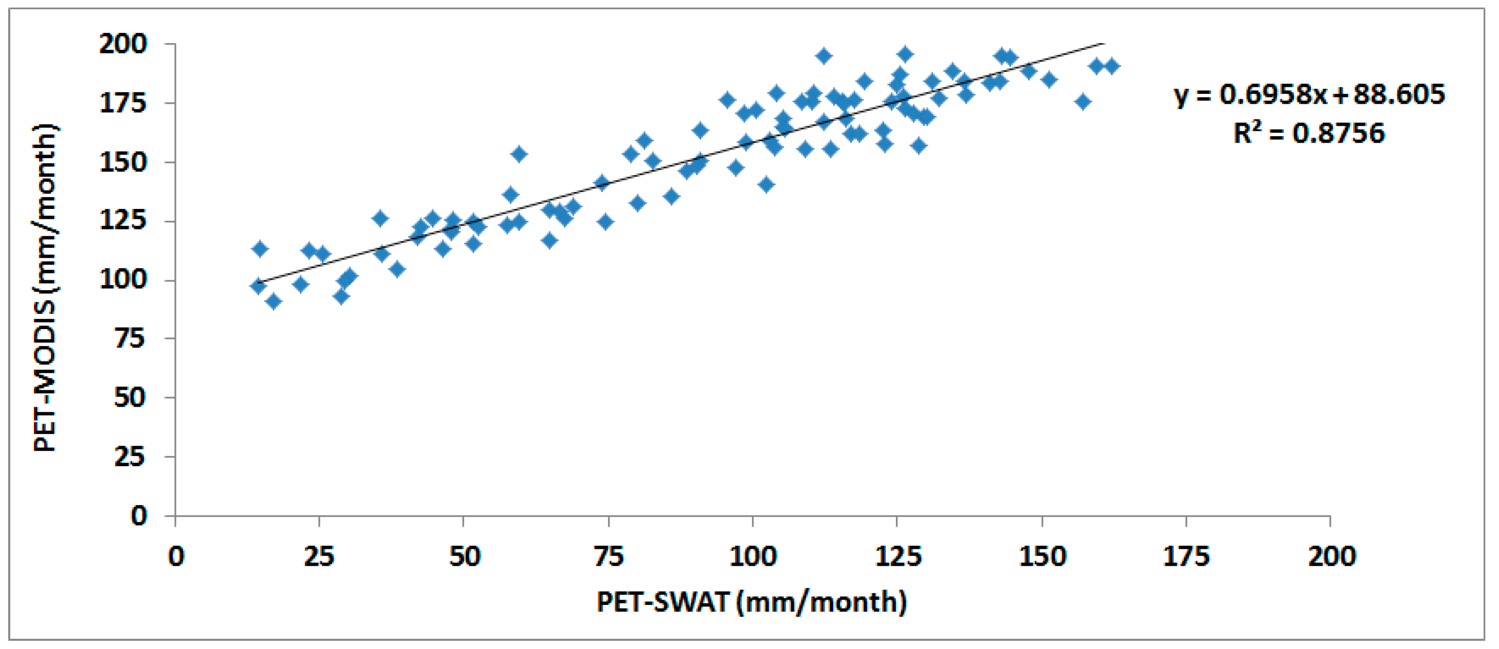
To calibrate the model based on the evapotranspiration, first we evaluated the reliability of the MOD16 of MODIS time series data. Toward this aim, the PET of MOD16 was extracted monthly from January 2006 to December 2013. The average PET-MODIS in the basin was plotted against PET calculated by measuring data in the SWAT model using the Penman-Monteith method (Figure 6). As Figure 6 shows, there is a high correlation between PET of MOD16 and PET calculated by SWAT. The dynamics of time series of SWAT and PET-MODIS was mapped in Figure 7. The dynamics of PET of SWAT and MODIS are very similar to each other, but there is a bias between these data. The amount of PET in winter, when there is less precipitation, is more reliable than the other months. The peak of PET-MODIS in summer, May to August, is higher than measured data (approximately 10 to 70 percent more than measured one), which makes it unreliable in these months. Therefore, we calculated the bias between two data time series. Toward this aim, we divided the year into two periods: first from October to March and second from April to September. Then we analyzed data based on rational analysis and found two constants for these two periods. To correct the bias, for the first period, the PET data was multiplied by 0.45, and for second period, the PET data was multiplied by 0.70. Then, the corrected PET of MODIS (PETm_c) multiplied to the ratio of PET/ETa ($\rho$) of MODIS in order to bias correction of ETa.

$$\rho =\frac{ETPm}{ETam}$$

(3)

$$ETa{m}_c=ETP{m}_c\times \rho$$

(4)

where PETm is the potential evapotranspiration of MODIS, ETam is the actual evapotranspiration extracted from MODIS, ETam_c is the bias corrected of ETa-MODIS, and PETm_c is the bias corrected PET-MODIS results.

3.3.2. Procedure of Model Calibration Using ET-MODIS

In this step, the SWAT Model was calibrated in the sub-basins with dominant forest cover. To calibrate the SWAT model by ETa data, first we kept the calibrated parameters for river discharge and crop yield and then we chose the parameters that affected ETa (

Table 2. Soil and Water Assessment Tools (SWAT) parameters and their initial and final range for river discharge, evapotranpiration (ETa) and crop yield calibration.

ID	Parameters *	Description	Initial Range	Final Range	Additional Information
1	r__CN2.mgt	Curve number	−0.5 to 0.5	−0.150 to 0.25	Parameters of river discharge
2	r__SOL_BD().sol	Soil bulk density	−0.5 to 0.5	−0.11 to 0.72
3	r__SOL_K().sol	Soil conductivity (mm/h)	−0.5 to 0.5	−0.68 to 0.99
4	r__SOL_AWC().sol	Soil available water storage capacity (mm H2O/mm soil)	−0.5 to 0.5	0.07 to 0.50
5	v__CH_K2.rte	Effective hydraulic conductivity in main channel	50 to 400	302 to 394
6	v__ALPHA_BNK.rte	Base flow alpha factor for bank storage	0 to 1	0.1 to 0.7
7	r__CH_N2.rte	Manning value for main channel	−0.5 to 0.5	−0.39 to 0.20
8	r__OV_N.hru	Manning value for overland channel	−0.5 to 0.5	−0.15 to 0.42
9	r__SLSUBBSN.hru	Average slope length (m)	0.5 to 0.5	0.46 to 0.90
10	v__GWQMN.gw	Threshold water level in shallow aquifer for base flow	100 to 5000	1250 to 3600
11	v__GW_DELAY.gw	Ground water delay time (days)	10 to 500	227 to 400
12	v__ALPHA_BF.gw	Base flow alpha factor (days)	0.04 to 0.07	0.040 to 0.075
13	v__GW_REVAP.gw	Revap coefficient	0.02 to 0.2	0.0.03 to 0.15
14	v__REVAPMN.gw	Threshold water level in shallow aquifer	0 to 500	100 to 250
15	v__ESCO.hru	Soil evaporation compensation factor	0.1 to 1.0	0.40 to 0.65
16	v__WAVP{8}.plant.dat	Rate of decline in radiation use efficiency per unit increase in vapor pressure deficit.	1 to 50	43 to 46	Parameters of ETa
17	V__DLAI{8}.plant.dat_____FRST	Fraction of growing season when leaf area begins to decline in forest area	0.15 to 1	0.95 to 0.99
18	V__BLAI{8}.plant.dat_____FRST	Maximum potential leaf area index of forest areas	2 to 10	2.7 to 5.7
19	v__HEAT_UNITS{[],1}.mgt____FRST	Total heat units for plant to reach maturity in forest areas	1000 to 4500	2900 to 3350
20	v__HEAT_UNITS{[],1}.mgt____RICE	Total heat units for plant to reach maturity in paddy areas	1000 to 4500	4000 to 4600	Parameters of crop
21	v__HI{[],1}.mgt	harvest index	0.6 to 0.99	0.9 to 0.99
22	v__BIO-TARG.mgt	bio target	10 to 50	35 to 50

* r parameter value is multiplied by 1 + given value, v parameter value is replaced by a value from the given range.

). Five parameters were used for sensitivity analysis using a one-at-a-time method [33].

The results of the global sensitivity analysis are shown by p-value and t-test, which show the measure of sensitivity and the significance of sensitivity, respectively. The results show that BLAI (t-test = [2.5], p-value = 0.05) is the most sensitive parameter for ET calibration followed by DLAI (t-test = [1.5], p-value = 0.3) and ESCO (t-test = [0.6], p-value = 0.5). BLAI represent the maximum potential leaf area index of trees. BLAI is one of the six parameters used to determine leaf area development of plants during the growing season. DLAI is the “fraction of the growing season when the leaf area begins to decline” [41]. ESCO depends on soil characteristics and controls the soil evaporation.

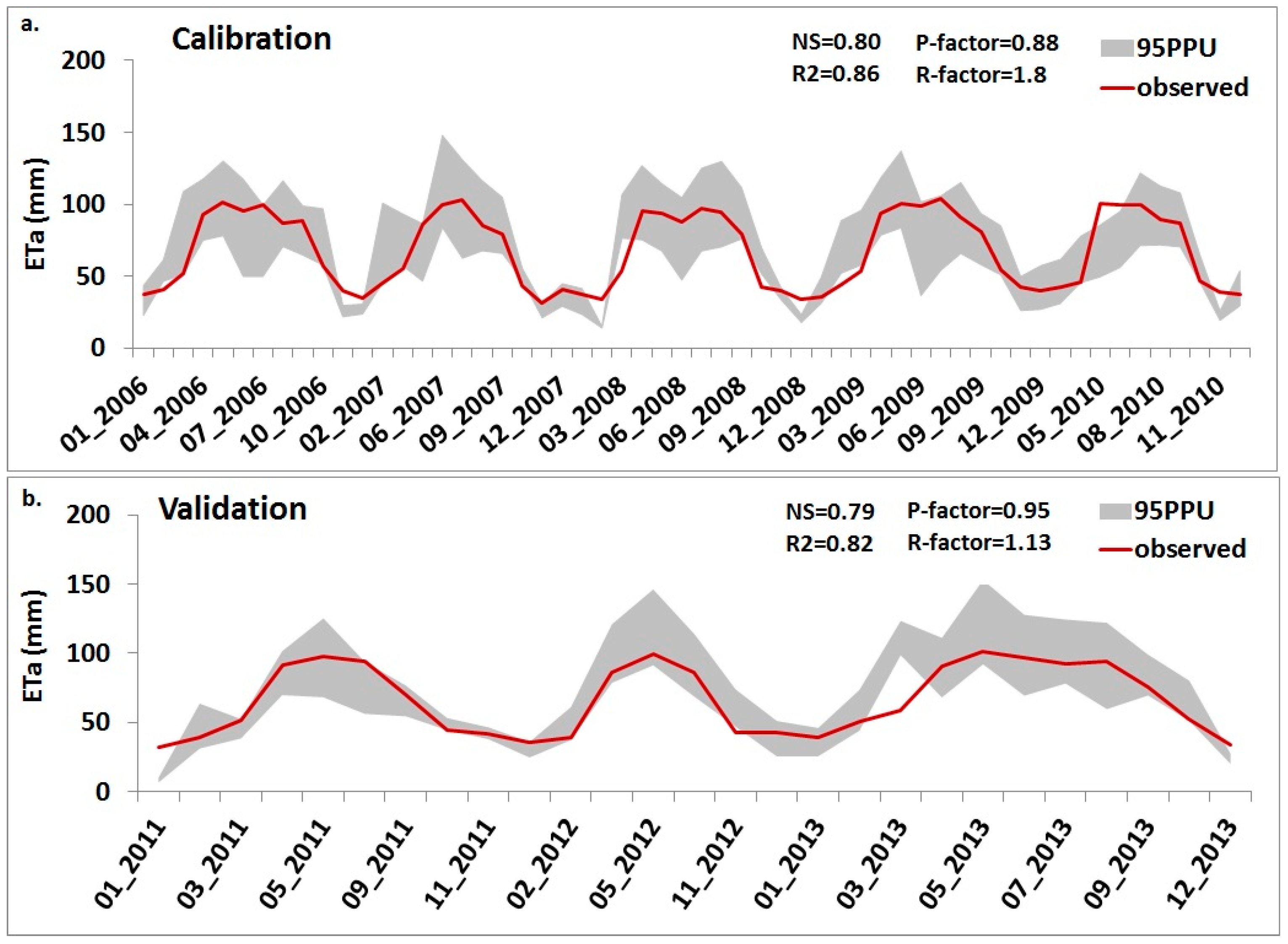
The results of the model calibration were satisfactory. Figure 8a shows the results of the ETa calibration in the forest areaof watershed. As Figure 8 depicts, the observed data are captured by the predicted band (95PPU). In all of the sub-basins, the temporal changes of ETa were simulated quite well, with a Nash-Sutcliffe (NS) and coefficient of determination (R²) higher than 0.79. Moriasi et al. [42] and Santhi et al. [43] reported that if the NS and R² are greater than 0.5, then the performance of the model is satisfactory. The results also show that the simulated ETa has variation in different seasons. Petković et al. [44] mentioned that relative humidity and a wind speed of two meters are two factors that play a role in the variation of ET. The same results were also presented by Nguyen and Kappas [3]. As Figure 8a,b shows, the lowest evapotranspiration is from November to February, when the average temperatures are lower than over the other months.

3.4. Quantification of Water Components

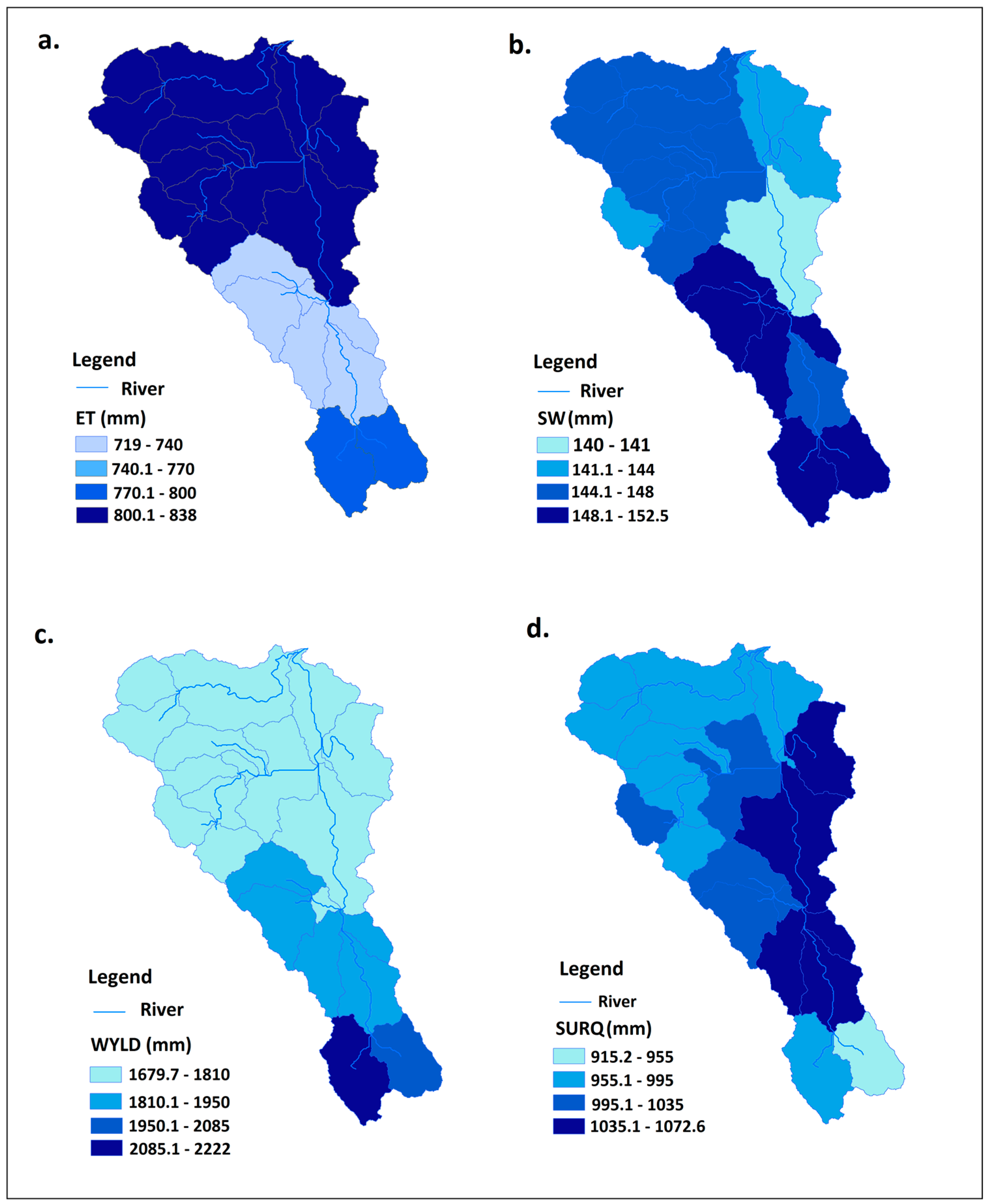
After the model was calibrated by river discharge, crop yield and ET, we computed the water resource availability in the watershed. Figure 9 shows the water resources availability including the monthly (for the time period 2006 to 2013) water yield (i.e., the net amount of water that leaves the sub-basin and contributes to streamflow in the reach during the time period), green water resources (i.e., soil water content) and green water flow (i.e., actual evapotranspiration) in the A-Luoi watershed of Vietnam.

There is a significant spatial variation in the hydrological components across the watershed. The distributed maps showed that in the north of basin, where the rainfall and water yield are small, and actual evapotranspiration (ETa) is high. The ETa shows the amount of water that is consumed by plants. The annual average ETa (M95PPU) during the period of 2006 to 2013 varied from 719 mm/year to 838 mm/year in different parts of the watershed. The lowest amount of ETa was found in the southern area, while the northern area had the highest ETa (Figure 9a). The soil water content map (Figure 9b) shows the area where rain-fed Rubber and other perennial crops have a better chance of high production due to soil moisture. The southern area has the highest soil moisture, while the eastern area has the lowest soil moisture. This is probably due to soil characteristics in different parts of the watershed. Water yields (Figure 9c) varied from 1679 mm/year to 2222 mm/year in different sub-basins from 2006 to 2013. Water yield is the net amount of water that leaves the sub-basin and contributes to streamflow in the reach during the time period.

The annual average rainfall from 2006 to 2013 was 4049 mm/year. We calculated the monthly average water components in the entire basin. The results of average monthly evapotranspiration showed that ETa is highest in May, due to the high demand of water by forests and plants in this month. The prediction uncertainty in summer is higher than in winter due to the high consumption of water by plants during these months (Figure 10a). Paddy rice lands affect the ETa considerably. The total ratio of ETa to rainfall for eight years (2006–2013) was calculated at 36%, showing that the ETa is always less than rainfall in tropical areas. Nevertheless, this ratio is lowest in October and highest in January.

3.5. Surface Runoff

The result of the SWAT hydrological model shows that the surface runoff is high in upstream areas of basins. Vegetation cover, soil type and slope gradient [45] are the important factors affecting surface runoff. Land use change and deforestation lead to increasing surface runoff and hence soil erosion. The results showed that the spatial average of surface runoff in the watershed varied from 915 mm/year to 1072 mm/year from 2006 to 2013. The area upstream has the highest amount of surface runoff probably due to its high slope.

The monthly average 95PPU of surface runoff was extracted in order to understand the temporal distribution and uncertainty of surface runoff (Figure 10b). This figure reveals that October has the highest surface runoff, with an average of approximately 368 mm/month. The surface runoff during September to November has the highest uncertainty, probably due to a conceptual model and parameter uncertainties. However, all uncertainties are depicted in the 95PPU band, shown in gray in the figure. As the Figure 10b shows, there is a strong relationship between surface runoff and rainfall. In February, the rainfall is the lowest and the uncertainty surface runoff prediction is also low, while in October, the month with the highest rainfall, the uncertainty is high. Surface runoff mainly occurred in areas with a slope higher than 25%. This slope class includes the farmlands, which have a surface runoff larger than forest land use. Nevertheless, the surface runoff in the paddy rice lands is low because the slopes in this area usually break down by terracing, therefore, the time concentration is increased. The soil erosion and sedimentation followed the surface runoff behavior [5]. Therefore, with an increase in surface runoff, the soil erosion and hence sedimentation is increased. The same results were presented by Phuong et al. [5]. The results revealed that surface runoff is highest when the amount of rainfall reaches the maximum amount during the year.

3.6. Best Management Practices (BMPs)

BMPs are conservation programs that minimize pasture and agricultural runoff and nutrient loads. Many researchers use BMPs to conserve agricultural and pastoral lands. For example, the effects of two BMP systems on water quality in a livestock pasture were discussed by Sheshukov et al. [46]. Smith et al. [47] presented BMPs to conserve agricultural lands. Arabi et al. [48] used four BMPs types in different land use classes in order to reduce sediment and nutrients loads in the watershed.

The southern part of the A-Luoi basin has the highest runoff and hence flooding, which probably resulted in soil erosion and sedimentation in this area. We installed two types of BMPs structures—terracing and contouring—in agricultural lands with slope higher than 25% in early 2005. A terrace was designed in the field to decrease runoff and protect the land against erosion. It is constructed across a slope on a contour. Terracing in the SWAT model is simulated by adjusting runoff and erosion parameters such as the USLE practice factor, the slope length and curve number. A contouring system simulates a contour to the HRU on a specified day. Contour planting is the method of planting crops in straight rows in small ridges. It results in increased roughness and soil storage. Similar to terracing, contouring is simulated by adjusting the USLE practice factor and curve number. All parameters were adjusted based on the land slope suggested by SWAT documents and literature [5].

The results revealed that terracing in dry agricultural lands resulted in a reducing surface runoff and sediment yield of approximately 33% and 58%, respectively, whereas increasing ETa only increased approximately 35%. The amount of soil water content also increased 136% from 2006 to 2013. Nevertheless, implementing contouring has more significant impact than terracing in farmlands with a slope of more than 25% (

Table 3. The average water components (2006–2013) in Hydrological Response Units (HRUs) in dry farmlands with slope larger than 25%.

BMP	Surface Runoff (mm)	Percolation (mm)	Soil Water Content (mm)	ETa (mm)
No application	150	1.5	11	28
Terracing	100.5	24	26	38
Contouring	75	41	37	44

). The BMPs reduce surface runoff and sedimentation, whereas percolation, soil moisture and ETa decrease. Labrière et al. [7] mentioned that land use with good management practices protect lands against soil erosion. They concluded that implementations such as contour planting, no-till farming and a vegetative buffer strip can decrease soil erosion by up to 99%.

4. Conclusions

A hydrological model based on SWAT was implemented in the A-Luoi district in the Central Vietnam in order to assess water and land resource management. A multi-calibration procedure that takes into account not only the stream flow but also the actual evapotranspiration and crop yield was investigated. We used the regionalization approach in the ungauged basin of A-Luoi to transfer the parameters from the nearby calibrated watershed in our model. The model was well calibrated based on various observed data (e.g., river discharge, actual evapotranspiration and crop yield). The results showed that BMPs implementation in farmlands could help to reduce the surface runoff and hence soil erosion and sedimentation.

One of the difficulties to calibrate the model is that some of the parameters might be sensitive to more than one objective, we overcome this problem by choosing the best range of the parameter’s value instead of an absolute value in each step of the calibration.

Our results showed that the ETa product of MODIS can be used for the calibration of the hydrological model in case of data scarcity. However, it is important to note that bias correction should apply to this product before using it in the calibration process.

Based on the results, surface runoff was high, probably due to the geometry of the basin and its soil properties. The surface runoff is high, which leads to rising soil erosion and sedimentation. Our results show that using BMPs leads to decreased surface runoff and hence soil erosion in agricultural lands. Therefore, we suggest implementing terracing/contouring systems in the steep farmlands of the A-Luoi area.

References

1. Arnold, J.G.; Srinivasan, R.; Muttiah, R.S.; Williams, J.R. Large area hydrologic modeling and assessment—Part 1, model development. J. Am. Water Resour. Assoc. 1998, 34, 73–89. [Google Scholar] [CrossRef]
2. Rafiei Emam, A.; Kappas, M.; Abbaspour, K.C. Simulation of water balance components in a watershed located in central drainage basin of Iran. In Remote Sensing of the Terrestrial Water Cycle, Geophysical Monograph 206; Lakshmi, V., Ed.; American Geophysical Union: Washington, DC, USA; Wiley & Sons Press: New York, NY, USA, 2015; pp. 463–478. [Google Scholar]
3. Nguyen, H.Q.; Kappas, M. Modeling Surface Runoff and Evapotranspiration using SWAT and BEACH for a Tropical Watershed in North Vietnam, Compared to MODIS Products. Int. J. Adv. Remote Sens. GIS 2015, 4, 1367–1384. [Google Scholar]
4. Schuol, J.; Abbaspour, K.C.; Yang, H.; Srinivasan, R.; Zehnder, A.J.B. Modeling blue and green water availability in Africa. Water Resour. Res. 2008, 44, 1–18. [Google Scholar] [CrossRef]
5. Phuong, T.T.; Thong, C.V.T.; Ngoc, N.B.; Chuong, H.V. Modeling Soil Erosion within Small Moutainous Watershed in Central Vietnam Using GIS and SWAT. Resour. Environ. 2014, 4, 139–147. [Google Scholar]
6. Qiao, L.; Herrmann, R.B.; Pan, Z. Parameter Uncertainty Reduction for SWAT Using Grace, Streamflow, and Groundwater Table Data for Lower Missouri River Basin. J. Am. Water Resour. Assoc. 2013, 49, 343–358. [Google Scholar] [CrossRef]
7. Labrière, N.; Locatelli, B.; Laumonier, Y.; Freycon, V.; Bernoux, M. Soil erosion in the humid tropics: A systematic quantitative review. Agric. Ecosyst. Environ. 2015, 203, 127–139. [Google Scholar] [CrossRef] [Green Version]
8. Cerdà, A. Effect of climate on surface flow along a climatological gradient. A field rainfall simulation approach. J. Arid Environ. 1998, 38, 145–159. [Google Scholar] [CrossRef]
9. Xu, X.Y.; Yang, H.B.; Yang, D.W.; Ma, H. Assessing the impact of climate variability and human activities on annual runoff in the Luan River basin, China. Hydrol. Res. 2013, 44, 940–952. [Google Scholar] [CrossRef]
10. Nguyen, A.H. Comprehensively Studying Geographical Arising and Land Degradation Aiming the Purpose of Reasonably Using Land Resource and Preventing Disaster in Binh-Tri-Thien Region. Ph.D. Thesis, University of Mining and Geology, Hanoi, Vietnam, 2010. [Google Scholar]
11. Phuong, T.T.; Chuong, H.V. Simulating effects of land use change on soil erosion in Bo River basin in the Central of Vietnam. J. Agric. Rural Dev. 2013, 2. [Google Scholar]
12. Soil Survey Staff. Keys to Soil Taxonomy, 12th ed.USDA-Natural Resources Conservation Service: Washington, DC, USA, 2014.
13. Food and Agriculture Organization of the United Nations (FAO). The Digital Soil Map of the World and Derived Soil Properties; Version 3.6; FAO: Rome, Italy, 2003. [Google Scholar]
14. Master Plan of Aluoi 2015, District, Development, and Investment Plan (DDIP); Aluoi district Authority: Aluoi, Vietnam.
15. Rafiei Emam, A.; Kappas, M.; Akhavan, S.; Hosseini, S.Z.; Abbaspour, K.C. Estimation of groundwater recharge and its relation to land degradation: Case study of a semi-arid river basin in Iran. Environ. Earth Sci. J. 2015, 74, 6791–6803. [Google Scholar] [CrossRef]
16. USDA: United States Department of Agriculture. Urban Hydrology for Small Watersheds, Technical Release 55 (TR-55), 2nd ed.Natural Resources Conservation Service, Conservation Engineering Division: Washington, DC, USA, 1986.
17. Ritchie, J.T. A model for predicting evaporation from a row crop with incomplete cover. Water Resour. Res. 1972, 8, 1204–1213. [Google Scholar] [CrossRef]
18. Williams, J.R. Sediment Yield Prediction with Universal Equation Using Runoff Energy Factor; Agricultural Research Service: Washington, DC, USA, 1975; Volume ARS-S-40.
19. Wischmeier, W.H.; Smith, D.D. Predicting Rainfall-Erosion Losses from Cropland East of the Rocky Mountains. Agriculture Handbook; U.S. Department Agriculture: Washington, DC, USA, 1965; p. 282.
20. Arnold, J.G.; Allen, P.M. Automated methods for estimating base flow and ground water recharge from streamflow records. J. Am. Water Resour. Assoc. 1999, 35, 411–424. [Google Scholar] [CrossRef]
21. Stewart, M.; Cimino, J.; Ross, M. Calibration of Base Flow Separation Methods with Streamflow Conductivity. Ground Water 2007, 45, 17–27. [Google Scholar] [CrossRef] [PubMed]
22. Meaurio, M.; Zabaleta, A.; Uriarte, J.A.; Srinivasan, R.; Antigüedad, I. Evaluation of SWAT models performance to simulate streamflow spatial origin. The case of a small forested watershed. J. Hydrol. 2015, 525, 326–334. [Google Scholar] [CrossRef]
23. Arnold, J.G.; Allen, P.M. Estimating hydrologic budgets for three Illinois watersheds. J. Hydrol. 1996, 176, 57–77. [Google Scholar] [CrossRef]
24. Vandewiele, G.L.; Atlabachew, E. Monthly water balance of ungauged catchments obtained by geographical regionalization. J. Hydrol. 1995, 170, 277–291. [Google Scholar] [CrossRef]
25. Bárdossy, A. Calibration of hydrological model parameters for ungauged catchments. Hydrol. Earth Syst. Sci. 2007, 11, 703–710. [Google Scholar] [CrossRef]
26. Samaniego, L.; Bárdossy, A. Robust parametric models of runoff characteristics at the mesoscale. J. Hydrol. 2005, 303, 136–151. [Google Scholar] [CrossRef]
27. Bastola, S.; Ishidaira, H.; Takeuchi, K. Regionalization of hydrological model parameters under parameter uncertainty: A case study involving TOPMODEL and basins across the globe. J. Hydrol. 2008, 357, 188–206. [Google Scholar] [CrossRef]
28. Merz, R.; Blöschla, G. Regionalisation of catchment model parameters. J. Hydrol. 2004, 287, 95–123. [Google Scholar] [CrossRef]
29. McIntyre, N.; Lee, H.; Wheater, H.; Young, A.; Wagener, T. Ensemble predictions of runoff in ungauged catchments. Water Resour. Res. 2005, 41, W12434. [Google Scholar] [CrossRef]
30. Parajka, J.; Merz, R.; Bloschl, G. A comparison of regionalization methods for catchment model parameters. Hydrol. Earth Syst. Sci. 2005, 9, 157–171. [Google Scholar] [CrossRef]
31. Sun, W.C.; Ishidaira, H.; Bastola, S. Calibration of hydrological models in ungauged basins based on satellite radar altimetry observations of river water level. Hydrol. Process. 2014, 26, 3524–3537. [Google Scholar] [CrossRef]
32. Sun, W.C.; Ishidaira, H.; Bastola, S. Towards improving river discharge estimation in ungauged basins: calibration of rainfall-runoff models based on satellite observations of river flow width at basin outlet. Hydrol. Earth Syst. Sci. 2010, 14, 2011–2022. [Google Scholar] [CrossRef]
33. Abbaspour, K.C. SWAT-CUP: SWAT Calibration and Uncertainty Programs—A User Manual; Swiss Federal Institute of Aquatic Science and Technology: Dubendorf, Switzerland, 2015. [Google Scholar]
34. Rafiei Emam, A.; Kappas, M.; Hosseini, S.Z. Assessing the impact of climate change on water resources, crop production and land degradation in a semi-arid river basin. Hydrol. Res. 2015, 46, 854–870. [Google Scholar]
35. Immerzeel, W.W.; Droogers, P. Calibration of a distributed hydrological model based on satellite evapotranspiration. J. Hydrol. 2008, 349, 411–424. [Google Scholar] [CrossRef]
36. Cheema, M.J.M.; Immerzeel, W.W.; Bastiaanssen, W. Spatial quantification of groundwater abstraction in the irrigated Indus basin. Groundwater 2014, 52, 25–36. [Google Scholar] [CrossRef] [PubMed]
37. Mu, Q.; Zhao, M.; Running, S.W. Improvements to a MODIS Global Terrestrial Evapotranspiration Algorithm. Remote Sens. Environ. 2011, 115, 1781–1800. [Google Scholar] [CrossRef]
38. Rafiei Emam, A.; Mishra, B.; Kumar, P.; Masago, Y.; Fukushi, K. Impact Assessment of Climate and Land-Use Changes on Flooding Behaviour in the Upper Ciliwung River, Jakarta, Indonesia. Water 2016, 8, 559. [Google Scholar] [CrossRef]
39. Luo, Y.; Arnold, J.; Allen, P.; Chen, X. Base flow simulation using SWAT model in an inland river basin in Tianshan Mountains, Northwest China. Hydrol. Earth Syst. Sci. 2012, 16, 1259–1267. [Google Scholar] [CrossRef] [Green Version]
40. Akhavan, S.; Abedi-Koupai, J.; Mousavi, S.F.; Afyuni, M.; Eslamian, S.S.; Abbaspour, K.C. Application of SWAT model to investigate nitrate leaching in Hamadan–Bahar Watershed, Iran. Agric. Ecosyst. Environ. J. 2010, 139, 675–688. [Google Scholar] [CrossRef]
41. Arnold, J.G.; Kiniry, J.R.; Srinivasan, R.; Williams, J.R.; Naney, E.B.; Neitsch, S.L. Soil and Water Assessment Tool. Input/Output Documentation, Version 2012, TWRI TR-439; Texas Water Resources Institute, College Station: Texas, TX, USA, 2012. [Google Scholar]
42. Moriasi, D.N.; Arnold, J.G.; Van Liew, M.W.; Bringer, R.L.; Harmel, R.D.; Veith, T.L. Model evaluation guidelines for systematic quantification of accuracy in watershed simulations. Am. Soc. Agric. Biol. Eng. 2007, 50, 885–900. [Google Scholar]
43. Santhi, C.; Arnold, J.G.; Williams, J.R.; Dugas, W.A.; Srinivasan, R.; Hauck, L.M. Validation of the SWAT model on a large river basin with point and nonpoint sources. J. Am. Water Resour. Assoc. 2001, 37, 1169–1188. [Google Scholar] [CrossRef]
44. Petković, D.; Gocic, M.; Trajkovic, S.; Shamshirband, S.; Motamedi, S.; Hashim, R.; Bonakdari, H. Determination of the Most Influential Weather Parameters on Reference Evapotranspiration by Adaptive Neuro-Fuzzy Methodology. Comput. Electron. Agric. 2015, 114, 277–284. [Google Scholar] [CrossRef]
45. El Kateb, H.; Zhang, H.; Zhang, P.; Mosandl, R. Soil erosion and surface runoff on different vegetation covers and slope gradients: A field experiment in Southern Shaanxi Province, China. CATENA 2013, 105, 1–10. [Google Scholar] [CrossRef]
46. Sheshukov, A.Y.; Douglas-Mankin, K.R.; Sinnathamby, S.; Daggupati, P. Pasture BMP effectiveness using an HRU-based subarea approach in SWAT. J. Environ. Manag. 2016, 166, 276–284. [Google Scholar] [CrossRef] [PubMed]
47. Smith, C.M.; Nejadhashemi, A.P.; Leatherman, J.C. Using a BMP Auction as a Tool for the Implementation of Conservation Practices. J. Extens. 2009, 47, 1–10. [Google Scholar]
48. Arabi, M.; Govindaraju, R.S.; Hantush, M.M.; Engel, B.A. Role of watershed subdivision on modeling the effectiveness of best management practice with SWAT. J. Am. Water Resour. Assoc. 2006, 42, 513–528. [Google Scholar] [CrossRef]
Figure 1. Study area showing stream networks, climate and hydrometric stations and the A-luoi district border. The A-Luoi district consists of three watersheds, which are shown in this figure. The Nam Dong watershed is a nearby watershed to A-Luoi with measured discharge data, which used for regionalization approach.
Hydrology 04 00016 g001
Figure 2. Paddy rice schedule plan in A-Luoi district.
Hydrology 04 00016 g002
Figure 3. Flowchart of research, showing calibration procedure.
Hydrology 04 00016 g003
Figure 4. Scatter plot of daily river discharge for calibration (a) from 1 January, 2006 to 31 December, 2008 and (b) the validation period from 1 January, 2009 to 31 December, 2010.
Hydrology 04 00016 g004
Figure 5. Calibration (a) and Validation (b) of model for crop yield (rice) based on the average of yield in the selected sub-basins.
Hydrology 04 00016 g005
Figure 6. Correlation between potential evapotranspiration (PET) of (MODIS products and SWAT.
Hydrology 04 00016 g006
Figure 7. Comparing PET extracted from MODIS-MOD16 with one measured using the Penman-Monthieh method. For bias correction, MODIS data were multiplied by 0.45 for the period of October–March and 0.70 for April–September.
Hydrology 04 00016 g007
Figure 8. Results of calibration (a) and validation (b) of ETa using MODIS data.
Hydrology 04 00016 g008
Figure 9. Spatial pattern of hydrological components in A-Luoi area: (a) the distribution of average annual (2005–2013) actual evapotranpiration (ETa); (b) soil water content (SW); (c) water yield (WYLD); and (d) surface runoff (SURQ).
Hydrology 04 00016 g009
Figure 10. Average monthly (a) evapotranspiration and (b) surface runoff against rainfall. The gray bands show 95% prediction uncertainty (95PPU) and the red stars show the median of iteration (during 2006–2013).
Hydrology 04 00016 g010