Optimizing Groundwater Monitoring Networks Using Integrated Statistical and Geostatistical Approaches

Abstract

The aim of this work is to investigate new approaches using methods based on statistics and geo-statistics for spatio-temporal optimization of groundwater monitoring networks. The formulated and integrated methods were tested with the groundwater quality data set of Bitterfeld/Wolfen, Germany. Spatially, the monitoring network was optimized using geo-statistical methods. Temporal optimization of the monitoring network was carried out using Sen’s method (1968). For geostatistical network optimization, a geostatistical spatio-temporal algorithm was used to identify redundant wells in 2- and 2.5-D Quaternary and Tertiary aquifers. Influences of interpolation block width, dimension, contaminant association, groundwater flow direction and aquifer homogeneity on statistical and geostatistical methods for monitoring network optimization were analysed. The integrated approach shows 37% and 28% redundancies in the monitoring network in Quaternary aquifer and Tertiary aquifer respectively. The geostatistical method also recommends 41 and 22 new monitoring wells in the Quaternary and Tertiary aquifers respectively. In temporal optimization, an overall optimized sampling interval was recommended in terms of lower quartile (238 days), median quartile (317 days) and upper quartile (401 days) in the research area of Bitterfeld/Wolfen. Demonstrated methods for improving groundwater monitoring network can be used in real monitoring network optimization with due consideration given to influencing factors.

1. Introduction

In regions with frequent water stress and large aquifer systems, groundwater is often used as an additional water resource. If extensive groundwater abstraction exceeds natural groundwater recharge for longer times, overexploitation or persistent groundwater depletion occurs [1].

Population growth and groundwater depletion are two of the most significant dangers to global water stability. It is evident from the trending water scarcity and continual groundwater pollution throughout the world that the existing policies fail to protect this vital resource [2,3].

In almost all major water resource management programs, groundwater monitoring is required [4]. Ground water monitoring involves an array of sequential processes ranging from long term standardized measurement, observation, status and trend evaluation to the final reporting of processed data in order to meet the objectives of monitoring programmes [5,6].

Monitoring networks with sets of strategically located groundwater monitoring wells collecting prerequisite data [7] that, in turn, provide insights for strategic planning and decision making [8]. Since complex infrastructure is crucial for entire data analysis and processing activities, ground water monitoring acts as a significant burden at many ground water contamination sites [9,10].

The last three decades has achieved great improvement in groundwater monitoring strategies, the majority of which have strongly focused on statistical approach for monitoring locations and sample size [11,12,13]. However, relatively little work is in place with optimization considering multiple contaminants in multiple aquifers.

For proper design of monitoring strategy as per management objectives, it is necessary that required information be extracted from measured variables [4,14]. Thereafter, the monitoring strategy can be derived based on optimization of the groundwater monitoring network and concurrent considerations of the uncertainty associated with spatial and temporal variability [15,16].

In the past, various studies have specified various methods for monitoring network optimization [17,18,19,20,21,22] but have failed to incorporate the primary factors that influence the methods for so. This study attempts to thoroughly analyze the influence of various factors on the optimization method, which can have a remarkable role in the decision about redundancy and necessity of new wells in the monitoring network.

The aim of this research is to identify and investigate new approaches using statistical and geostatistical methods for groundwater monitoring network optimization in order to improve groundwater monitoring strategies. The factors influencing groundwater monitoring optimization methods will be analyzed and new and improved methods will be integrated by testing those with groundwater monitoring network optimization at contaminated sites.

2. Study Area and Data Used

2.1. Study Area

In order to address the research questions and test the developed approaches and methods, Bitterfeld/Wolfen, located in the Federal State Saxony-Anhalt, Germany, was selected as a study area (Figure 1). Yet again, to make precise application of improved and developed methods in this study area, an area of about 100 km² in urbanized zone of Bitterfeld/Wolfen (latitude 51°35′30″–51°41′30″ and longitude 12°14′10″–12°20′0.5″) consisting of a long term monitoring network (LTM) of 357 wells in the Tertiary and 462 wells in the Quaternary aquifer was selected.

Figure 1. Location map of the study area in Bitterfeld, Federal State of Saxony-Anhalt, Germany (a) Saxony-Anhalt in eastern Germany, (b) Federal State of Saxony-Anhalt, (c) study area of 100 km² used for monitoring network optimization in Bitterfeld/Wolfen showing location of groundwater monitoring wells).

Figure 1. Location map of the study area in Bitterfeld, Federal State of Saxony-Anhalt, Germany (a) Saxony-Anhalt in eastern Germany, (b) Federal State of Saxony-Anhalt, (c) study area of 100 km² used for monitoring network optimization in Bitterfeld/Wolfen showing location of groundwater monitoring wells).

In terms of geography, the western part of the study area is covered by glacial outwash sediments, whereas the flood plain of the Mulde river constitutes the eastern part of research area [23]. The geological setting of the research area reveals the presence of pre-tertiary rocks (overlaid by Cenozoic sediments), separated hydro-geologically from one another by clay layer at the depth of 50–70 m [24]. An upper Quarternary aquifer system, lower Tertiary aquifer system and pre-tertiary basement constitutes a geological cross section in the research area as portrayed by the Bitterfeld/Wolfen model Stollberg, Gossel et al. [25].

2.2. Nature and Availability of Data

An available data set of physicochemical parameters (α-Hexachlorocyclohexane (α-HCH), Monochlorobenzene (MCB), temperature, pH-value, oxidation potential (Eh), sulphate (SO₄²⁻), sulphite (SO₃²⁻), nitrate (NO₃⁻), ammonium (NH₄⁺) and iron (Fe³⁺)) from the period 2003 to 2009 were used for LTM network optimization. Assessory information like name of the groundwater observation well, coordinates, elevation data of the monitoring well, screen depth, stratigraphic geological layer, stratigraphic horizon (Quaternary (Q), Tertiary (T) and Quaternary-Tertiary (Q-T)), the date and time of sampling and the name of the analysing laboratory (Table 1) were also available. In the table, the 9th column gives the total number of wells and samples during the overall period 2003–2009.

Table 1. Number of wells and samples from 30 September 2003 to 15 December 2009, showing number of wells monitored each year for physicochemical parameters.

Year	2003	2004	2005	2006	2007	2008	2009	2003–2009
No of well	477	579	496	663	682	521	38	827
No of sample	796	749	729	847	711	519	38	4389
pH	786	719	720	865	501	519	38	4148
Eh	787	701	703	841	501	519	38	4090
NO3−	787	709	719	866	414	519	31	4045
SO32−	796	703	700	864	424	519	31	4037
SO42−	795	729	720	866	424	519	31	4084
NH4+	717	729	720	866	420	519	31	4002
Fe2+	0	8	102	18	0	0	0	128
Fe3+	772	709	694	841	475	519	38	4048
α-HCH	772	682	698	823	500	519	38	4032
MCB	735	678	739	2156	1954	2307	2097	10,666

Table 1. Number of wells and samples from 30 September 2003 to 15 December 2009, showing number of wells monitored each year for physicochemical parameters.

Year	2003	2004	2005	2006	2007	2008	2009	2003–2009
No of well	477	579	496	663	682	521	38	827
No of sample	796	749	729	847	711	519	38	4389
pH	786	719	720	865	501	519	38	4148
Eh	787	701	703	841	501	519	38	4090
NO3−	787	709	719	866	414	519	31	4045
SO32−	796	703	700	864	424	519	31	4037
SO42−	795	729	720	866	424	519	31	4084
NH4+	717	729	720	866	420	519	31	4002
Fe2+	0	8	102	18	0	0	0	128
Fe3+	772	709	694	841	475	519	38	4048
α-HCH	772	682	698	823	500	519	38	4032
MCB	735	678	739	2156	1954	2307	2097	10,666

3. Methods

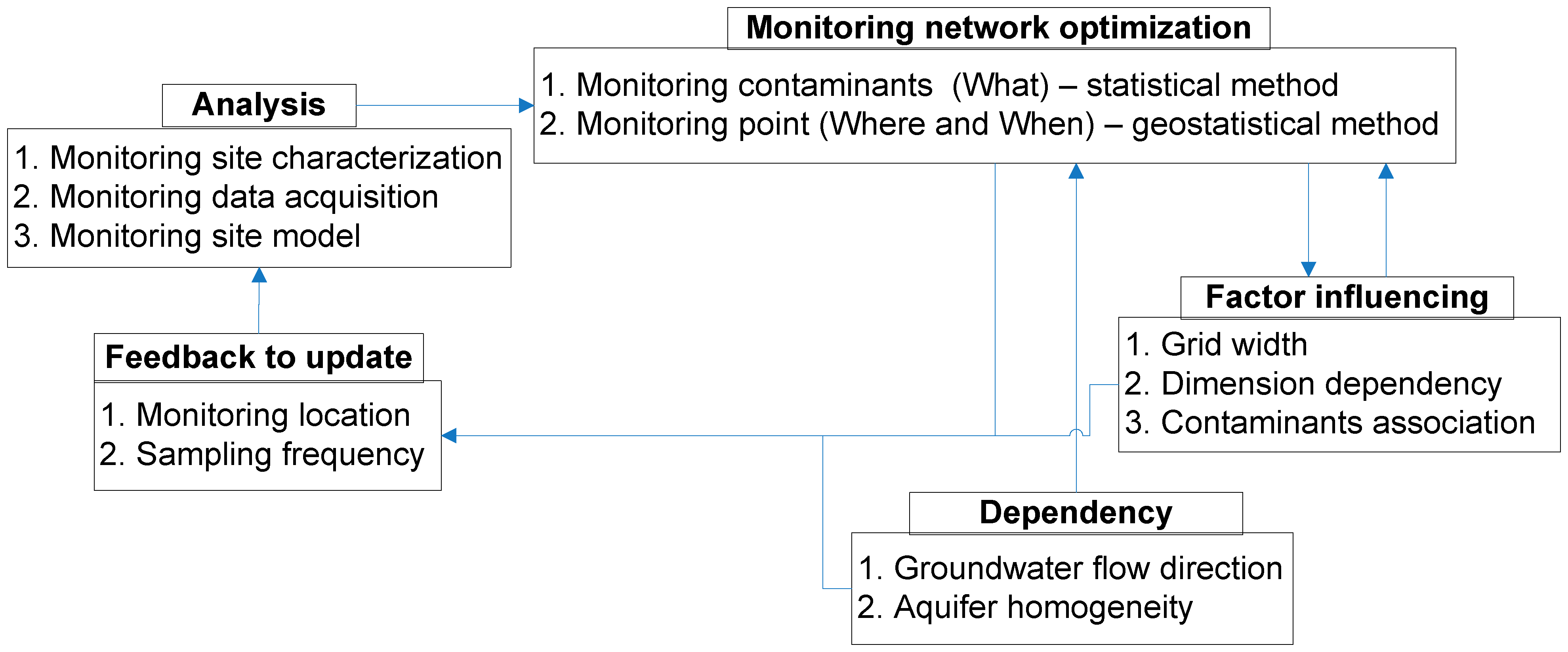
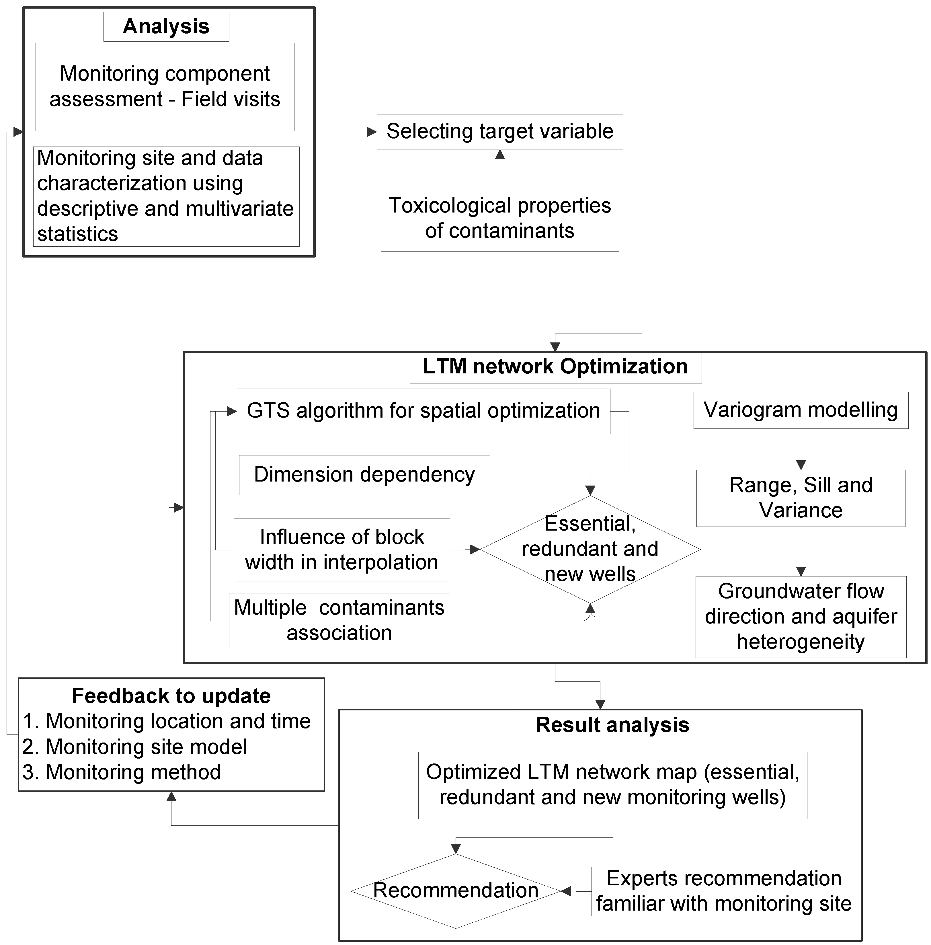
Design and improvement of monitoring strategies requires the description of its components. The components of groundwater monitoring strategy, analyzed for monitoring scenario in the study area, is represented in the logic diagram (Figure 2).

Among the groundwater physicochemical properties and contaminants concentration data, representative contaminants were first identified and then prioritized for inclusion in the monitoring strategy. Their associated uncertainties along with spatial and temporal variance were incorporated.

3.1. Selecting the Representative Variable

Identification of monitoring components in the research area was done through Principal Component Analysis (PCA). PCA of the normalized variables was performed to extract significant PCs. The variables were standardized through z-scale transformation to avoid misclassification due to difference in data dimensionality [26,27]. PCA provides information about the principle variables responsible for spatial variation in groundwater quality [28].

Figure 2. Logic diagram showing components of groundwater monitoring strategies as a circular continuous process.

Figure 2. Logic diagram showing components of groundwater monitoring strategies as a circular continuous process.

Measures of descriptive statistics in conjunction with statistical modelling of all available water quality and contaminant concentration data were used to identify the representative contaminants. World Health Organization (WHO) standards for drinking water and maximum contamination limit (MCL) of pollutants and contaminant concentration as well as associated human health risk were considered in the course of identification of the representative contaminants [29,30].

3.2. LTM Network Optimization

Necessary information about contaminants, including their properties, hydro-geochemical properties of aquifers, and other related information, are the pre-requisites for optimization of LTM network. Representative contaminants in the study area were MCB, SO₄^{2 −}and α-HCH, which was identified based on PCA that was used for monitoring network optimization. MCB and SO₄²⁻ represent organic and inorganic contamination respectively in the research area [31,32]. α-HCH, which is an organochloride and one of the isomers of hexachlorocyclohexane (HCH), represents pesticides [33,34].

3.2.1. Spatial Optimization Methods

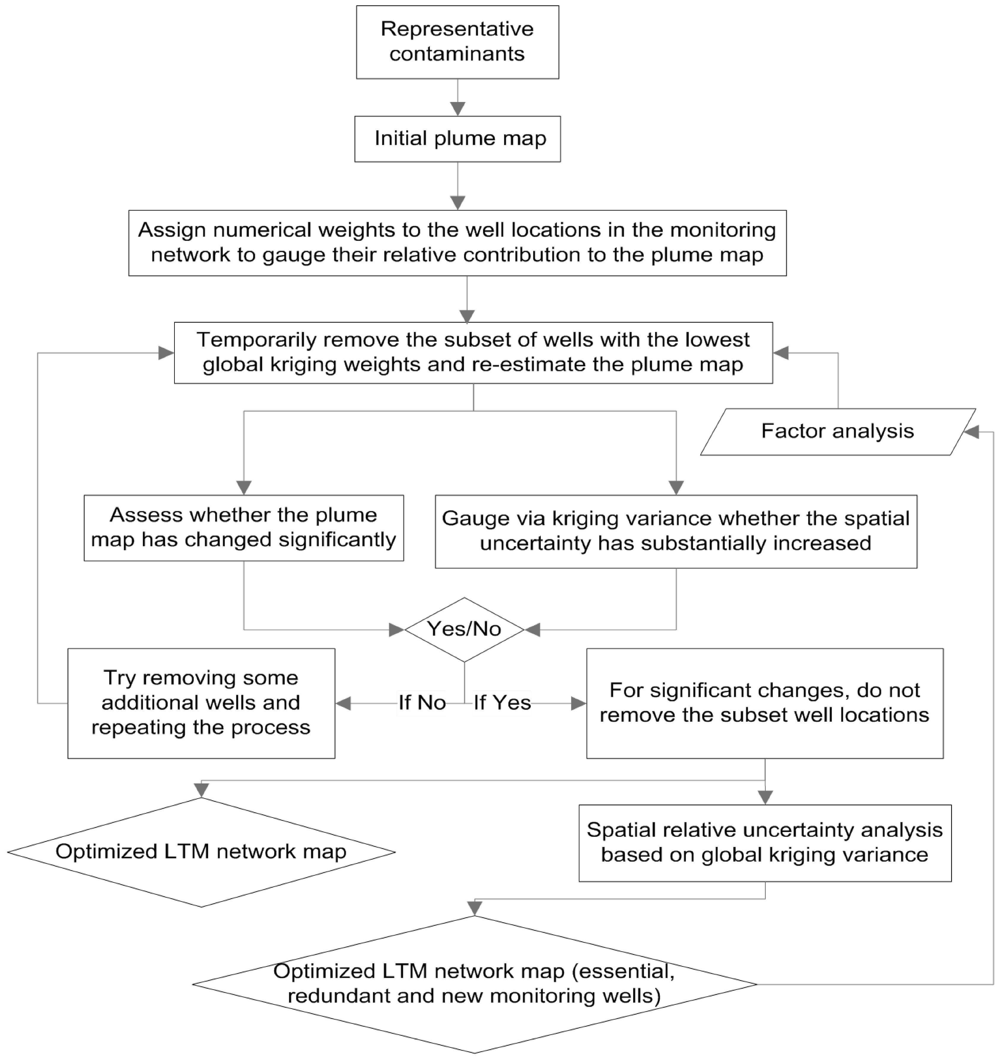
Redundant wells were predicted using Geostatistical Temporal-Spatial algorithm (GTS) on a concrete basis that the remaining wells represent the same amount of statistical information about the underlying plume [35,36]. GTS concept considers a well or its group redundant if it plays insignificant contribution to the interpolated map of contaminant plumes. The investigation steps involved in locating essential and redundant wells are shown in Figure 3.

An interpolated contaminant concentration plume was generated with input data of MCB, α-HCH and SO₄²⁻ at specified locations of the well. The maximum concentration limit (MCL) for each contaminant i.e., 100 μg/L, 0.2 μg/L and 0.25 g/L respectively for MCB, α-HCH and SO₄²⁻ [30] was given as input indicator limit to the statistical algorithm. The contaminant concentration was converted into an indicator value as

i_C(t) = 1 if z(t) > C and 0 if z(t) ≤ C

(1)

where, i_C(t) is the indictor value, z(t) is the concentration at time t, and C is the maximum contamination limit (MCL).

Figure 3. Research steps to locate essential and redundant wells and to propose new wells in the existing monitoring network (Modified from Cameron and Philip M. Hunter (2010) [36]).

Figure 3. Research steps to locate essential and redundant wells and to propose new wells in the existing monitoring network (Modified from Cameron and Philip M. Hunter (2010) [36]).

Once again, to take into account the correlation based on distance and direction between pairs of sampling locations for each contaminant, the empirical variogram was modelled. The empirical spatial variogram, γ, as a function of lag distance can be expressed as:

$$\gamma (\Delta h)=\frac{1}{2N(\Delta h)}{{\displaystyle \sum _{i.j||x_j-x_i|-\Delta h||\le \epsilon }\left[i_C(x_j)-i_C(x_i)\right]}}^2$$

(2)

where Δh is the targeted lag distance and may depend on direction; x_i and x_j are the ith and jth monitoring well locations; and N(Δh) is the number of indicator pairs contributing to the summation for lag Δh.

Numerical weight was given to the wells based on global kriging and a plume map was generated for the monitoring network. For this process, two intermediate computations were carried out:

(i) the local kriging weights of sampled locations which were processed to generate a “global” interpolation weight for each well [37]; and (ii) the local kriging estimation variance which indicate the relative uncertainty of the local block estimates in comparison to the estimates at other blocks [36].

Spatial-temporal algorithm incorporates series of procedural steps to estimate global interpolation weight and the local kriging estimation variance. At first, the study area is divided into sets of non-overlapping blocks. The set of closest sampled locations is then located at each block with the help of simple search algorithm. Then, local kriging weights (λ^B) is computed for each well based on the spatial configuration of known indicator value within and surrounding the block as well as spatial correlation between average block location and each known indicator by using modelled spatial covariance function.

A block indicator estimate is then generated with the combination of local weights and indicator values. A block indicator estimate consist of weighted average of the n(x_B) indicators located within the search radius of the block (x_B), which is estimated as [36]:

$$i_C(x_B)={\displaystyle \sum _{i=1}^{n(x_B)}{\lambda }_i^B{i}_C(x_i)}$$

(3)

for x_i ϵ search radius of block x_B.

Global interpolation weights (λ^G) is generated by averaging the local kriging weights to the given well that can be used to estimate the well’s overall contribution to the interpolated map [36], and are given by:

$${\lambda }^G(x_i)=\frac{1}{N_B}{\displaystyle \sum _{B=1}^{N_B}{\lambda }_i^B(x_i)}$$

(4)

where N_B is the total estimated number of blocks and x_i is the location of the ith sampled well.

The global kriging weights provide relative rankings of well locations in terms of independent spatial information which gives a logical interpretation that the wells with the lowest global kriging weights are predominantly spatially redundant wells. If the temporary removal of the subsets of these wells does not significantly affect the nature of plume map, these wells were permanently removed. This process is repeated until the removal of a subset of wells change the plume map. Performing this process subsequently creates a situation where the removal of subsets significantly changes the plume. At this point in time, the subset is not removed from the network. In order to fix the limitation for such changes in plume map, a two-sided (upper and lower) confidence interval of 95% is assigned while limiting median plume concentration.

Again, the relative spatial uncertainty for the installation of new monitoring wells in the existing LTM network based on the local kriging variance is given by the global kriging variance (kv^G), defined as:

$${\text{kv}}^{\text{G}}=\frac{1}{N_B}{\displaystyle \sum _{B=1}^{N_B}k{v}^B(x_B)}$$

(5)

where x_B denotes the location of the Bth block and kv^B (x_B) is the local kriging variance of the Bth block [36].

The groundwater LTM network has been spatially optimized for MCB, α-HCH and SO₄²⁻ in 2-D and 2.5-D of the groundwater aquifer. The inherent assumption in 2-D analysis is the existence of all well locations in flat 2-D which is most applicable with a single, fairly uniform and well-connected aquifer. In contrast, the 2.5-D analysis assumes multiple hydrogeological layers in the aquifers without hydraulic interconnection in which LTM is optimized for separate hydrogeological layers. The Quadratic Logistic Regression (QLR) mapping algorithm then uses the data (segregated into subsets representing one chemical of concern for each vertical zone and time slice triplet) from a given subset to map the layer and time frame represented by that given triplet.

3.2.2. Temporal Optimization Method

To optimize groundwater monitoring network temporally, Sen’s method [38] was applied which is based on iterative thinning. The algorithm consists of (i) estimating a trend using the entire time series; (ii) thinning the time series by a randomly selected fraction of the measurements; and then (iii) re-estimating the trend to determine if the slope estimate is still close to the original slope. The random removal is only retained if the measured slope is within the limits of the confidence interval on the slope using the full dataset [36]. To eliminate the effect of statistical assumptions inherent in standard linear regression methods, trend estimation is carried out using Sen’s method [38,39]. Sen’s procedure is non-parametric, readily adapted to non-detect measurements and irregular sampling frequencies [40]. Furthermore, this method precludes the calculation of slope for missing points and can predict the median slope even if the number of undetected measurements is less than (n − 1)/2.

Sen’s estimate (Q) is simply the median value of the resulting list of slopes and is given by:

$$\text{Q}=\frac{x_j-x_i}{j-i}$$

(6)

Q is the slope between data points; x_i and x_j are concentrations measured at times i and j; Time j is after time i (j > i).

Q = median slope = Q_{[(N + 1)/2]} if N is odd = (Q_[N/2] + Q_{[(N + 2)/2]})/2 if N is even

(7)

where N is the number of calculated slopes

A two side (M₁, upper and M₂, lower) confidence interval for the median slope is estimated using Z_statistic and Mann-Kendall statistic (VAR(S)). If there is a two-sided confidence interval of 95%, the Z_(1−0.05/2) = Z_0.975 = 1.96. Mann-Kendall statistic (VAR(S)) [41,42] is given by:

$$VAR\left(S\right)=\frac{1}{18}\left[n\left(n-1\right)\left(2n+5\right)-{\displaystyle \sum }_{p-1}^q{t}_p(t_p-1)(2t_p+5)\right]$$

(8)

where n is number of sampling data points, t_p is the number of ties for the pth value and q is the number of tied values. Equation (8) may be used for values between 10 and 40. The range of ranks for the specified confidence interval (C_i) [38] is given as shown below:

$$C_i=Z_{1-i/2}\times \sqrt{VAR(S)}$$

(9)

Taking the value of Equation (9), the ranks of the lower (M₁) and upper (M₂ + 1) confidence limits can be calculated using the following relation:

$$M_1=\frac{N-C_i}{2} \text{And }{M}_2=\frac{N+C_i}{2}$$

(10)

The values of lower (M₁) and upper (M₂ + 1) confidence limits were used to define lower and upper boundaries along the median slope. The temporal optimization of the existing groundwater monitoring network was carried out using α-HCH, MCB and SO₄²⁻ concentration data set from 2003–2009 for each contaminant separately and together.

3.3. Factors Influencing Monitoring Optimization Results

3.3.1. Block Width and Dimension Dependency

In the monitoring network optimization using geostatistical methods, a plume map of well location is created with the help of global kriging weight [8] computed by interpolation method which depends upon width and number of blocks. Hence, in the optimization process, a block width from 1000 m to 1 m was demarcated in order to discover ambiguities in the method.

The 2-D treatment ignores the sampling depth of monitoring well while in the 2.5-D case, the aquifer is assumed to have the number of hydrogeological layers and thus the sampling depth of the monitoring wells needs to be taken into account. For systematic study of the influence of dimension and block width on monitoring network optimization methods, the optimization process has considered block widths from 1000 m to 1 m in both 2 and 2.5 dimensions.

3.3.2. Contaminants Association

Based on PCA of hydro-geochemical data, contaminant concentration of three representative variables, α-HCH, MCB and SO₄²⁻ are used individually to monitor network optimization. The likely influence of multiple variables on optimization process is examined using data sets in groups as well as all three variables together. In this case, co-kriging was used to compute co-kriging numerical weights from contaminant concentrations for each monitoring well which in turn were used to create a plume map of the monitoring network which is used for geostatistical optimization of monitoring network as explained in Section 3.2.1.

3.4. Groundwater Flow Direction and Aquifer Homogeneity

In addition to spatio-temporal optimization of ground water monitoring network, direction of ground-water flow and homogeneity of the aquifer was determined. Groundwater flow direction is known to play a prominent role in monitoring network optimization. The directional dependency was studied using directional variograms. Estimation of experimental variogram was carried out using Golden Surfer software [43].

Since variograms based on contaminant concentration data set were anisotropic in nature, valid variogram model incorporating directional dependence were constructed using standard models to model the data set. The best fitting model, considering range, sill, nugget effect and shape of the model, was selected. A variogram was built from a concentration data set of α-HCH, MCB and SO₄²⁻ for the years 2003–2009, according to seasons (summer: May–October; winter: November–April) and to hydrologic seasons (March–May: High groundwater level, September–November: Low groundwater level). The range and sill were estimated for various directional variogram models.

A homogeneity index (RV index) which numerically estimates homogeneity of the aquifer was defined based on range, sill and variance of the variogram [44] based on the variogram model as given by:

$$\text{Homogeneity index}=\frac{\text{range}}{\frac{sill+variance}{2}}$$

(11)

3.5. Integrating Approaches and Improving Groundwater Monitoring Strategy

New sets of methods were analyzed with new approaches based on integrated statistical and geostatistical methods, integrated in the light of various optimization objectives. However, basic framework and components of groundwater monitoring strategies were duly taken into consideration while subjecting these methods to integration. The new integrated methods, although based on different approaches, could be used as an impeccable tool for groundwater monitoring network optimization and feedback for updating groundwater monitoring strategies. While integrating these methods, the advantages and disadvantages of the methods being used have also been analysed.

4. Results

4.1. Representative Variable in the Research Area

For the purpose of dimension reduction and analysis of major components loading the system, PCA was applied to a matrix of hydro-geochemical data. The first four principal components in this dataset with eigenvalues greater than one explain 66% of the cumulative variance. The significance of the parameters in four components was further depicted by the component matrix extracted with PCA and varimax with the Kaiser Normalization rotation method. At 75% significance level, SO₄²⁻, Fe, pH and Eh play a major role in the system whereas α-HCH and MCB are minor components. In the first component, SO₄²⁻ and Fe have positive loading. In the second component, Eh has positive loading. However, pH is has negative loading because the acidic groundwater environment in the study area arises from a high SO₄²⁻ concentration. SO₄²⁻ and Fe have positive loading in the first component whereby Eh has positive loading in the second component. The negative loading of pH could be linked to the acidic groundwater environment in the study area from high SO₄²⁻ concentration.

4.2. Optimization of LTM Network

4.2.1. Spatial Optimization of LTM Network

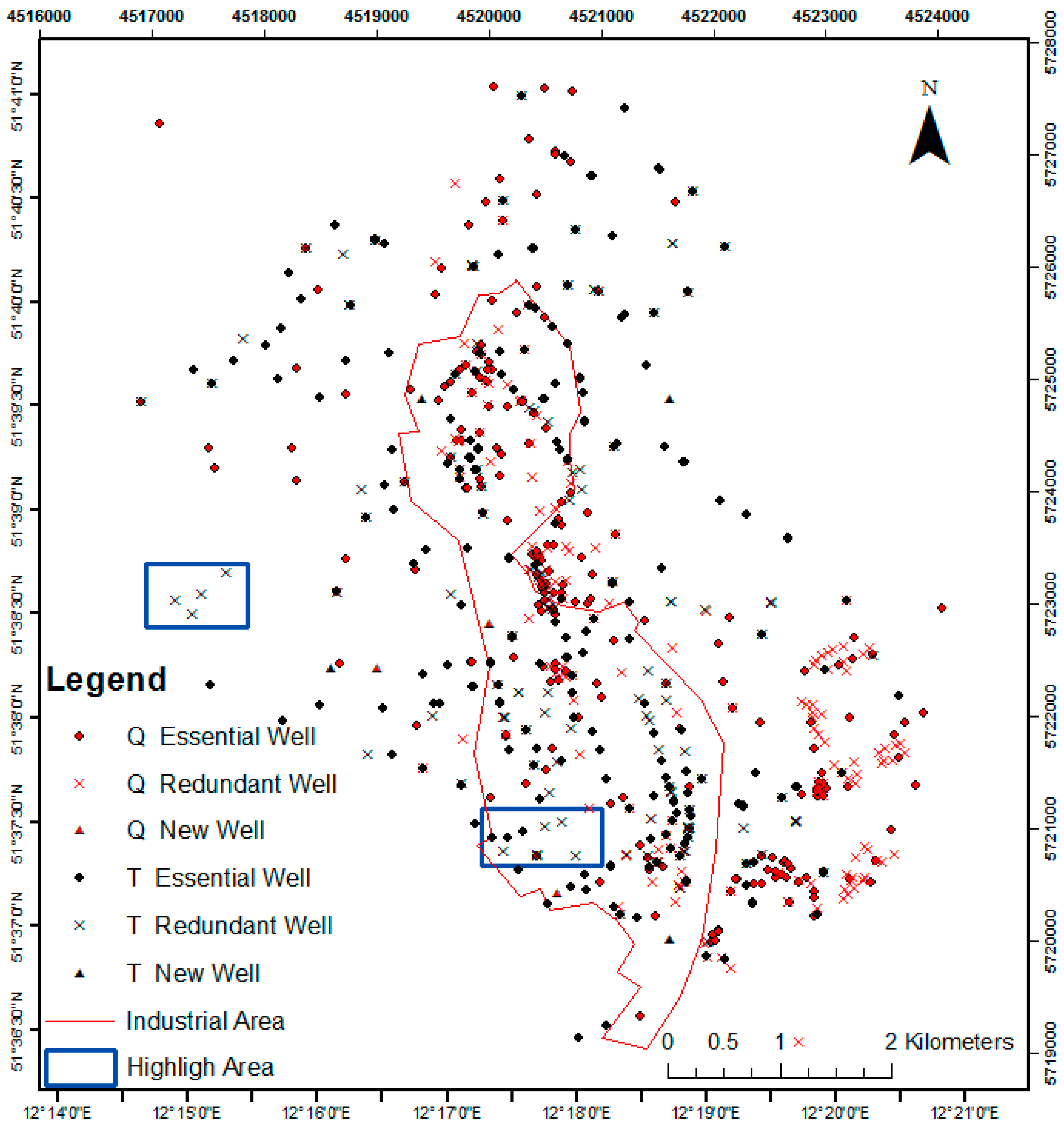
Both types of aquifers were considered separately during the spatial optimization of LTM network in accordance with the methods described in Section 3.2. The optimized monitoring network suggests 292 wells out of 462 wells in the Quaternary aquifer and 256 wells out of 357 wells in the Tertiary aquifer for monitoring needs at the suggested temporal interval.

The spatial uncertainties analysis, resulting from the global kriging variance (using Equation (5)) made recommendations for 22 and 41 new monitoring wells, respectively, in the Tertiary and Quaternary aquifers. The spatial distribution of redundant, essential, and proposed new wells in the Quaternary and Tertiary aquifer is depicted in Figure 4. Similar kriging weights in the original and optimized LTM network datasets points out that reduction in observation points does not compromise the quality or resolution of the collected samples as long as the distribution is logically and conveniently designed.

Figure 4. Optimized LTM network map showing location of essential, redundant, and proposed new wells in the monitoring network.

Figure 4. Optimized LTM network map showing location of essential, redundant, and proposed new wells in the monitoring network.

4.2.2. Temporal Optimization of LTM Network

Monitoring network was temporally optimized through statistical approach using Sen’s method, with 95% confidence intervals around the slope estimates, as described in Section 3.2.2. The outputs from temporal optimization are the sampling intervals at 3 quartiles (lower, median and upper) for individual monitoring well and each monitoring parameter (Table 2). The optimization results reveal that the optimization differs remarkably while considering pair and multiple contaminants.

Table 2. Temporal optimization of monitoring network in Quaternary and Tertiary aquifer for monochlorobenzene (MCB), α-HCH and SO₄²⁻.

V. Zone	COC	Present Sampling Interval (Days)			Recommended Sampling Interval (Days)
		Lower Quartile	Median Quartile	Upper Quartile	Lower Quartile	Median Quartile	Upper Quartile
Q	MCB	92	210	254	205	328	503
Q	α-HCH	138	181	224	298	327	418
Q	SO42−	179	217	268	325	506	704
T	MCB	143	221	280	282	443	810
T	α-HCH	224	224	224	342	398	553
T	SO42−	188	217	278	435	589	836
Q	all	138	210	254	298	328	503
T	all	188	221	278	342	443	810
Both	all	161	217	261	311	420	628

Note: Q: Quaternary aquifer; T: Tertiary aquifer; COC: Chemical of Concern.

Table 2. Temporal optimization of monitoring network in Quaternary and Tertiary aquifer for monochlorobenzene (MCB), α-HCH and SO₄²⁻.

V. Zone	COC	Present Sampling Interval (Days)			Recommended Sampling Interval (Days)
		Lower Quartile	Median Quartile	Upper Quartile	Lower Quartile	Median Quartile	Upper Quartile
Q	MCB	92	210	254	205	328	503
Q	α-HCH	138	181	224	298	327	418
Q	SO42−	179	217	268	325	506	704
T	MCB	143	221	280	282	443	810
T	α-HCH	224	224	224	342	398	553
T	SO42−	188	217	278	435	589	836
Q	all	138	210	254	298	328	503
T	all	188	221	278	342	443	810
Both	all	161	217	261	311	420	628

Note: Q: Quaternary aquifer; T: Tertiary aquifer; COC: Chemical of Concern.

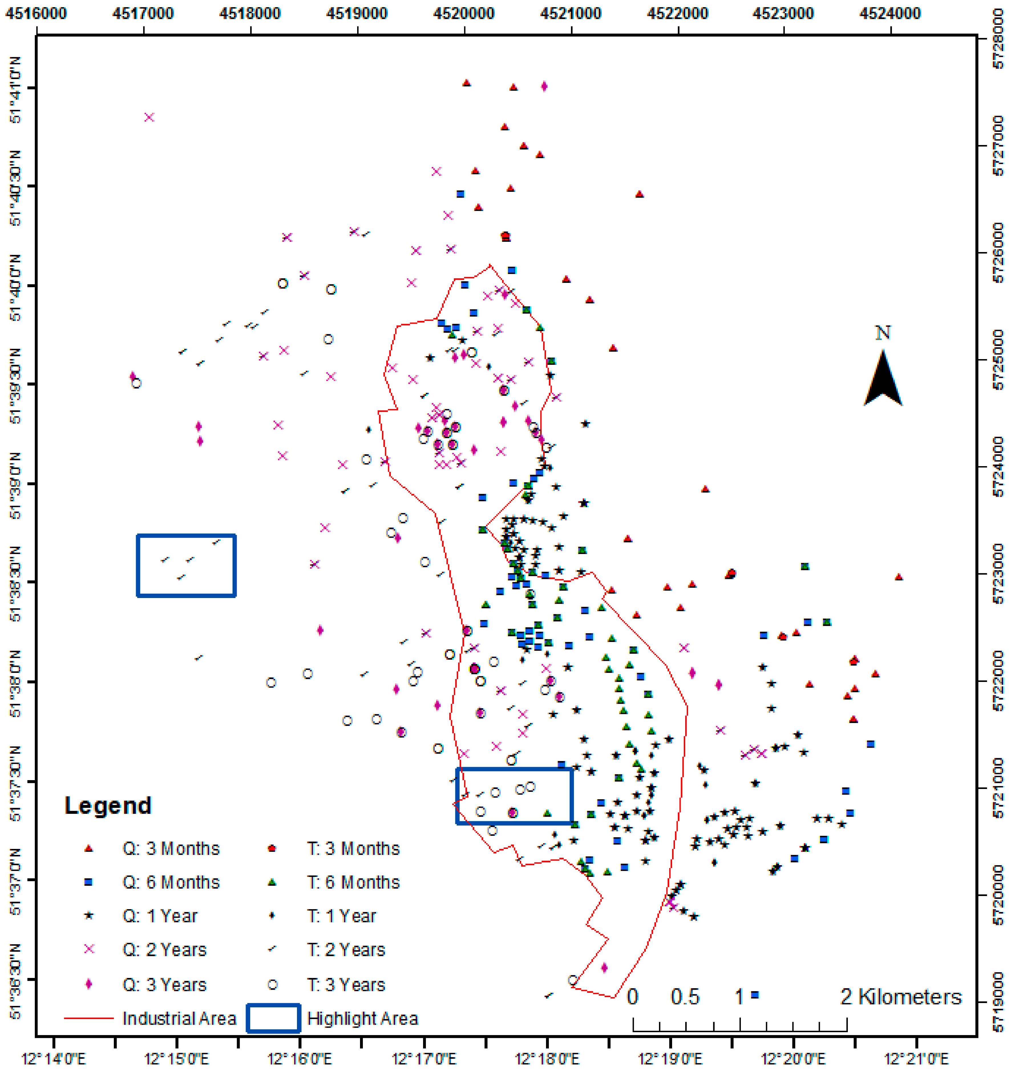
In order to clearly visualize and precisely describe the temporal optimization results of three contaminants in combination, the recommended median quartile sampling frequency for the monitoring wells was divided into five classes: three months, six months, one year, two years and three years. Recommendations for specific number of monitoring wells with respect to each of the categorized temporal sampling interval are specified in Table 3.

Table 3. Number of monitoring wells for each sampling interval.

Sampling Interval	3 Months	6 Months	1 Year	2 Years	3 Years	Total
Quaternary	34	86	173	76	93	462
Tertiary	16	69	114	84	74	357
Total No. of wells	50	155	287	160	167	819

Table 3. Number of monitoring wells for each sampling interval.

Sampling Interval	3 Months	6 Months	1 Year	2 Years	3 Years	Total
Quaternary	34	86	173	76	93	462
Tertiary	16	69	114	84	74	357
Total No. of wells	50	155	287	160	167	819

Figure 5 shows the distribution of monitoring wells and their recommended sampling intervals. The highest number of sampling wells is recommended at the yearly sampling interval.

In the study area, the overall temporally optimized sampling interval was recommended as 238 days, 317 days and 401 days in terms of lower, median and upper quartiles respectively.

4.3. Factor Influencing Monitoring Optimization Results

4.3.1. Dimension and Block Width Dependency

With an objective of incorporating dependency of dimension and block width on optimization process, the optimization was carried out for different interpolation block widths (from 1000 m to 1 m) for both aquifers in both 2 and 2.5 D dimensions as described in Section 3.3.1.

Figure 5. Statistically temporally optimized LTM network map showing recommended temporal frequency of the monitoring wells in the monitoring network.

Figure 5. Statistically temporally optimized LTM network map showing recommended temporal frequency of the monitoring wells in the monitoring network.

Optimization in 2-D Aquifer

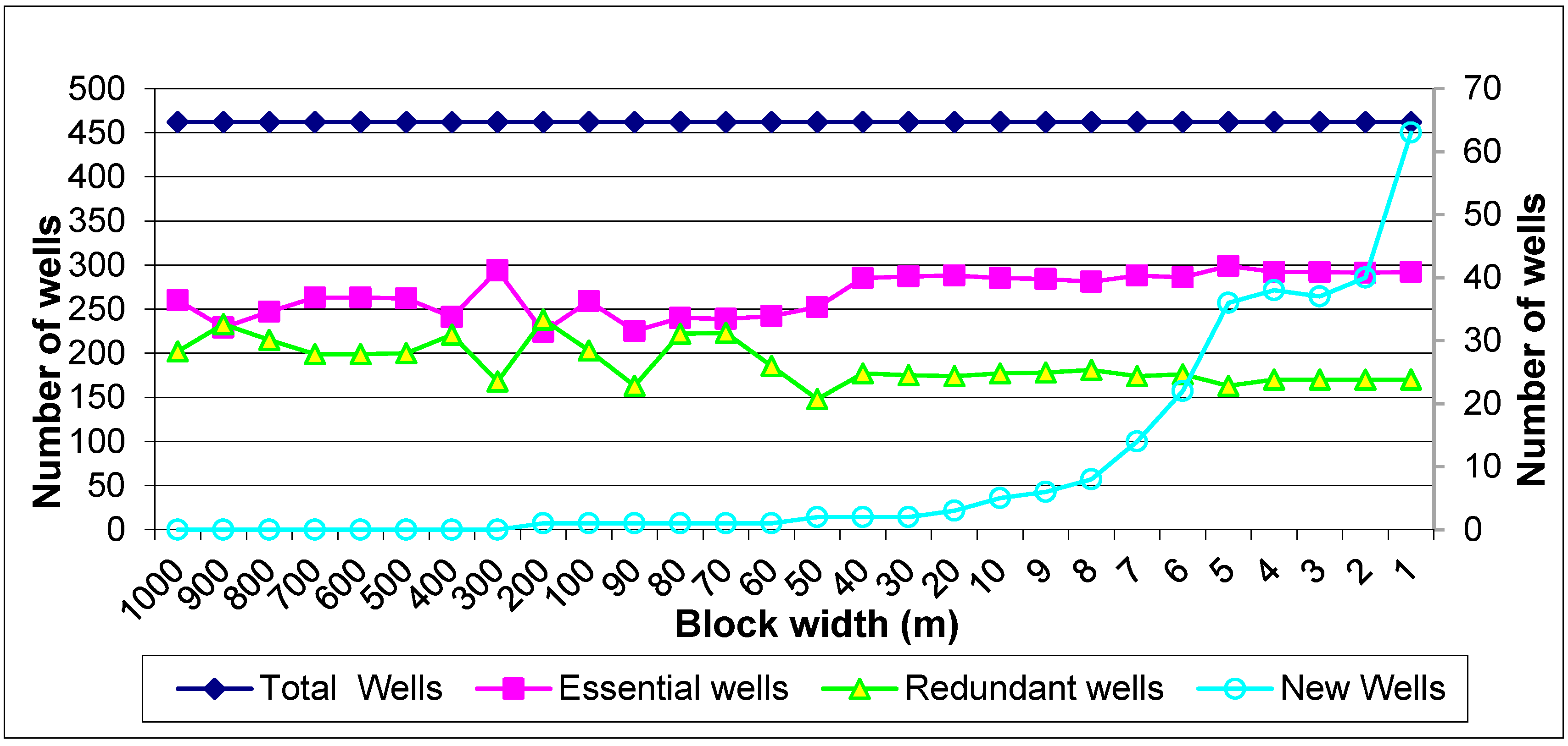
Considering the aquifer as a 2-D plain, groundwater monitoring network was spatially optimized for MCB, α-HCH and SO₄². The result unveiled a significant change in number of suggested/essential wells as well as existing redundant wells with changing block width for interpolation (from 1000 m to 1 m). The increase in the relative spatial uncertainties based on local kriging variance with decreasing block width eventually recommends installation of new monitoring wells.

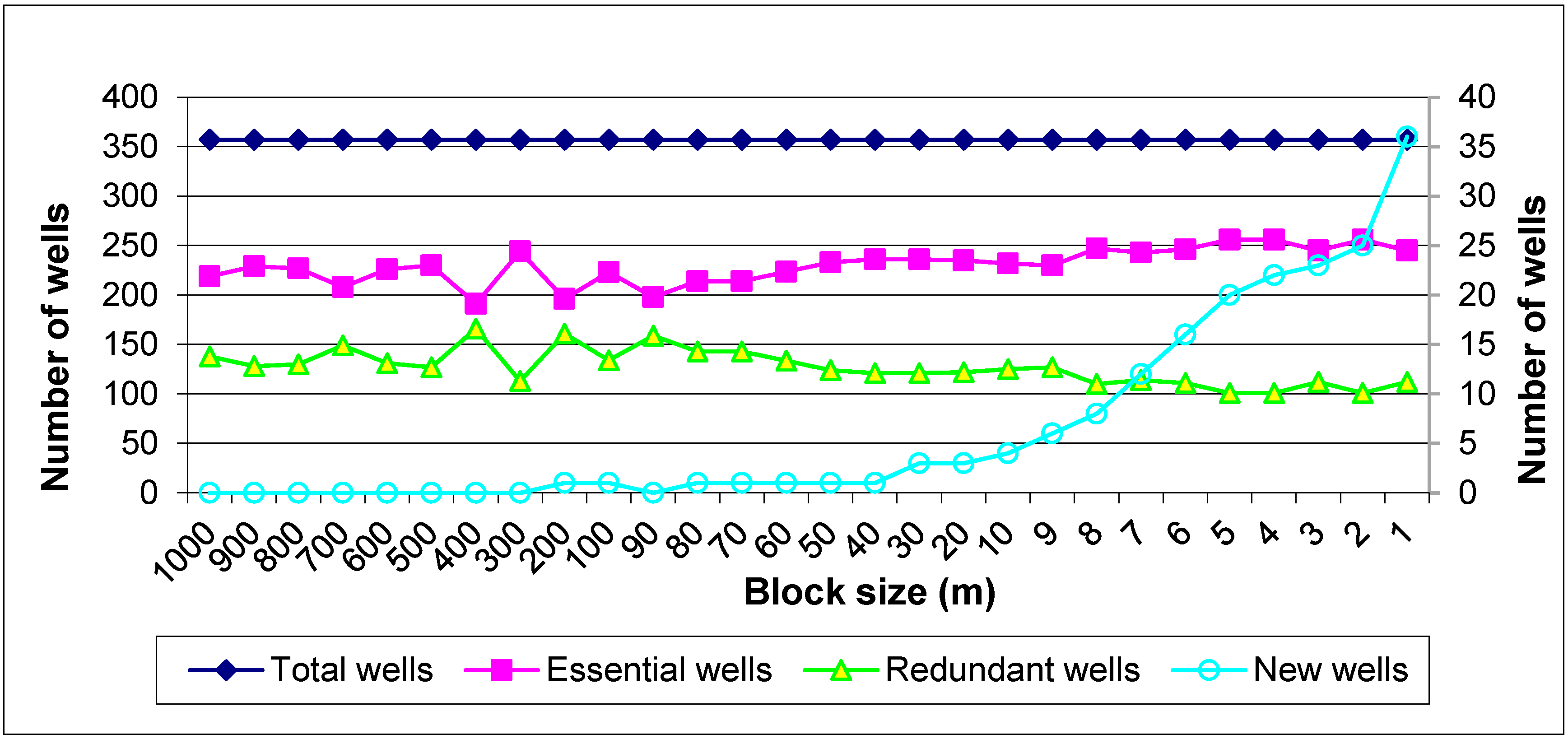
The overall analysis of optimization in 2-D plain unveils that the relative spatial uncertainty increases with decreasing block width from 200 m to 1 m in both aquifers (Figure 6 and Figure 7), thus suggesting the need of installation of 63 and 36 new wells, respectively, in Quaternary and Tertiary aquifers at 1 m block width.

Figure 6. Block width dependency in the LTM network optimization in the Quaternary aquifer for MCB, α-HCH and SO₄²⁻ in a 2-D plain. Essential, redundant and total number of wells is on left Y-axis and number of new wells is on right Y-axis.

Figure 6. Block width dependency in the LTM network optimization in the Quaternary aquifer for MCB, α-HCH and SO₄²⁻ in a 2-D plain. Essential, redundant and total number of wells is on left Y-axis and number of new wells is on right Y-axis.

Figure 7. Block width dependency in the LTM network optimization in the Tertiary aquifer for MCB, α-HCH and SO₄²⁻ in a 2-D plain. Essential, redundant and total number of wells are on left Y-axis and the number of new wells is on right Y-axis.

Figure 7. Block width dependency in the LTM network optimization in the Tertiary aquifer for MCB, α-HCH and SO₄²⁻ in a 2-D plain. Essential, redundant and total number of wells are on left Y-axis and the number of new wells is on right Y-axis.

Optimization in a 2.5-D Aquifer

Spatial optimization for MCB, α-HCH and SO₄²⁻ in groundwater LTM network has been conducted in combination in 2.5-D aquifer. The LTM network is optimized separately for each hydro-stratigraphic layer in the aquifer using data from that layer only.

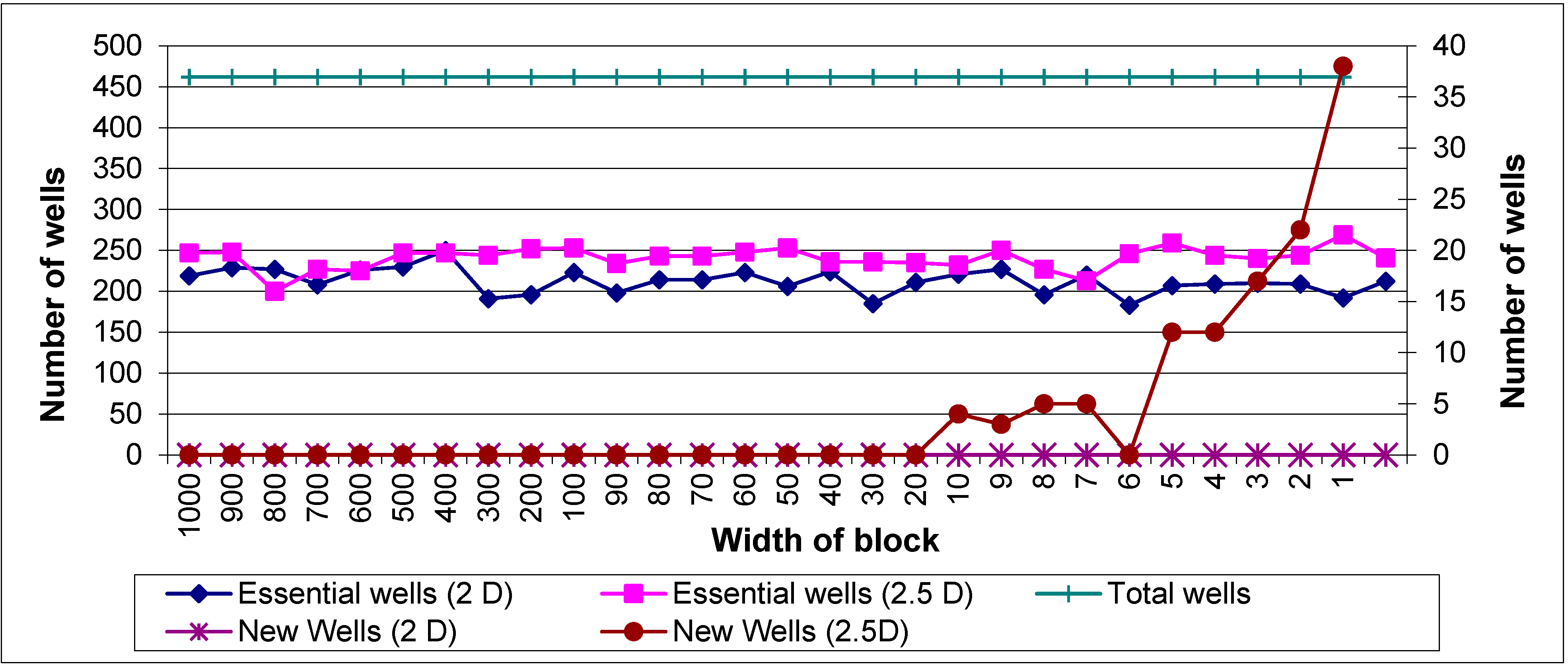
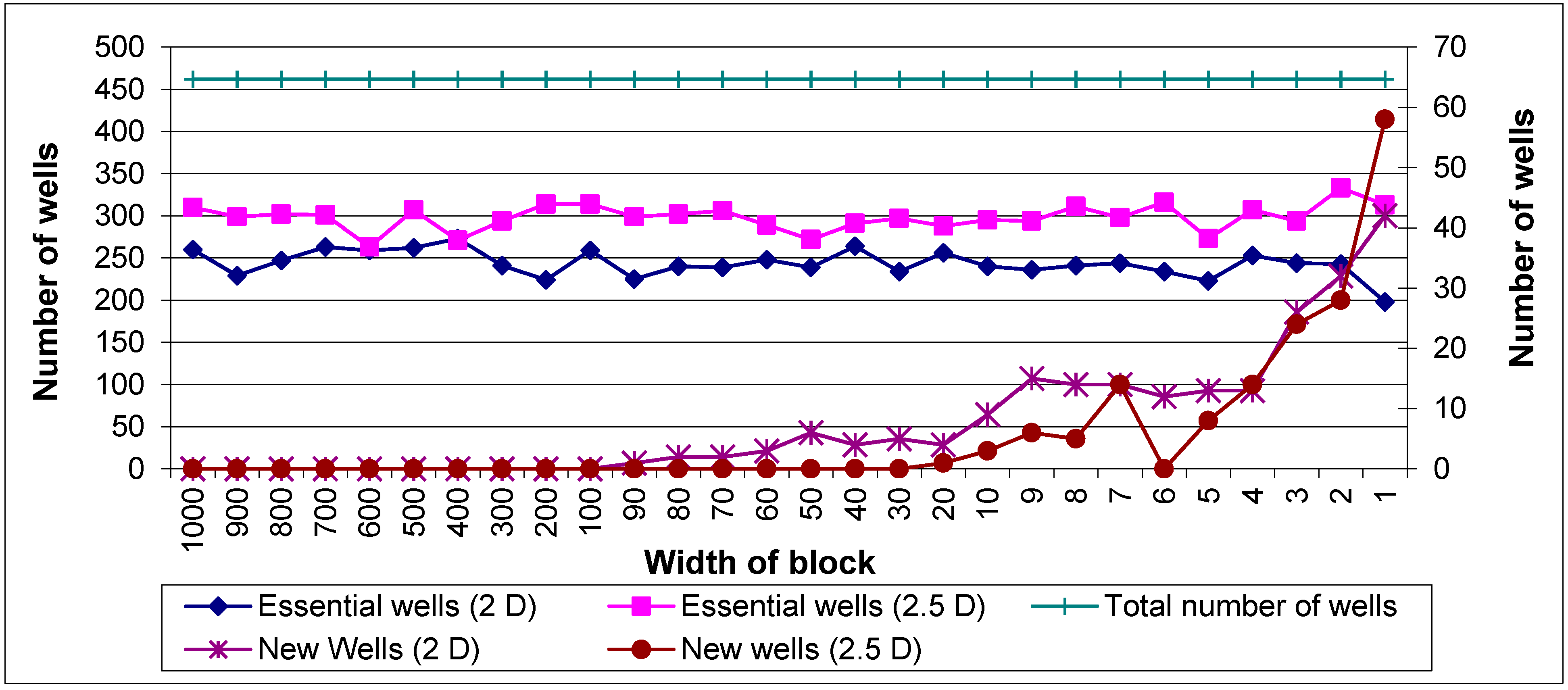
In the case when all three contaminants are considered together, the change in block width for interpolation (1000 m to 1 m) does not significantly change the number of suggested wells (Figure 8 and Figure 9). The increment of spatial relative uncertainty significantly with decreasing block width from 20 m to 1 m suggests the installation of 58 and 38 new monitoring wells in Quaternary and Tertiary aquifers, respectively.

Figure 8. Block width dependency in the LTM network optimization in the Quaternary aquifer for MCB, α-HCH and SO₄²⁻ considering 2-D and 2.5-D aquifers. Essential, redundant and total number of wells are on left Y-axis and number of new well is on right Y-axis.

Figure 8. Block width dependency in the LTM network optimization in the Quaternary aquifer for MCB, α-HCH and SO₄²⁻ considering 2-D and 2.5-D aquifers. Essential, redundant and total number of wells are on left Y-axis and number of new well is on right Y-axis.

Figure 9. Block width dependency in the LTM network optimization in the Tertiary aquifer for MCB, α-HCH and SO₄²⁻ in 2-D and 2.5-D aquifers. Essential, redundant and total number of wells are on the left Y-axis and the number of new wells is on the right Y-axis.

Figure 9. Block width dependency in the LTM network optimization in the Tertiary aquifer for MCB, α-HCH and SO₄²⁻ in 2-D and 2.5-D aquifers. Essential, redundant and total number of wells are on the left Y-axis and the number of new wells is on the right Y-axis.

4.3.2. Contaminants Association

To account for the association between the contaminants, the LTM network was spatially optimized taking 7 m interpolation block width for the contaminants MCB, α-HCH and SO₄²⁻ in pairs as well as all grouped together, considering the groundwater aquifer separately as 2-D plain and as 2.5-D aquifer. Dependency of contaminants association on network optimization is supported by result that the spatial optimizations of the LTM network for MCB and α-HCH individually show less redundancy and low recommendations for new monitoring wells while that only for SO₄²⁻ recommends higher number of redundant wells (70%). Such effect of incorporating greater number of contaminants is presented in Table 4 and Table 5. For example, in the Quaternary aquifer considered as a 2-D plain, for α-HCH and SO4²⁻, 73 wells are recommended, for MCB and SO₄², 293 wells are recommended and for MCB and α-HCH, 335 wells are recommended. However, 244 wells are recommended when considering all three contaminants MCB, SO₄²⁻ and α-HCH together (Table 4). Similarly, in the tertiary aquifer considered as a 2.5-D plain, 72, 267, 247 and 213 wells are recommended, respectively, for combination of α-HCH and SO₄²⁻; MCB and SO₄²⁻; MCB and α-HCH; and MCB, SO₄²⁻ and α-HCH together (Table 5).

Table 4. Number of essential, redundant and new well location recommendation from 2-D groundwater monitoring network optimization for α-HCH and SO₄²; MCB and SO₄²⁻; MCB and α-HCH; and MCB, SO₄²⁻ and α-HCH in Quaternary (462 wells) and Tertiary (357 wells) aquifers.

Quaternary Aquifer/Contaminants	α-HCH and SO42−	MCB and SO42−	MCB and α-HCH	MCB, SO42− and α-HCH
Essential well	73	293	335	244
Redundant well	351	169	127	218
New well location	14	7	14	14
Tertiary Aquifer
Essential wells	52	233	247	220
Redundant well	302	124	110	137
New well location	0	0	0	0

Table 4. Number of essential, redundant and new well location recommendation from 2-D groundwater monitoring network optimization for α-HCH and SO₄²; MCB and SO₄²⁻; MCB and α-HCH; and MCB, SO₄²⁻ and α-HCH in Quaternary (462 wells) and Tertiary (357 wells) aquifers.

Quaternary Aquifer/Contaminants	α-HCH and SO42−	MCB and SO42−	MCB and α-HCH	MCB, SO42− and α-HCH
Essential well	73	293	335	244
Redundant well	351	169	127	218
New well location	14	7	14	14
Tertiary Aquifer
Essential wells	52	233	247	220
Redundant well	302	124	110	137
New well location	0	0	0	0

Table 5. Number of essential, redundant and new well location recommendation from 2.5-D groundwater monitoring network optimization for α-HCH and SO₄²; MCB and SO₄²⁻ MCB and α-HCH; and MCB, SO₄²⁻ and α-HCH in Quaternary (462 wells) and Tertiary (357 wells) aquifers.

Quaternary Aquifer/Contaminants	α-HCH and SO42−	MCB and SO42−	MCB and α-HCH	MCB, SO42− and α-HCH
Essential well	107	334	341	298
Redundant well	317	127	140	164
New well location	0	2	1	14
Tertiary Aquifer
Essential well	72	267	247	213
Redundant well	282	90	148	144
New well location	0	3	8	5

Table 5. Number of essential, redundant and new well location recommendation from 2.5-D groundwater monitoring network optimization for α-HCH and SO₄²; MCB and SO₄²⁻ MCB and α-HCH; and MCB, SO₄²⁻ and α-HCH in Quaternary (462 wells) and Tertiary (357 wells) aquifers.

Quaternary Aquifer/Contaminants	α-HCH and SO42−	MCB and SO42−	MCB and α-HCH	MCB, SO42− and α-HCH
Essential well	107	334	341	298
Redundant well	317	127	140	164
New well location	0	2	1	14
Tertiary Aquifer
Essential well	72	267	247	213
Redundant well	282	90	148	144
New well location	0	3	8	5

In the optimization of LTM network for combination of three contaminants, the local kriging weight of each contaminant is averaged, which clearly depicts the dependence of relative spatial uncertainty with the spatial distribution of each contaminants. It has been observed that optimization for each type of aquifer considering individual contaminants and in groups gives recommendations for different numbers and locations of new wells (Table 4 and Table 5).

4.4. Groundwater Contaminants Flow Direction and Aquifer Homogeneity

Geostatistical and flow direction modeling methods have been used to predict the groundwater flow direction and integrate its effect into LTM network optimization. The spatial characterization of the groundwater contamination scenario (degree of spatial co-relation between contaminant concentration values) was observed using an experimental variogram exhibiting the contaminant concentration data of MCB, α-HCH and SO₄²⁻.

The geometric anisotrophy as depicted by the experimental variogram was observed for each 30° of lag direction with reference to North direction. Again, the heterogeneity in the nature of geological formation was quantified by using a homogeneity index called RV Index (Equation (11)), which takes its base from spatial variability of contaminant concentration distribution.

4.4.1. Contaminant Wise Variogram Modelling

Based on the results from experimental variogram, geometrical anisotropy was observed in the data set of α-HCH, as range and sill differed in different directions.

The experimental variogram (incorporating each 30° of lag direction) revealed the highest range in Northern direction (0°) which is also coherent with the results from RV index that was highest in the Northern direction for Quaternary aquifer (Table 6). Meanwhile, the variogram showed highest range and RV index at 30° from the Northern direction for the Tertiary aquifer (Table 6). These results specify that the overall conspicuous concentration of α-HCH flowed towards the North in both aquifers. In case of Tertiary aquifer, there was slight deviation in the flow towards east direction.

Table 6. Directional variogram modelling α-HCH concentration in the long term monitoring network (LTM) network in Quaternary and Tertiary aquifers (January 2003 to February 2009).

α-HCH for Quaternary Aquifer (2003–2009)				α-HCH for Tertiary Aquifer (2003–2009)
Model: Gaussian, Variance: 0.62				Model: Gaussian, Variance: 0.57
Direction	Range	Sill	RV Index	Direction	Range	Sill	RV Index
Omni	404	0.64	641.27	Omni	1182	0.70	1862.88
0	666	0.62	1074.19	0	960	0.79	1416.97
30	464	0.64	736.51	30	1340	0.67	2161.29
60	385	0.66	601.56	60	999	0.69	1591.91
90	321	0.66	501.56	90	710	0.70	1118.11
120	360	0.65	566.93	120	722	0.70	1137.01
150	433	0.63	692.80	150	750	0.68	1200.00
180	590	0.62	951.61	180	960	0.69	1529.76

Table 6. Directional variogram modelling α-HCH concentration in the long term monitoring network (LTM) network in Quaternary and Tertiary aquifers (January 2003 to February 2009).

α-HCH for Quaternary Aquifer (2003–2009)				α-HCH for Tertiary Aquifer (2003–2009)
Model: Gaussian, Variance: 0.62				Model: Gaussian, Variance: 0.57
Direction	Range	Sill	RV Index	Direction	Range	Sill	RV Index
Omni	404	0.64	641.27	Omni	1182	0.70	1862.88
0	666	0.62	1074.19	0	960	0.79	1416.97
30	464	0.64	736.51	30	1340	0.67	2161.29
60	385	0.66	601.56	60	999	0.69	1591.91
90	321	0.66	501.56	90	710	0.70	1118.11
120	360	0.65	566.93	120	722	0.70	1137.01
150	433	0.63	692.80	150	750	0.68	1200.00
180	590	0.62	951.61	180	960	0.69	1529.76

The relatively lower RV index in the Quaternary aquifer than in the Tertiary aquifer shows high heterogeneity in the Quaternary aquifer.

4.4.2. Season Wise Variogram Modelling for α-HCH Data

Seasonal variability was embodied into optimization by using the data set of α-HCH for hydrological summer and winter seasons to model the experimental variogram. Periodic data from May to October (2003–2009) and November to April (2003–2009) were categorized as hydrological summer and winter seasons, respectively. Analysis of the experimental variogram, using α-HCH data for the hydrological summer season, again showed the highest range in the North direction as well as highest RV index in Northern direction for both Quaternary and Tertiary aquifers (Table 7 and Table 8). These results show that preferential groundwater flow and α-HCH concentration movement occurred in the Northern direction.

Table 7. Directional variogram modelling for α-HCH concentration in the LTM network in Quaternary aquifers for summer and winter seasons (May to October in 2003–2009).

α-HCH for Quaternary Aquifer (May to October in 2003–2009)				α-HCH for Quaternary Aquifer in Winter Seasons (Nov. to April from 2003–2009)
Model: Gaussian, Variance: 0.70				Model: Gaussian, Variance: 0.68
Direction	Range	Sill	RV Index	Direction	Range	Sill	RV Index
Omni	491	0.78	661.99	Omni	669	0.73	954.01
0	491	0.70	701.43	0	398	0.74	562.54
30	387	0.75	532.54	30	534	0.71	771.12
60	340	0.77	461.52	60	543	0.68	801.48
90	354	0.78	477.28	90	397	0.72	570.20
120	364	0.79	488.59	120	411	0.73	585.47
150	333	0.76	456.16	150	422	0.74	596.89
180	390	0.65	577.78	180	513	0.73	729.21

Table 7. Directional variogram modelling for α-HCH concentration in the LTM network in Quaternary aquifers for summer and winter seasons (May to October in 2003–2009).

α-HCH for Quaternary Aquifer (May to October in 2003–2009)				α-HCH for Quaternary Aquifer in Winter Seasons (Nov. to April from 2003–2009)
Model: Gaussian, Variance: 0.70				Model: Gaussian, Variance: 0.68
Direction	Range	Sill	RV Index	Direction	Range	Sill	RV Index
Omni	491	0.78	661.99	Omni	669	0.73	954.01
0	491	0.70	701.43	0	398	0.74	562.54
30	387	0.75	532.54	30	534	0.71	771.12
60	340	0.77	461.52	60	543	0.68	801.48
90	354	0.78	477.28	90	397	0.72	570.20
120	364	0.79	488.59	120	411	0.73	585.47
150	333	0.76	456.16	150	422	0.74	596.89
180	390	0.65	577.78	180	513	0.73	729.21

Table 8. Directional variogram modelling of α-HCH concentration in the LTM network in Quaternary and Tertiary aquifers for winter seasons (November to April from 2003–2009).

α-HCH for Tertiary Aquifer (May to October in 2003–2009)				α-HCH for Tertiary Aquifer in Winter Seasons (Nov. to April from 2003–2009)
Model: Gaussian, Variance: 0.70				Model: Gaussian, Variance: 1.25
Direction	Range	Sill	RV Index	Direction	Range	Sill	RV Index
Omni	1166	0.41	2854.69	Omni	585	1.41	439.85
0	1258	0.47	2875.43	0	579	1.31	452.34
30	1062	0.46	2455.49	30	550	1.25	440.00
60	939	0.38	2392.36	60	600	1.33	465.12
90	888	0.43	2122.12	90	850	1.26	677.29
120	737	0.43	1761.26	120	1050	1.22	850.20
150	793	0.42	1934.15	150	823	1.25	658.40
180	882	0.44	2082.89	180	526	1.32	409.34

Table 8. Directional variogram modelling of α-HCH concentration in the LTM network in Quaternary and Tertiary aquifers for winter seasons (November to April from 2003–2009).

α-HCH for Tertiary Aquifer (May to October in 2003–2009)				α-HCH for Tertiary Aquifer in Winter Seasons (Nov. to April from 2003–2009)
Model: Gaussian, Variance: 0.70				Model: Gaussian, Variance: 1.25
Direction	Range	Sill	RV Index	Direction	Range	Sill	RV Index
Omni	1166	0.41	2854.69	Omni	585	1.41	439.85
0	1258	0.47	2875.43	0	579	1.31	452.34
30	1062	0.46	2455.49	30	550	1.25	440.00
60	939	0.38	2392.36	60	600	1.33	465.12
90	888	0.43	2122.12	90	850	1.26	677.29
120	737	0.43	1761.26	120	1050	1.22	850.20
150	793	0.42	1934.15	150	823	1.25	658.40
180	882	0.44	2082.89	180	526	1.32	409.34

In the next round, the experimental variogram was modelled using α-HCH data for the hydrological winter season (November to April, 2003–2009). The experimental variogram showed the highest range in the direction of 60° from North in the Quaternary aquifer (Table 8) whereas the range was highest in the direction of 120° from North in Tertiary aquifer. Further, the RV index is lower in the Quaternary aquifer than the Tertiary aquifer, thus indicating high heterogeneity in Quaternary aquifer (Table 8).

4.4.3. Year Wise Directional Variogram Modelling for α-HCH Data

To acquaint with the geometrical anisotropy of the data set, variogram modelling was carried out for the monitoring data sets of the years 2005 and 2006. To understand the year wise alterations in the homogeneity of aquifer and flow direction, variogram modelling was carried out for the monitoring data sets of the years 2005 and 2006. The experimental variogram showed that the range was highest in the Northern direction, as shown in Table 9 and Table 10.

Again, the range was highest at 30° from North in the Tertiary aquifer. The RV index varied with different lag directions, showing no distinct pattern or peak.

Table 9. Directional variogram modelling α-HCH concentration in the LTM Network in Quaternary and Tertiary aquifers for 2005.

α-HCH for Quaternary Aquifer in 2005				α-HCH for Tertiary Aquifer in 2005
Model: Gaussian, Variance: 0.89				Model: Gaussian, Variance: 1.05
Direction	Range	Sill	RV Index	Direction	Range	Sill	Index
Omni	850	0.89	955.06	Omni	750	1.33	631.31
0	500	0.93	550.96	0	937	1.30	797.45
30	533	0.92	588.30	30	1125	1.35	937.50
60	758	0.95	826.16	60	933	1.30	794.04
90	856	0.93	939.63	90	750	1.30	638.30
120	800	0.94	874.32	120	750	1.30	638.30
150	533	0.95	580.93	150	562	1.32	474.26
180	500	0.91	555.56	180	687	1.33	577.31

Table 9. Directional variogram modelling α-HCH concentration in the LTM Network in Quaternary and Tertiary aquifers for 2005.

α-HCH for Quaternary Aquifer in 2005				α-HCH for Tertiary Aquifer in 2005
Model: Gaussian, Variance: 0.89				Model: Gaussian, Variance: 1.05
Direction	Range	Sill	RV Index	Direction	Range	Sill	Index
Omni	850	0.89	955.06	Omni	750	1.33	631.31
0	500	0.93	550.96	0	937	1.30	797.45
30	533	0.92	588.30	30	1125	1.35	937.50
60	758	0.95	826.16	60	933	1.30	794.04
90	856	0.93	939.63	90	750	1.30	638.30
120	800	0.94	874.32	120	750	1.30	638.30
150	533	0.95	580.93	150	562	1.32	474.26
180	500	0.91	555.56	180	687	1.33	577.31

Table 10. Directional variogram modelling α-HCH concentration in the LTM Network in Quaternary and Tertiary aquifers for 2006.

α-HCH for Quaternary Aquifer in 2006				α-HCH for Tertiary Aquifer in 2006
Model: Gaussian, Variance: 0.59				Model: Gaussian, Variance: 1.05
Direction	Range	Sill	RV Index	Direction	Range	Sill	RV Index
Omni	375	0.65	605.23	Omni	1333	0.81	1904.29
0	468	0.61	793.22	0	1684	0.72	2405.71
30	437	0.68	740.68	30	1727	0.84	2467.14
60	375	0.67	635.59	60	1333	0.86	1904.29
90	375	0.67	635.59	90	1058	0.84	1511.43
120	375	0.66	635.59	120	1058	0.84	1511.43
150	375	0.66	635.59	150	1055	0.68	1507.14
180	375	0.53	635.59	180	1277	0.69	1824.29

Table 10. Directional variogram modelling α-HCH concentration in the LTM Network in Quaternary and Tertiary aquifers for 2006.

α-HCH for Quaternary Aquifer in 2006				α-HCH for Tertiary Aquifer in 2006
Model: Gaussian, Variance: 0.59				Model: Gaussian, Variance: 1.05
Direction	Range	Sill	RV Index	Direction	Range	Sill	RV Index
Omni	375	0.65	605.23	Omni	1333	0.81	1904.29
0	468	0.61	793.22	0	1684	0.72	2405.71
30	437	0.68	740.68	30	1727	0.84	2467.14
60	375	0.67	635.59	60	1333	0.86	1904.29
90	375	0.67	635.59	90	1058	0.84	1511.43
120	375	0.66	635.59	120	1058	0.84	1511.43
150	375	0.66	635.59	150	1055	0.68	1507.14
180	375	0.53	635.59	180	1277	0.69	1824.29

4.5. Integrating Approaches for Improving Groundwater Monitoring

As an important objective of this research, statistical and geostatistical methods were taken as a basis for integrating new approaches to illustrate several sets of methods for different optimization objectives. Figure 10 depicts integration of statistical and geostatistical methods. Such integration was executed to fully understand, evaluate and optimize groundwater monitoring with reference to groundwater monitoring of a contaminated site.

Multivariate and descriptive statistics were the primary element of groundwater monitoring framework used for analysis, classification, modelling and interpretation of large volume of available data set. The second element consisted of optimization of existing LTM networks based on target variables (MCB, α-HCH and SO₄²⁻) using a geostatistical spatial optimization algorithm (GTA). GTS itself accounted for dimension dependency, influence of block width for interpolation and the influence of multiple contaminants on the LTM network optimization, whereas variogram modelling estimated the groundwater flow direction and heterogeneity of aquifers. As third and fourth elements of the groundwater monitoring framework, the obtained results were analysed and interpreted incorporating the prominent effects of other influencing factors such as legal requirements and land use changes so that essential, redundant and new monitoring wells in the existing LTM network could be recommended.

Figure 10. Research steps showing the integration of statistical and geostatistical methods for groundwater monitoring.

Figure 10. Research steps showing the integration of statistical and geostatistical methods for groundwater monitoring.

Strategic planning of monitoring network optimization is crucial to groundwater monitoring since it is an important component of monitoring strategies [45,46]. With an overall objective to improve the monitoring strategies, the developed and existing methods were applied to the observed and model-based data sets for the mega-contaminated site, Bitterfeld/Wolfen.

The existing monitoring strategies can be improved by incorporating the optimization outcomes from integrated methods along with functionality consideration of expert knowledge pertaining to the study area.

5. Discussion

PCA technique is an effective technique for pattern recognition which attempts to explain the variance of a data set of intercorrelated variables with small set of independent variables [47]. Representative variables for groups of groundwater contaminants (SO₄²⁻, α-HCH and MCB) were selected for monitoring network optimization in the study area based on these PCA results.

The optimization results from geostatistical methods suggests the need for monitoring for only 292 out of 462 wells in the Quaternary aquifer and 256 out of 357 wells in the Tertiary aquifer (Figure 4). Furthermore, the spatial uncertainty analysis in terms of kriging variance recommends 22 and 41 new monitoring wells to be added to the existing network in the Tertiary and the Quaternary aquifers, respectively, when three representative contaminants (α-HCH, MCB and SO₄²⁻) are considered together. Given the presence of variety of highly mobile and persistent contaminants in the research area [48,49], monitoring network optimization with more number of available contaminants would result in better optimization (as presented in Section 3.3.2. and Section 4.3.2).

Temporal optimization was performed with due consideration of pairs of contaminants as well as three contaminants together; recording the intervals in terms of lower quartile, median quartile and upper quartile for each monitoring well for each parameter. The result shows that the optimization differs markedly for single and multiple contaminants (Table 2).

Optimization in the 2-D plain considering three contaminants together shows the increase in relative spatial uncertainty with decreasing block width form 200 m to 1 m in both aquifers (Figure 6 and Figure 7) suggesting installation of 63 and 36 new wells, respectively, in Quaternary and Tertiary aquifers at 1 m block width. Again, with the same consideration of contaminants in 2.5-D analysis, the change in block width for interpolation (1000 m to 1 m) has an insignificant effect on the number of suggested wells (Figure 8 and Figure 9). In this case, the increment of spatial relative uncertainty significantly with decreasing block width from 20 m to 1 m suggests the installation of 58 and 38 new monitoring wells in Quaternary and Tertiary aquifers, respectively. A 2-D analysis treats all wells in a manner that they exist in a flat 2-D plane which should be more applicable in case of single, fairly uniform and well-connected aquifer [50]. On the other hand, a 2.5-D analysis treats the aquifer as comprising multiple Hydrogeological layers, each of which is considered separately during optimization within the GTS [36]. Again, the analysis reveals notable dependence of optimization of existing monitoring network on block width. With the gradual decrease in the block width, the recommendation of the number of new monitoring wells increase. The incorporation of the relatively influential role of block width for interpolation has not been documented in previous studies based on geostatistical methods [13,16]. Hence, this study has pioneered the incorporation of this factor in the monitoring network optimization process. Previous studies have, however, addressed problems related to scale in hydrology such as the works of Bergström and Graham [51], Dooge [52], Gupta et al. [53], Sivapalan and Kalma [54] and Sivapalan et al. [55]. The results based on the present study gives recommendations of scale size of 100 m to 7 m for monitoring network optimization at local scale.

The role of contaminants association was pronounced when three representative contaminants were considered in different pairs or all together (Table 4 and Table 5). The optimization result in terms of the number of essential, redundant and new wells was found to be different. Spatial variograms for each contaminant was first estimated for the spatial covariance model, which was determined through a non-linear modelling program. This modelling utilized the Levenberg-Marquardt algorithm [56,57]. The fitting algorithm was set up to fit either a combination of up-to-three spherical, exponential and/or Gaussian components or a combination of up-to-three power model structures [36]. As the spatial variogram for each contaminant varies, the combination of two or more contaminants determines the covariance of the contaminants for the kriging interpolation.

The analysis of flow direction (from January 2003 to February 2009) shows that α-HCH flows northwards in the Quaternary aquifer, whereas in the direction 30° from north in the Tertiary aquifer. This distinction in the flow direction with respect to aquifer type is the result of historic shift in flow direction from northwards to eastwards and then back to northwards. This represents source specific spreading direction of the α-HCH contaminant. The seasonal alterations in the groundwater flow system has also been documented in previous studies [58,59]. Seasonal influence was observed in both aquifers since the experimental variogram modelling using the α-HCH data shows north as the preferential flow direction in hydrological summer season (May to October in 2003–2009) while during hydrological winter season, the flow direction was 60° from north in the Quaternary aquifer and 120° from north in the Tertiary aquifer (Table 8). Seasonal fluctuation in the water level in Mulde river and surrounding water bodies [60] and the location of contaminant source strongly control such seasonal variation in the flow direction.

The geometric anisotropy in contaminant concentration data set using experimental variogram was the means of determining groundwater and contaminants flow direction (described in Section 3.4). Table 6, Table 7, Table 8 and Table 9 show the prominent groundwater and contaminant flow direction that are revealed from the data sets of α-HCH, MCB and SO₄²⁻ concentration. It has been shown that although the prominent groundwater and contaminant flow direction is northwards, various contaminants spread non-uniformly in varied time scale. The RV index points out the hydrogeological homogeneity in the aquifer in the direction where there is the highest range. The likely flow direction and homogeneity analysis in a year wise basis displayed the complete change in flow direction in 2006 which was towards east in Quaternary aquifer, but in the direction of 30° from north in the Tertiary aquifer during 2005. The preferential flow direction was northwards in the Quaternary aquifer and 30° from north in the Tertiary aquifer.

Groundwater monitoring network optimization methods are greatly challenged by other factors besides the problems associated with nature and availability of data. Given the existence of a wide range of methods for LTM network optimization, most of them fail to implicate the factors that influence the optimization methods [7]. New and improved approaches based on integrated statistical and geostatistical methods for optimization of monitoring network along with their possible implications are dealt with in this study. In addition, a range of deterministic factors and their influence on application of these methods in the research area are analyzed. Existing monitoring strategies can be re-shaped by removing the existing redundancy as well as adding requisite newer monitoring wells. A new approach has been devised in this study by integrating statistical and geostatistical methods for spatio-temporal optimization of the LTM network which has been tested in the study area. The outcomes of this research can be taken as a basis for improving the strategies to make the long term monitoring program more efficient and equally effective. However, expert knowledge and site-specific peculiarities are important to take into consideration in order to implement this approach.

6. Conclusions and Recommendation

The results have verified that the geostatistical method, based on the kriging interpolation weight, shows realistic optimization results in terms of recommended essential, redundant and new monitoring wells. For the time being, several factors influencing optimization results such as block width, multiple contaminants association, and contaminant spreading direction were analyzed. The results obtained from such analysis revealed their significant role in the monitoring optimization process. Meanwhile, the network was temporally optimized using a statistical approach with the help of Sen’s method. Spatio-temporal optimization reduces the number of samples and optimizes the monitoring frequency, which could make the monitoring program more effective in terms of resource requirement. The flexibility inherent in both statistical and geostatistical approaches allow them to be operated at various confidence level limit set by user. Furthermore, these methods could be applied to field based real groundwater quality data set.

Since various methods have strengths and weaknesses, the strength of these methods can be integrated on the basis of optimization objectives of groundwater monitoring strategies. For example, in a monitoring network where there is a low density of monitoring wells, statistical and geostatistical methods can be integrated. An understanding of the distribution of contaminants, component analysis can be gained, as well as temporal optimization can be done with the help of statistical methods, whereas spatial optimization of the monitoring network can be done by using geostatistical methods. Temporal optimization of the monitoring network can be carried out using statistical methods. In this manner, these methods can be systematically integrated in monitoring network optimization according to the prime objective of the groundwater monitoring strategies.

Thus, the study has demonstrated that the existing monitoring network could be agreeably optimized using the presented statistical and geostatistical methods without the obvious fear of losing essential information from the current monitoring network. In order to accomplish sound groundwater resource management practices, necessary improvements in groundwater monitoring strategies is the basic key. As such, the efforts to optimize and evaluate the monitoring network will enhance the performance of the water management system. The methods presented in this research are convenient both in the case of inadequate networks, which need new monitoring wells as well as for dense monitoring networks, with redundant wells. The method can be conveniently used to find redundancy in the existing monitoring network as well as to locate necessary new monitoring wells in developing countries, whereas it is convenient to thin out the dense monitoring network (without losing valuable information) in developed countries. The integrated statistical and geostatistical method can be integrated with expert knowledge and field attributes to improve existing monitoring strategies by adding or removing existing monitoring wells in the monitoring network.