Article

High-Resolution Flow and Nutrient Modeling Under Climate Change in the Flat, Urbanized and Intensively Cultivated Adige River Lowland Basin (Italy) Using SWAT

1
Dipartimento di Scienze della Terra “A. Desio”, Università degli Studi di Milano, 20133 Milan, Italy
2
Autorità di Bacino Distrettuale delle Alpi Orientali, Cannaregio 4314, 30121 Venice, Italy
*
Author to whom correspondence should be addressed.
Hydrology 2025, 12(9), 239; https://doi.org/10.3390/hydrology12090239
Submission received: 18 July 2025 / Revised: 29 August 2025 / Accepted: 10 September 2025 / Published: 16 September 2025
(This article belongs to the Section Hydrological and Hydrodynamic Processes and Modelling)

Abstract

This study describes the challenges and solutions encountered when developing a high-resolution, process-based hydrological model of the Adige River Lowland Basin (ARLB), a flat, intensively managed agricultural region in northeastern Italy. The model was based on the Soil and Water Assessment Tool (SWAT) and simulates streamflow and nutrient dynamics. Using detailed local hydrological, agricultural, and point-source data, the model robustly reproduces current conditions and projects future scenarios under climate change. Streamflow calibration demonstrated strong performance (NSE up to 0.76), with simulated monthly average discharge (192 m3/s) closely matching observed values (218 m3/s) and capturing intra- and inter-annual variability. Nutrient simulations also aligned well with observations. Total nitrogen (TN) concentrations averaged 1.08 mg/L versus 1.09 mg/L observed. Spatial TN loads were satisfactorily predicted across the subbasins, without additional nutrient calibration to prevent overfitting. Spatial analysis revealed that point sources, notably wastewater treatment plants (WWTPs) along the main river, contribute approximately 65% of the total nitrogen loads, while diffuse agricultural runoff (though secondary in load magnitude) is concentrated in the northern subbasins and is sensitive to climate variability. Climate change projections under 2 °C and 3 °C warming scenarios indicate increases in TN loadings by about 150 and 300 t/y, respectively. Phosphorus loadings exhibited weaker and more variable responses to warming than TN, reflecting model and scenario uncertainties. Overall, this work demonstrates the capability of the proposed modeling approach, based on high-resolution spatio-temporal variables, to model complex lowland hydrology and nutrient fluxes. The model can be used as a decision-support tool for regional nutrient management and climate adaptation strategies.

1. Introduction

Process-based hydrological models are widely used to simulate streamflow and nutrient transport, offering critical insights into catchment-scale water dynamics [1,2]. The Soil and Water Assessment Tool (SWAT) [3,4] has emerged as a leading model for assessing climate change impacts, especially in data-scarce or complex watersheds [5,6,7]. Its application spans from poorly monitored watersheds to heavily managed river basins with heterogeneous land use [8,9,10,11,12].
In flat, heavily urbanized, and agriculturally intensive landscapes, model development remains severely complicated. In such areas, minimal elevation gradients undermine DEM-based delineation of stream networks and subbasins, even with advanced algorithms [13]. Features such as irrigation canals, sometimes flowing against natural gradients, cannot be captured by topography-based routing algorithms. Models like SWAT also lack the flexibility to simulate stream bifurcations, such as artificial bypasses, limiting their applicability in canal-rich environments [14]. These technical constraints are underrepresented in the current literature.
Additional complexity arises from limited data on fertilizer schedules and crop calendars, which are essential for simulating nutrient loads accurately. For instance, Thodsen et al. [15] compared six SWAT models across catchments in the Baltic Sea region, emphasizing the absence of uniform data sources, which led to increased uncertainty in model outcomes. Similarly, poor availability of hydrological and water quality monitoring, particularly for ungauged streams and point-source discharges, complicates model calibration and validation [8,16]. While advanced computational and statistical methods, including those leveraging artificial intelligence and machine learning [17], can improve the model calibration, no algorithm can fully compensate for fundamental data gaps.
Climate impact modeling introduces further challenges. Predictive models embedding future weather conditions require integration of uncertain socio-economic pathways, regional climate models (RCMs), and bias correction techniques [18,19,20]. The release of novel climate change projections, the current most recent being the CMIP6 projections [21], necessitates continuous model updates and evaluation of new climate inputs within tools like SWAT [16].
Such complexities may explain the relatively limited number of detailed SWAT applications in the Mediterranean basin [7], a region of growing concern due to nutrient accumulation and elevated climate vulnerability [22,23]. Despite longstanding awareness of these issues [24], robust, localized modeling is still needed to support EU directives targeting water quality and climate resilience [25,26]. The EU Water Framework Directive (2000/60/EC) and corresponding guiding documents for its implementation promote the use of models as supporting tools to develop effective strategies to enhance the Mediterranean region’s resilience to climate change, e.g., by projecting future nutrient loads [8,27,28,29].
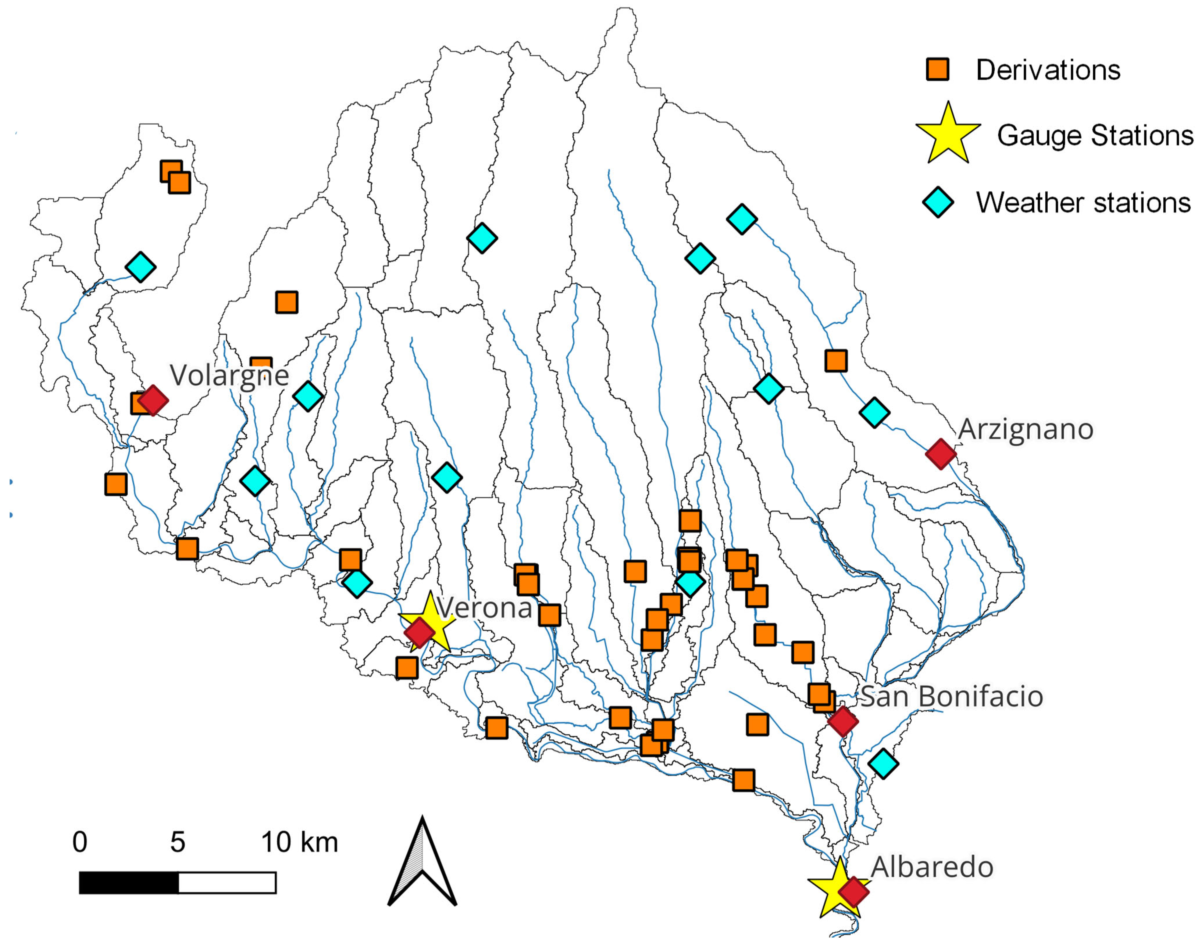
This study presents a SWAT-based hydrological model for the Adige River Lowland Basin (ARLB), a complex, flat, urbanized, and agriculturally intensive area in northeastern Italy (Figure 1). The Adige is a major contributor of nutrients to the Adriatic Sea [30], and the ARLB is one of the most economically significant areas of Europe. The model was developed to provide local administrations with a decision-supporting tool capable of simulating best management practices (BMPs) aimed at reducing nutrient loadings to the sea.
This manuscript has two main objectives. The first objective is to describe the challenges and solutions encountered while modeling a watershed of high complexity. By documenting this case study, we aim to offer a general and transferable modeling framework that can be applied to other flat, human-managed basins. Specifically, this work seeks to assist future efforts in developing tools for climate-resilient water and nutrient management in vulnerable systems, especially those in the Mediterranean region. The complexity of the terrain and the extensive artificial water network make this area a representative test case for evaluating the applicability of SWAT under such demanding conditions. The model integrates detailed crop management data and existing monitoring records for calibration and is extended to simulate nutrient transport under future climate scenarios, using three statistically downscaled regional climate models (RCMs) for two global warming levels (GWL = 2 °C and GWL = 3 °C).
The second objective is to document the first SWAT model developed for simulating nutrient transport from the ARLB. To our knowledge, this represents the first high-resolution, process-based SWAT application specifically focused on this important region of Italy. Unlike previous studies in nearby areas [27,31,32], this work incorporates detailed spatially and temporally variable agricultural management data and point-source discharges. As such, the model can be used to identify areas with the greatest impact on the main branch of the Adige River, including local tributaries or point sources with the highest nutrient loading.

2. Materials and Methods

2.1. Study Area

Adige (in Italian; Etsch in German) is the second largest river in Italy by discharge volume, with an average flow rate of approximately 190 m3/s in its lower reaches. It originates near Lake Resia in the Eastern Alps and extends for 409 km before flowing into the Adriatic Sea. The total drainage area covers 12,100 km2, mostly in the mountainous area of the Trentino–Alto–Adige region. Between Trento and Verona, it enters the Padana Plain. At Albaredo (Verona Province) is located the closing section of this study, since from there to the sea the Adige River flows 110 km more without receiving other significant contributions.
The Adige River plays a critical role in the Mediterranean hydrological and ecological systems, serving as a major source of nutrient input to the northern Adriatic Sea [30,33,34]. This study focuses exclusively on the Adige River Lowland Basin (ARLB), which extends from Volargne to Albaredo. Although the ARLB constitutes only about 1220 km2 of the entire Adige basin [33], it represents a hotspot for potential river contamination sources. The ARLB is significantly more densely populated than the rest of the basin, encompassing the city of Verona and its province, with a population of approximately 930,000. The ARLB is also more heavily modified by human activity than the upper basin, with multiple point sources along the Adige River and its tributaries (Figure 1b) and intense agricultural activity (e.g., for wine production).
Climatic conditions in the Adige basin are strongly structured by altitudinal gradients, promoting a transition from sub-Mediterranean conditions in the lower Adige valley to continental and alpine climates with increasing elevation. Mean annual temperatures in the valley descend from approximately 12–15 °C, with notable seasonal extremes (winter minima near 0 °C and summer maxima exceeding 30 °C) [35,36].
The Adige River Basin is generally characterized by cold winters and peak precipitation occurring predominantly in the summer months. At higher elevations, substantial amounts of snow accumulate during winter, serving as a key water reserve that is progressively released through snowmelt beginning in spring. This dynamic gives rise to a nival hydrological regime, marked by high water availability during the warm season and low flows during winter. Annual precipitation totals are relatively high, but their distribution varies significantly with elevation, valley orientation, and proximity to the outer margins of the Alpine chain. Precipitation ranges from 400 to 500 mm/year in sheltered and lower areas to up to 1600 mm/year in high-altitude zones or valleys exposed toward the Po Plain [33,36].
Recent research on climate change effects in the Adige River Basin showed increased temperature and altered precipitation patterns, resulting in declining summer runoff (−13% since 1957) and increasing winter flow (+30%), with glacier retreat (~2.3 km2/year) further altering baseflow contributions [37]. Recent extreme climate events, such as the remarkably warm and dry heatwave of May 2022, highlight the basin’s increased vulnerability to aggravated hydroclimatic stress.

2.2. Data Availability and Modeling Approach

We simulated flow and nutrient transport in the ARLB using SWAT. Theoretical aspects of this widely adopted code, including the subroutines used to calculate overland flow, nutrient transport, and routing through streams, can be found in several reviews and books [3]. A comprehensive SWAT documentation can be found at https://swat.tamu.edu/docs/ (accessed on 29 August 2025). Briefly, SWAT divides a basin into multiple subbasins, which are further subdivided into hydrological response units (HRUs) with homogeneous land use, topography, and soil characteristics (consequently, also homogeneous management). Using a combination of meteorological data, soil and land use properties, along with input from point and diffuse sources, SWAT calculates the components of the flow budget (evapotranspiration, runoff, storage, and infiltration). A similar procedure is used to compute the nutrient mass balance.
The SWAT model was developed following established workflows to simulate climate change scenarios [3,16]. First, we discretized and parameterized the study area and calibrated a reference (“present-day”) model. We then modified the present-day model to account for the impact of climate change, making predictions of “future” streamflow and nutrient loadings, which were subsequently compared with present-day conditions. To increase its transferability, the model was developed exclusively using open-source codes. Specifically, we used SWAT2012 v.664, the QGIS plugin QSWAT v3_12, and several custom Python v.3.12 and R v.4.5.1 scripts to facilitate model pre- and post-processing.
The present-day model simulated the period from 2001 to 2020. The first seven years (2001–2007) were used for model warm-up, while the remaining years (2008–2020) were used for reference results. SWAT calculations adopt daily timesteps, and their results were lumped using a monthly approach. Reaches and subbasins were created using the D8 algorithm of the code TauDEM [38], integrated with QSWAT, using as a topographic base the ASTER digital elevation model (DEM), with a resolution of 30 m × 30 m [39].

2.3. Challenge #1: Creation of Reaches in Flat Terrain

The creation of reaches and subbasins was challenged by two primary factors. The first difficulty was that the study area is predominantly flat, with only a few local slopes exceeding 10%. This flat terrain complicates hydrological modeling, as evidenced by the difficulties encountered when configuring the river network using TauDEM. To address this issue, we “burnt-in” a vector file representing the main streams, based on the official river basin management plan [40], ensuring that TauDEM generated a river network that aligned with the actual distribution of streams. The burning technique is a common method in flow enforcement that modifies the DEM by creating new channels that guide the flow algorithms, ensuring the resulting drainage patterns match the mapped hydrography [41,42]. After initial trials, a 10 km2 drainage area threshold in TauDEM was applied to generate flow segments and a reasonable number of subbasins to ensure computational efficiency while keeping sufficient spatial variability and accuracy.
The second difficulty was that the Adige lowland area is characterized by a complex network of human-altered streams. Some of these canals can have a strong impact on the water budget; for instance, the “Canale Biffis”, a manmade canal that feeds a run-of-the-river (ROR) hydroelectric power station near Volargne. The canal has a maximum discharge flow of about 135 m3/s. It extracts water from the Adige River near the municipality of Ala (upstream of the modeled area) and returns it to the Chievo dam near the city of Verona. In addition to the Canale Biffis, a vast network of secondary canals exists, some of which are oriented against the topographic gradients calculated by TauDEM. Counter-gradient stream routing cannot be simulated in SWAT. A Further difficulty when reproducing them with SWAT is that streams from a single channel cannot be parted into two or more tributaries, which occur, for example, at bypass points of the artificial channels.
To address these challenges, we manually modified the river network by simplifying it and eliminating counter-gradient streams. In line with other SWAT-based studies on human-altered stream networks [43,44], we replaced diversions and artificial canals (Figure 2) with point sources, which were added to each subbasin to account for the water balance of multiple diversions and releases, including those from industrial and sewage treatment plants. Discharge data for diversions and releases from major irrigation canals were provided by the National Drainage and Irrigation Association (ANBI) and ROR hydroelectric plant managers. The comparison between the original and modified stream network is provided in Figure S1 (Supplementary Material), showing also the final stream network produced by SWAT on which the outputs of the simulations are calculated.

2.4. Challenge #2: Limited Weather Data

Weather data were provided by the local meteorological agency and included daily data on precipitation, solar radiation, humidity, wind speed, and temperature from multiple stations (Figure 2). Since SWAT requires weather data for all subbasins, we used an inverse distance weighting (IDW) interpolation method to estimate data for subbasins without stations. Tuo et al. [45] concluded that IDW outperformed other algorithms in helping SWAT models match observed streamflow discharge. Similarly, Camera et al. [46] found that the IDW was one of the best methods for interpolating local daily weather data.

2.5. Challenge #3: Soil Type and Land Use Heterogeneity

Soil types and corresponding hydrological properties and parameters (e.g., Available Water Capacity (AWC), saturated hydraulic conductivity (K), and Runoff Curve Number (CN)) were obtained from the regional environmental agency of Veneto (ARPAV) [47], covering the entire lowland area. For the few mountain areas not covered by the ARPAV map, missing data were sourced from the Harmonized World Soil Database (HWSD) [48]. A table with the conversion between HWSD maps and SWAT entries is provided in the Supplementary Material (Table S1), along with a map of dominant soil types in the subbasins (Figure S2).
Diffuse sources were integrated into the SWAT model to capture spatial and temporal variability in nutrient transport due to agriculture. We first generated a land use map based on the Corine Land Cover 2018 (CLC2018) and the EUCROP 2018 dataset [49]. The EUCROP map (10 × 10 m resolution) was reclassified to match the 30 × 30 m grid size of the SWAT hydrological response units (HRUs). For the coarser-grid CLC map (100 × 100 m), values were extracted at each SWAT grid cell center. A map of dominant land uses across subbasins is included in the Supplementary Material (Figure S3).

2.6. Challenge #4: Use of Detailed Agricultural Practices

Fertilizer types, dosages, and application timings for major crops in the Adige lowland were provided by the Veneto regional authority (“Direzione Agroambiente, programmazione e gestione ittica e faunistico venatoria”), based on best management practices, technical manuals, and existing regulations (Table 1). Nitrogen application rates conform to the regional Nitrates Action Programme, implemented under Directive 91/676/EEC and its national transposition. Crop types considered in this work were maize (Zea mays L.), wheat (Triticum Aestivum L.), barley (Hordeum vulgare L.), soybean (Glycine max L.), sunflower (Heliantus annuus L.), rapeseed (Brassica napus L.), potato (Solanum tuberosum L.), sugar beet (Beta vulgaris L.), vineyards, olive groves, apple orchards, pastures and meadows, representative of regional agricultural patterns [50]. A correspondence table between crop types and SWAT classes is provided in the Supplementary Material (Table S2). The dataset includes fertilizer type (organic or mineral), application date, and dosage (kg/ha), with fertilizer IDs matching those in the SWAT database (available online: https://swat.tamu.edu/media/69419/Appendix-A.pdf, Appendix A.4; accessed on 9 September 2025). As spatial data on fertilizer types were unavailable, a weighted average was used to combine mineral and organic inputs, with percentages reported in Table 1. Following the previous SWAT-based approach [51], elemental nitrogen (N, kg/ha) and elemental phosphorus (P, kg/ha) were calculated per crop (Table 1). For example, for barley, a typical application of 300 kg/ha of inorganic fertilizer (06-24-24, containing 6% N and 24% P) in October results in 18 kg N/ha and 31 kg P/ha being input into the model, assuming a 40% effective application rate. When applicable, sowing and harvest dates were also provided by the regional authority.

2.7. Challenge #5: Multiple Point Sources

Point sources were used to account for the industrial and WWTP discharges within each subbasin, in terms of flow and nutrient mass (Figure 1b). Such flow was then summed to the net discharge rate obtained from the water balance of multiple diversions and releases, as abovementioned. SWAT can accept either constant or daily variable loads (kg/day) for different N species (e.g., nitrate, ammonia) and phosphorus (as phosphate). While daily variable loads would better capture seasonal changes in point source discharges, such as increased summer discharges due to tourism, our monitoring data were insufficient to support such a calculation. The data, collected bi-weekly or less frequently between 2008 and 2020, contained gaps and lacked consistency. Other gaps were that only annual average flow rates were available (Figure 1b), and our simulations began in 2001. Due to these limitations, we used constant average loads for each point source, calculated by multiplying the average annual nutrient concentrations (e.g., nitrate, ammonia, phosphate) by the annual average discharge flow.
A special point source (“inlet”) was included to simulate incoming water flow and nutrient loadings from the upstream Adige basin. Flow data were taken from the Vo’ Destro gauge station, which provided continuous measurements for 2001–2020, with less than 5% missing data, filled by linear interpolation. Since the nutrient concentration time series at this gauge station was largely incomplete, constant average values for nitrogen and phosphorus species were used. We also noticed that most available phosphorus measurements were below the detection limit (<0.04 mg/L). Setting total phosphorus (TP) to zero was considered inappropriate, since the upstream Adige River is impacted by various chemical stressors [33] that may contribute to phosphorus loadings. As such, we used a reference TP concentration of 0.015 mg/L, which is based on average reactive phosphorus levels measured near Rovereto from March to September 2008 [52].

2.8. Calibration and Validation

To ensure model accuracy and reliability, we performed calibration and validation following established guidelines [53]. Our approach did not follow a conventional 70:30 split for calibration and validation. This was a deliberate decision, as applying such a split would have resulted in an insufficient number of data points for the validation period, reducing its statistical significance. Instead, we adopted a functional separation, such that streamflow data were used for calibration, and nutrient concentration data were used for validation, recognizing that nutrient transport is generally more challenging to model than flow.
Calibration was based on streamflow matching [3] using the SWAT-CUP tool [54] to compare monthly simulated and observed streamflow data at two most reliable monitoring stations on the Adige River, one close to Albaredo (“Adige–Albaredo”) and one close to Verona (“Adige–Verona”). The reference data were obtained from the regional environmental agency (ARPAV). Details regarding the streamflow measurements can be found in technical documents available at the ARPAV website https://www.arpa.veneto.it; accessed on 29 August 2025. Table 2 lists the 16 SWAT parameters that we chose from the range of possible SWAT parameters and adjusted during calibration. We selected these parameters according to previous SWAT-CUP calibrations using SUFI-2. A total of 500 simulations were carried out. Parameter ranges (bounded by minimum and maximum values) are shown in the table. Parameters labeled with “r” (relative variation) were multiplied by 1 ± x r , where x r is a random number within the range. A random substitution was performed on the parameters labeled with “v” (replace), meaning the existing parameter value is to be replaced by a random value   x v within the range.
Best-fit parameters were obtained by minimizing the difference between observed and simulated data [3,53]. We first focused on the Nash–Sutcliffe Efficiency (NSE), possibly the most widely adopted metric, defined as
N S E = 1 i = 1 N ( Q i s i m Q i o b s ) i = 1 N ( Q i s i m Q ¯ o b s )
and ranging from –∞ to 1.0, with values between 0.0 and 1.0 indicating acceptable model performance. A negative NSE suggests poor performance, where the observed mean is a better predictor than the model [53]. Notice that SWAT-CUP produces several other metrics that could also be used to measure model calibration and validation. Among them, we highlighted the PBIAS, which measures the average tendency of the model to over- or under-predict, and which is often preferred over other metrics to examine the model validation quality [55]. A value of 0.0 is ideal. Positive PBIAS indicates the model underestimates, while negative values suggest overestimation [56]. The formula of the PBIAS is
P B I A S = i = 1 N ( Q i s i m Q i o b s ) i = 1 N ( Q i o b s )
To validate the calibrated model, we first compared the total nitrogen (TN) concentrations at the “Adige–Albaredo” monitoring station calculated using SWAT (without further calibration) against the observations at the same station. As for the streamflow data, this represents the most complete and reliable dataset existing for validating purposes. Available measurement data were collected between 2013 and 2020. Then, we compared the year-averaged TN loadings in other existing water quality monitoring in the basin to assess if the model can capture the intra-subbasins variability in terms of nutrient loadings. Since all monitoring points (except “Adige–Verona” and “Adige–Albaredo”) lacked measured streamflow rates, we used the SWAT-calculated flows to compute the loadings.

2.9. Climate Change Scenarios

Climate change scenarios were developed for SWAT using the SSP5-8.5 forcing pathway [21] at two Global Warming Levels (GWLs), at 2 °C and at 3 °C (Table 3). These GWLs align with the targets of the Paris Agreement, which has shifted focus from emission scenarios to global warming levels when assessing climate impacts [57]. To address uncertainty in climate projections, we used three versions of the RegCM4-6 regional climate model (RCM), each driven by a different Global Circulation Model (GCM), produced by the Abdus Salam International Centre for Theoretical Physics (Trieste, Italy). These simulations, covering the EUR-11 domain, were obtained from the Earth System Grid Federation (ESGF) and are part of the CORDEX initiative [58]. Time series for key climate variables (precipitation, temperature, humidity, wind) were statistically downscaled for each subbasin using a Monthly Quantile Delta Mapping (QDM) approach [59,60,61]. The baseline period for downscaling was 2001–2020, matching the ARPAV weather data. For ratio-based variables, thresholds were set as 0.2 mm for precipitation, 0.1 m/s for wind, and 0.02 for humidity. The GWL scenarios were implemented in SWAT by replacing reference (present-day) weather data with the downscaled future projections for each scenario (Table 3). The model setup remained the same as the reference simulation, including the 20-year run and 7-year spin-up.

2.10. Evaluation Metrics

The model results were analyzed by looking at maps and time series for three key variables: (a) flow rates (Q), (b) total nitrogen (TN), and (c) total phosphorus (TP). One set of maps showed the average yearly Q, TN, and TP levels in the main water bodies under current conditions. This helped assess the current impact of nutrients on the streams, including the main Adige River and its tributaries. Another set of maps showed the influence of diffuse pollution sources in different subbasins. These maps displayed the amount of TN or TP entering water bodies, adjusted for the size of each subbasin (in kg/ha). This was performed for both current conditions and future climate scenarios, and the differences were compared.
Time series were also used to track Q, TN, and TP passing through the “Adige-Albaredo” gauge station, which is located at the end of the watershed and thus represents what eventually reaches the Mediterranean Sea. First, data for the current situation were shown. Then, the difference ( Δ ) between future climate scenarios and the reference model was calculated. For instance, for flow, the difference Δ Q was computed as
Δ Q ( i ) = Q c c ( i ) Q r e f ( i )
where i is the progressive number of the month since time zero (i = 1, …, 156). Finally, we calculated the cumulative monthly difference. For instance, for flow, this resulted as
Q c u m ( i ) = i Q c c ( i ) Q r e f ( i )
Cumulative values emphasize trends of the impact of climate change. For instance, they may suggest whether the Adige River is expected to increase or decrease its nutrient transport over a predefined period in the future.

3. Results

3.1. Calibration and Validation

The SWAT model resulted in 73 subbasins, encompassing a total area of 121,974.12 hectares (or 1219.74 km2). The boundaries of these subbasins are illustrated in Figure 1b (black lines). Their areal extension is quite variable across the subbasins, ranging from 0.36 ha to 11,252.88 ha. The smallest subbasins are located downstream of the municipality of Albaredo, where the river is artificially channeled and disconnected from the surrounding land.
A strong agreement was observed between measured and simulated streamflow rates (Q), indicating that the model calibration was successfully achieved. Figure 3a presents a visual comparison of observed and simulated Q at the “Adige–Albaredo” station. The best-fit simulation (red line) closely follows the observed data (blue line), confirming the model accuracy. This is further supported by a Nash–Sutcliffe Efficiency (NSE) value of 0.76 at the “Adige–Verona” station, i.e., a “very good” performance [53]. The corresponding Percent Bias (PBIAS) at “Adige–Albaredo” was 12.00%, also indicating a satisfactory calibration. Comparable results were obtained at the “Adige–Verona” station, where the NSE reached 0.69, rated as “good,” and the PBIAS was −11.80%. A complete summary of calibration statistics generated by SWAT-CUP is provided in Table 4.
A satisfactory model validation was also obtained. Figure 3b indicates that the model effectively captured the observed total nitrogen (TN) loadings at the “Adige–Albaredo” monitoring point. The simulated mean (year-round) concentration was 1.08 mg/L, which closely matched an observed mean concentration of 1.09 mg/L. The validation yielded an NSE of 0.07 and a PBIAS of 0.77 % . These values were considered acceptable given the inherently higher uncertainty in simulating nutrient transport compared to streamflow. Moreover, we considered that the PBIAS offers a more favorable assessment of model performance than the NSE, which can be attributed to the NSE’s sensitivity to various factors, such as sample size or the irregular intervals between observations [62,63], all of which may influence our dataset.
The limited sample size may also explain why statistical outliers do not significantly alter the NSE, as evaluated by removing the highest residuals between simulated and calculated values (Figure S4; Supplementary Material). Furthermore, the measured water quality data represent specific sampling days, whereas the model outputs represent average monthly concentrations, potentially smoothing short-term variability. This may also explain why the correlation between simulated and observed values was around 0.40 (i.e., a weak-to-moderate positive linear relationship), while the normalized standard deviation (standard deviation of the simulated values divided by that of the observation) was 0.45 (see the Taylor diagram reported in Figure S4; Supplementary Material). Nevertheless, the model remains suitable for the purpose of this study, which centers on long-term mass balance rather than daily scale accuracy.
The comparison between calculated and observed annual TN loadings indicates that the model catches the spatial variability of loadings across the subbasins. The results (Figure 3c) indicate a nice correspondence between predicted and calculated loadings, with a root mean square error (RMSE) of 0.13. Note that the best-fit linear trend between simulated and reference loadings had a slope of 0.87, which means that, on average, the model underpredicts the measured loadings by 13%. This error was deemed acceptable, recalling that these predictions were run without further model calibration to avoid model overfitting. We also recall that the reference loadings were obtained using the SWAT-predicted streamflow rates from ungauged catchments, which may induce uncertainty in the validation targets.

3.2. Streamflow Simulations

The calibrated SWAT model simulated an average Adige River discharge over the 2008–2020 period close to Q = 192 m3/s, which is similar to the observed values for the same period ( Q = 218 m3/s) (Table 4). The model is able to capture the intra-seasonal fluctuations, as visually appreciated by the hydrographs at “Adige–Albaredo” reported in Figure 3a and by a similar standard deviation ( σ ) of the streamflow rates (simulated σ = 106 m3/s; observed σ = 100 m3/s). The model is also able to capture the highest discharge peaks (monthly averaged Q > 200 m3/s) occurring in spring (February to April) due to snowmelt from the Alps [33]. Smaller peaks observed in autumn (September to November) are due to rainfall events. The model slightly underestimates the baseflow, which is lowest in the summer (June to September), with Q = 100 m3/s. We accepted this error, considering the simplification introduced to the model compared to the more complex reality and the inherent error associated with the streamflow measurements.
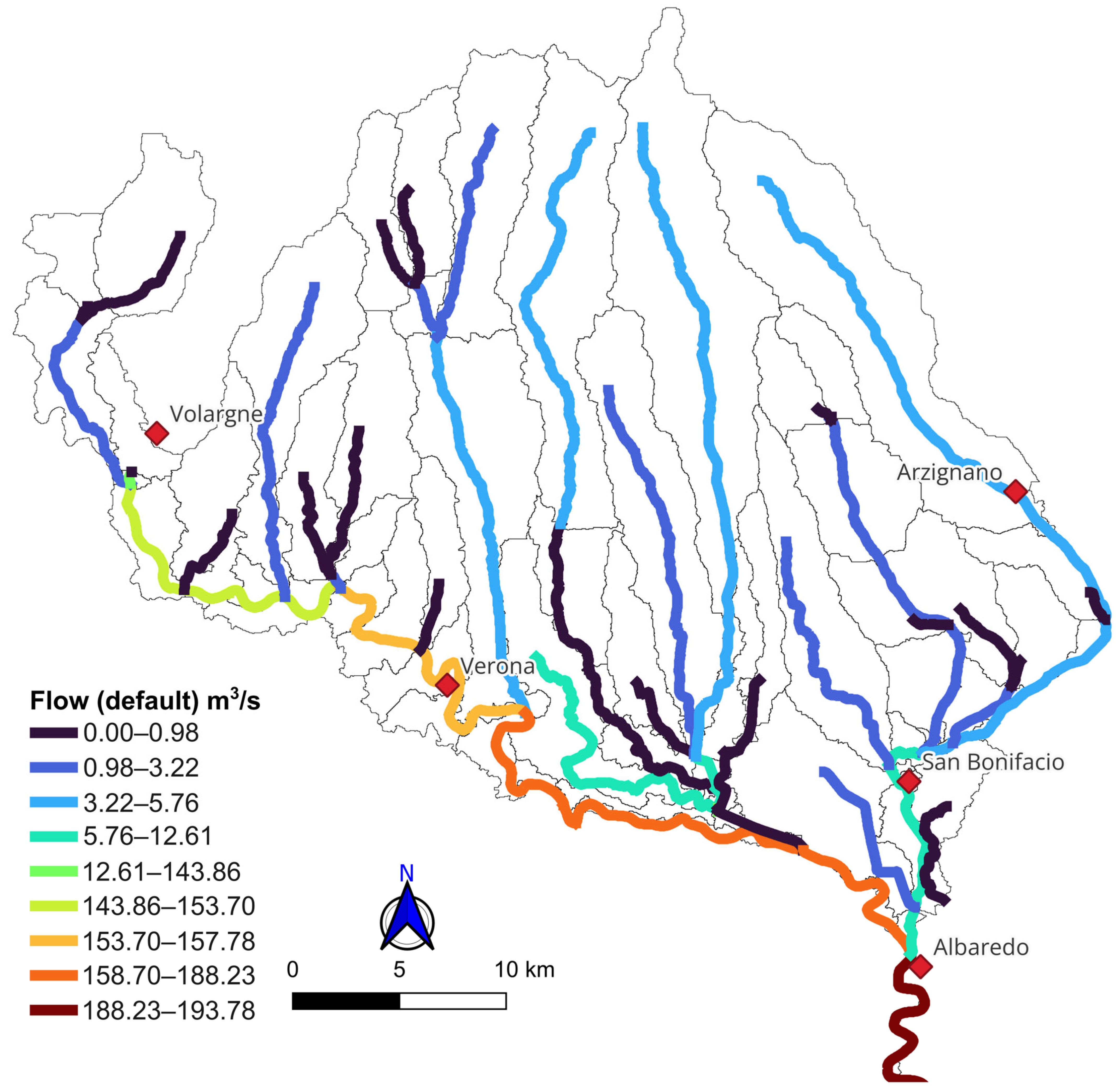
Figure 4 shows the average yearly flow rates (m3/s) in the main water bodies of the ARLB, based on the calibrated SWAT model. The values represent averages over the 13-year simulation period (2008–2020). Across the study area, the Adige River’s flow increases from about 143 m3/s at Volargne to about 192 m3/s at Albaredo, corresponding to a 35% increase. Tributaries play a limited role, with the highest average flow reaching only 13 m3/s in the Chiampo River. A notable increase in the Adige flow is due to contributions from the Biffis Canal in the proximity of Verona. Tributaries from the Lessini Mountains contribute only modestly to the total flow.
We then compared the present-day model results with those projected under climate change scenarios. Summary tables presenting monthly average values for observed (i.e., “reference”) data, control simulations from three post-bias-correction models (for the period 2001–2020), and future projections under two Global Warming Levels (GWL = 2 °C and GWL = 3 °C) are provided in the Supplementary Material (Table S3). Daily time series of precipitation, minimum and maximum temperature, wind speed, and humidity across the Adige River subbasins are also included. An example of the summary statistics is shown in Table 5, with precipitation data for the Adige River basin. Notably, the simulated control values from each climate model closely align with the reference observations, supporting the reliability of the downscaling process. Under climate change scenarios, these values show significant variation. Monthly responses vary across models, with differing trends of increase or decrease. Overall, the models consistently suggest longer and more intense dry spells during the spring–summer period (mid-March to mid-September), and a tendency toward wetter conditions in the autumn–winter months (mid-September to mid-March).
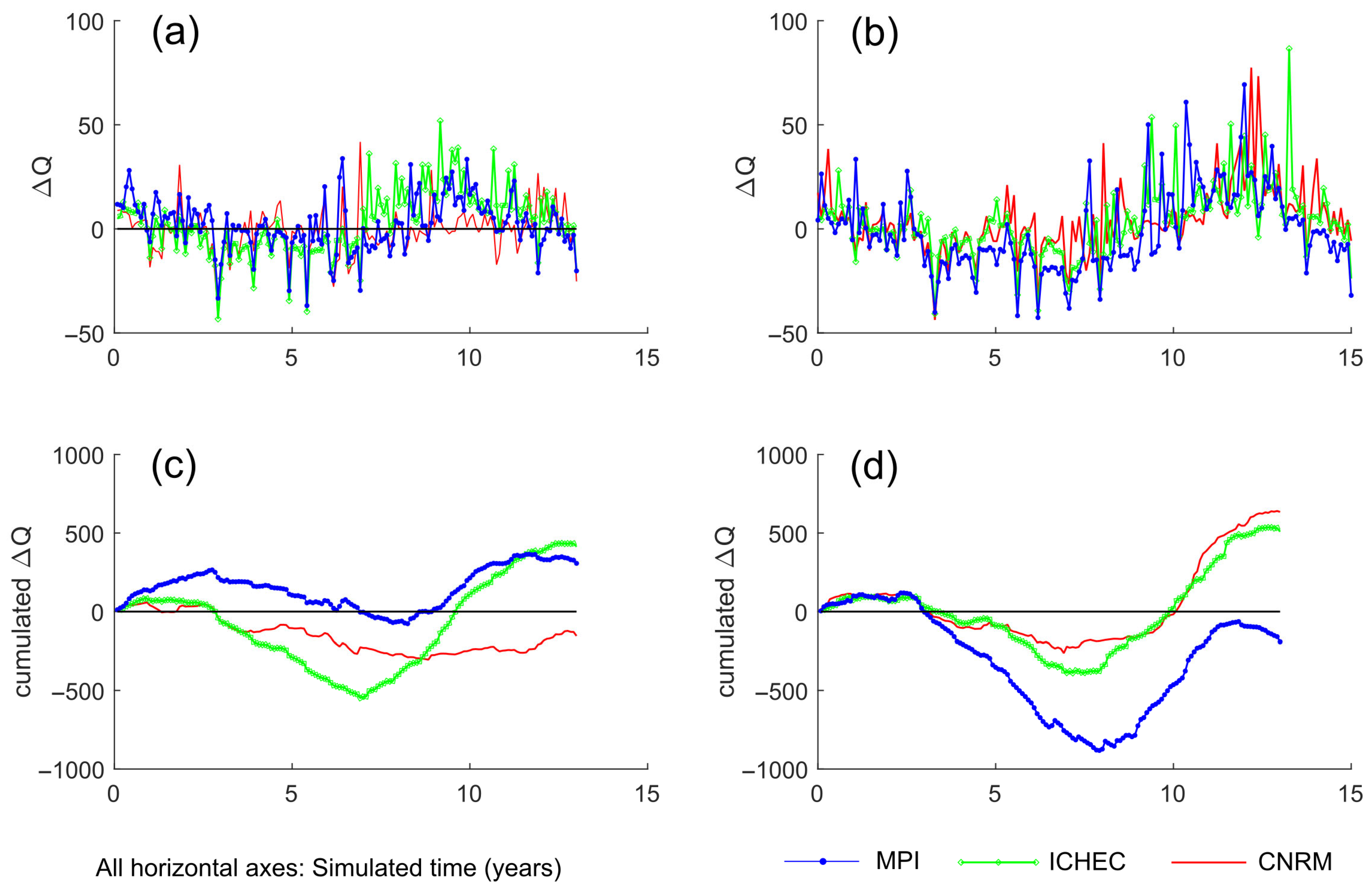
Figure 5a shows the difference in monthly averaged discharge rates ( Δ Q ) between the three climate change models ( Q ) at a global warming level (GWL) of 2 °C and the reference model ( Q r e f ) (Figure 4), such that Δ Q   =   Q     Q r e f . To compare the different scenarios on the same timeline, we set the first year of each model (Table 3) as “year zero.” The results indicate that future discharge rates differ from those in the reference period, with variations of about ±50 m3/s. Negative variations are especially important, as they can make discharge rate fall into the range of historically low flow rates, with potentially catastrophic consequences. For instance, if discharge falls below 80 m3/s for long periods, seawater could intrude up to 100 km inland, affecting the flat Polesine area, south-east of Verona [64]. Looking at Figure 5a, a repeating cycle is evident over the 13-year simulation. This may be influenced by larger climate patterns, such as the North Atlantic Oscillation (NAO), which affect the Global Circulation Models (GCMs) used here. Because of the different weather statistics, such as the precipitation (Table 5), each tested model predicts different discharge trends for the Adige River. These differences become more noticeable in the 3 °C scenario (Figure 5b). In that case, variations range from −50 m3/s to +100 m3/s, especially toward the end of the simulation. These higher peaks reflect more extreme weather conditions expected under increasing warming levels.
The cumulative differences between future discharge and the reference scenario are shown in Figure 5c,d for the 2 °C and 3 °C cases. All models show an initial increase in discharge, followed by a dip around years 6–10, and then a rise again around years 10–12. The simulation ends at year 13, so we could not assess if this cycle continues. Notice that the models behave quite differently. At 2 °C warming, ICHEC shows large fluctuations, MPI generally predicts more water flow than the reference, while CNRM shows less flow than the reference. At 3 °C warming, ICHEC and CNRM behave similarly to their 2 °C patterns, while MPI shows a more dramatic drop in cumulative discharge during the middle years.

3.3. Nutrient Simulations

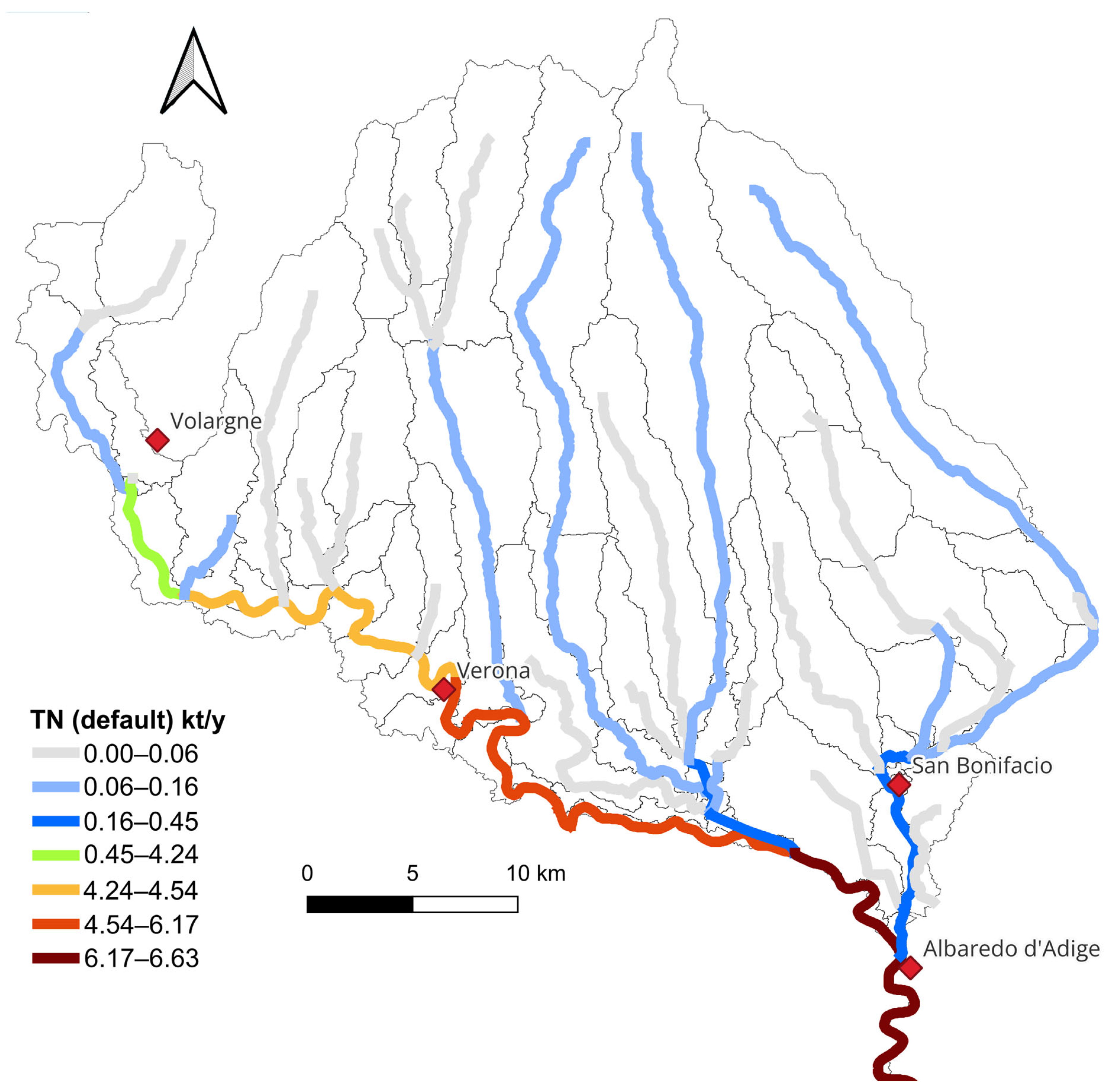
Well-defined patterns emerge in nitrogen transport dynamics from the present-day and climate-change SWAT simulations. Figure 6 shows the current average annual total nitrogen (TN) loadings, expressed in kilotons per year (kt/y), in the main water bodies of the ARLB. A progressive increase along the Adige River is clearly visible. The relative increase from the inlet at Volargne (loadings close to 4.2 kt/y) to the Albaredo gauge station (6.6 kt/y) is +57%, which is higher than the relative increase in flow rates occurring (+35%) for the same river course. This means that loadings are due to both an increase in flow rates and TN mass (i.e., TN concentration) entering the Adige River in the lowland area.
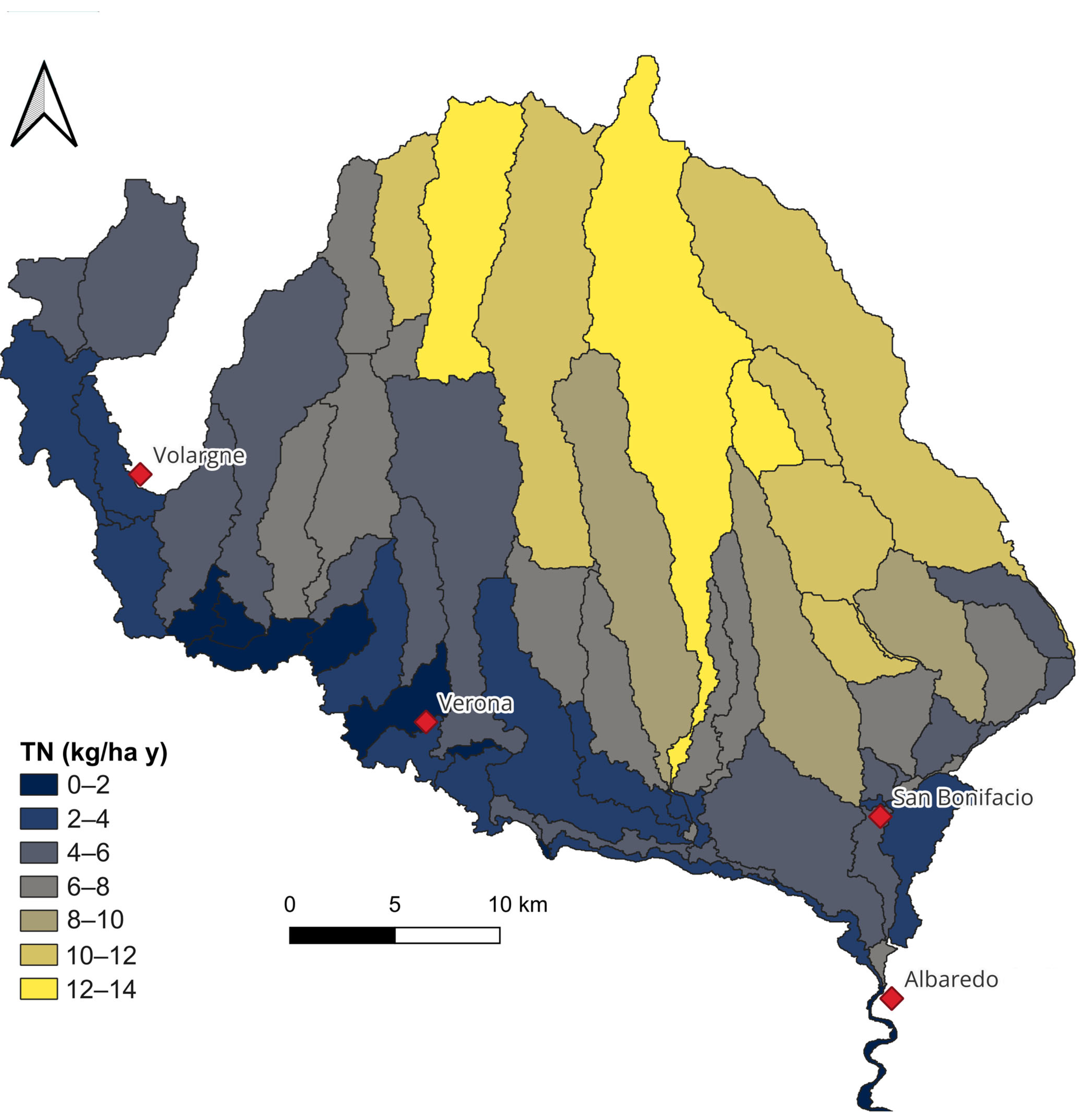
This increase in TN loadings along the Adige River is a consequence of the strong spatial variability of all TN sources, associated with both diffuse and point sources. In Figure 6, the contribution of pre-Alpine subbasins included in the modeling domain is well distinguished. The loading from these subbasins depends directly on the agricultural practices across the basins, which create nutrient sources that eventually enter the Adige tributaries. Figure 7 illustrates the average annual TN input from diffuse sources (mainly agricultural runoff) across the various subbasins, normalized by area (expressed in kg/ha). This spatial distribution highlights the areas within the Adige River Lake Basin (ARLB) that contribute most significantly to diffuse nitrogen pollution. In particular, the hilly subbasins in the northern part of the study area exhibit the highest values, with peak contributions ranging from 12 to 14 kg/ha.
The visual assessment of Figure 6 suggests that the contribution of Adige River tributaries from the Pre-Alpine subbasins is more limited than the impact of point sources located along the main course of the Adige River. For example, there is a noticeable increase in nitrogen load near Verona, which can be attributed to the basin’s largest wastewater treatment plant (WWTP). This facility has an average nitrogen concentration of approximately 13 mg/L and a discharge rate of about 77,000 m3/day. As a result, it contributes around 1000 kg/day of total nitrogen (TN), equivalent to roughly 365 t TN/y solely from this point source. For comparison, the Chiampo River contributes approximately 400 t TN/y at its confluence with the Adige near Albaredo. The Chiampo River is also partially influenced by the second-largest WWTP in the basin, located near San Bonifacio, which discharges around 26 tons of TN per year.
A more quantitative evaluation supporting the conclusion that point sources have a greater influence than diffuse sources on the overall nutrient budget was obtained using the “SWAT Check” tool embedded in QSWAT. According to this tool, at the scale of the ARLB, the impact of point sources, averaged over the 13-year simulation period, accounts for approximately 65% (2.1 kt/y) of the total TN budget (3.4 kt/y).
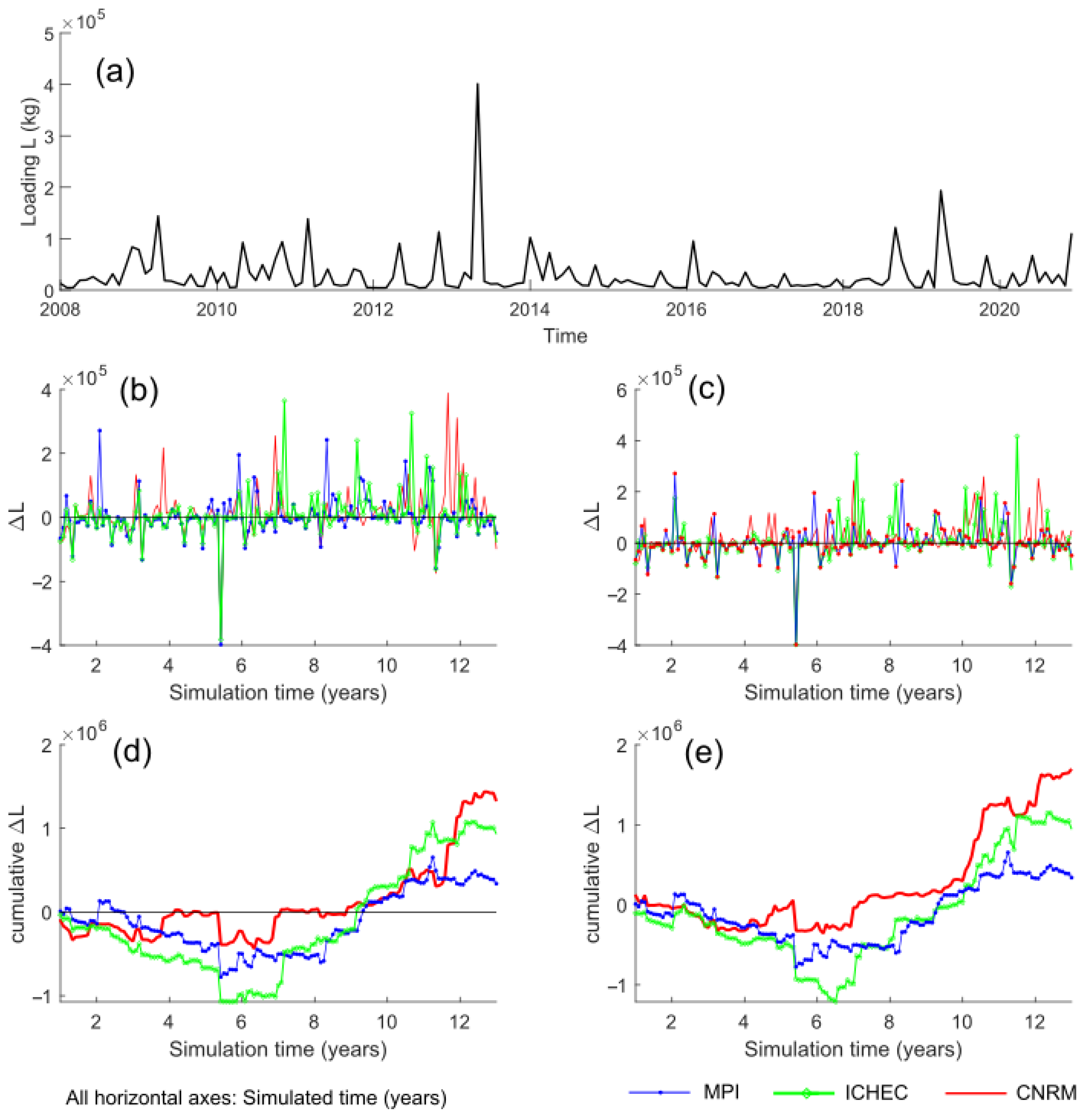
Seasonal variability in precipitation and temperature was found to significantly influence the modeled dynamics of nutrient transport. Figure 8a displays the time series of simulated TN loadings across the main water bodies. Consistent with the patterns observed in flow rates (Figure 5), notable discrepancies emerge between the present-day scenario and projections under future climate scenarios, as depicted in Figure 8b,c, corresponding to global warming levels (GWL) of 2 °C and 3 °C, respectively.
The cumulative differences between scenarios underscore the role of hydrological seasonality in shaping TN loading trends. For example, under the GWL = 2 °C scenario (Figure 8d), the ICHEC-driven climate simulation produced the most pronounced reduction in TN loadings during simulation years 6 to 8, aligning with a concurrent decline in cumulative flow rates reported in Figure 5. This suggests a strong coupling between flow dynamics and nutrient transport under changing climatic conditions for 2 °C and 3 °C temperature change, respectively.
Figure 8d,e show that, overall, all climate models predict a long-term increase in cumulative total nitrogen (TN) loadings under both global warming scenarios. In the GWL = 2 °C scenario (Figure 8d), TN loadings are projected to rise by approximately 2000 tons over the 13-year simulation period (about 150 tons per year). Under the GWL = 3 °C scenario (Figure 8e), the increase is projected to rise to about 300 tons per year, i.e., to double the previous result.
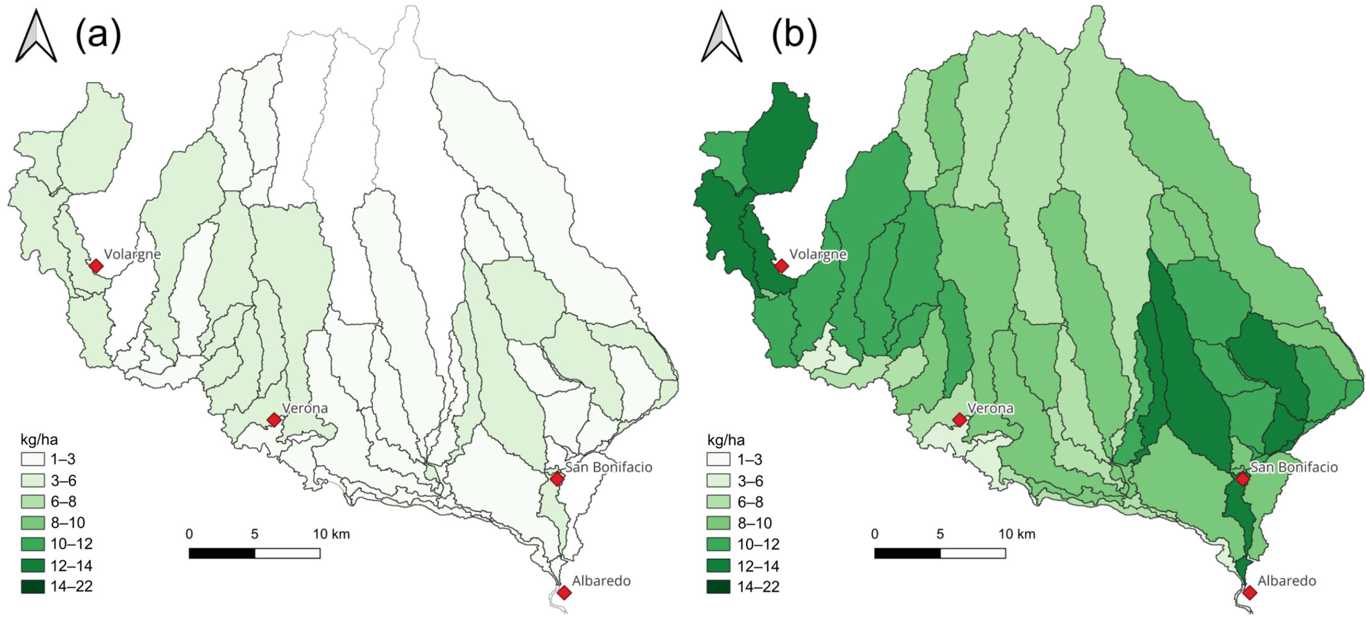
To assess the impact of climate change on the spatial distribution of TN, we mapped the difference in TN loadings between climate-change-adjusted models and the baseline scenario. Two examples are presented in Figure 9a,b. The complete set of results for all simulated scenarios is provided in the Supplementary Material (Figures S5–S10). In these figures, positive values indicate an increase in nitrogen mass produced in a subbasin relative to the reference model. Figure 9a shows the results for the CNRM-driven simulation under the GWL = 2 °C scenario. Here, all values are positive, indicating a consistent increase in TN loadings across all subbasins compared to the reference. The highest increases fall within the range of 6–8 kg/ha. Figure 9b presents the results for the MPI-driven simulation under the GWL = 3 °C scenario. In this case, the differences in TN loadings are significantly larger than those observed in the CNRM-2 °C scenario. In several subbasins, increases exceed 10 kg/ha, with the maximum reaching up to 22 kg/ha.
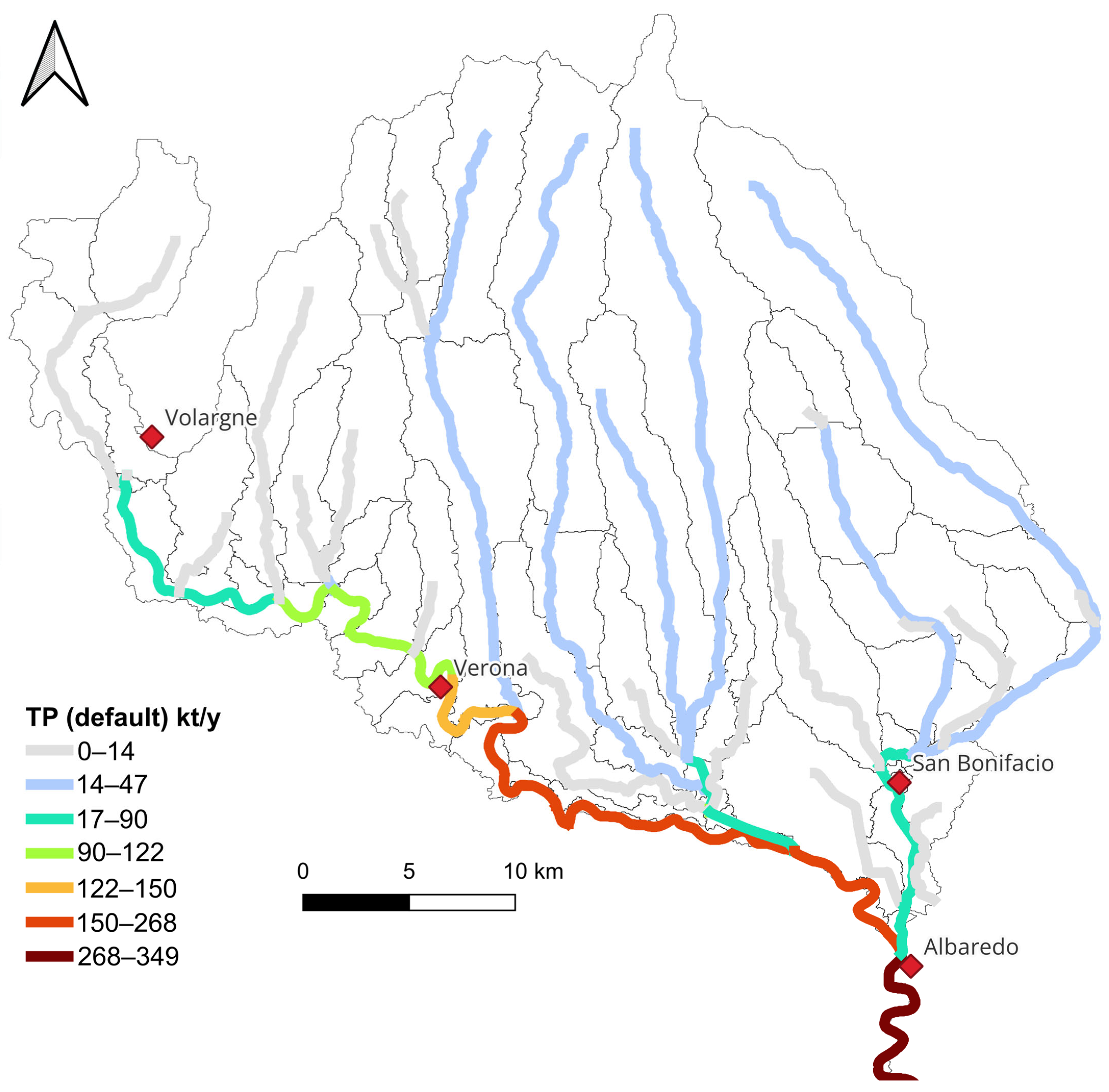
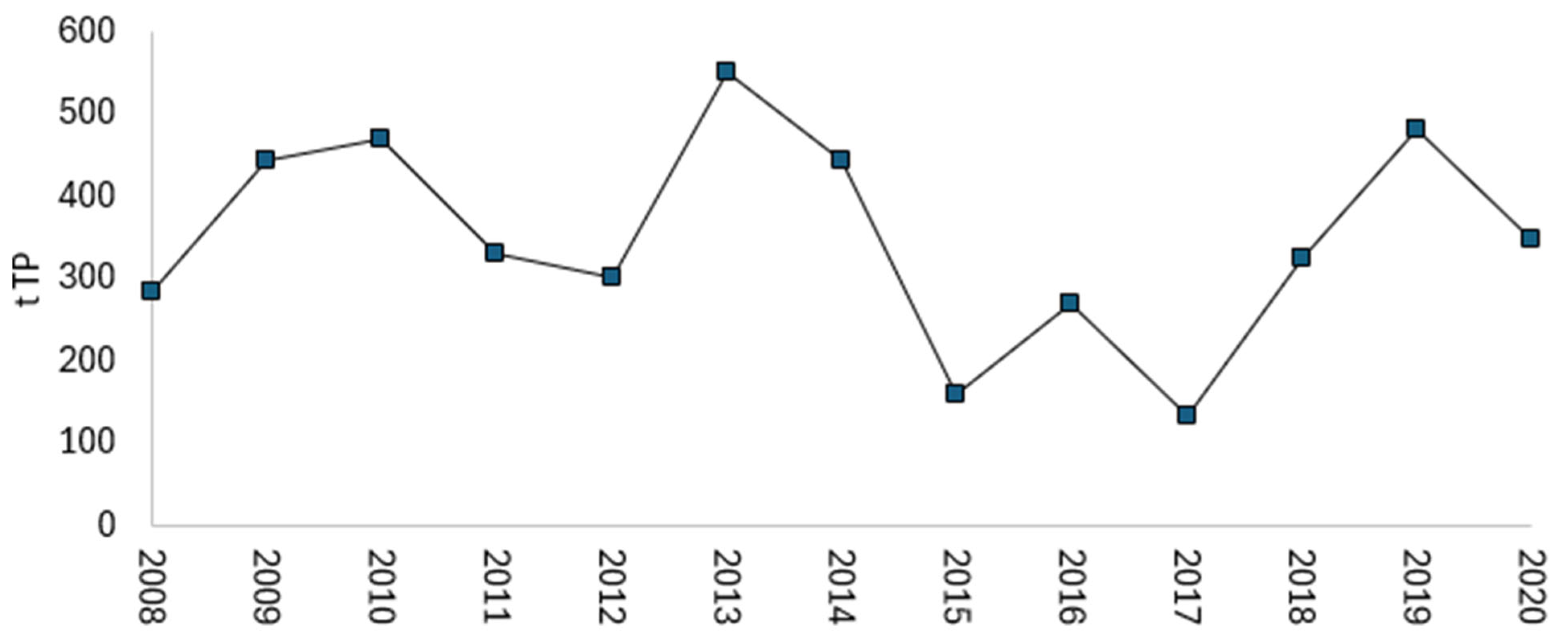
A similar analysis was conducted to analyze phosphorus transport under present-day and future conditions, with different results. Figure 10 illustrates the current average annual total phosphorus (TP) loadings in the main ARLB streams. While TP loadings are generally lower than TN loadings, their spatial distribution across streams closely mirrors the patterns previously described for TN (Figure 6). A key distinction between TN and TP lies in the magnitude of the increase observed along the Adige River. At the inlet near Volargne, TP loadings are approximately 50 tons/y, rising sharply to about 350 tons/y at the outlet near Albaredo. This represents a 700% increase as the river crosses the lowland area, which is substantially higher than the 57% increase reported for TN in the same section, as discussed previously.
Other distinctions compared to the analysis of TN were found from the time series analysis of present-day and future scenarios. Figure 11a presents the time series of simulated total phosphorus (TP) loadings in the main water bodies. As observed in the corresponding analysis for TN (Figure 8), notable differences emerge between projections from the climate change scenarios and the present-day model. These differences are shown in Figure 11b,c for GWL = 2 °C and GWL = 3 °C, respectively. Seasonal variations in flow continue to influence TP loadings across all tested GCMs and warming scenarios. While cumulative TP loadings vary considerably among the three GCMs by the end of the 13-year simulation period, the differences between the two warming levels are less pronounced (contrary to what was observed for TN). Under the GWL = 2 °C scenario (Figure 11d), the CNRM-driven RCM projects an increase in TP loadings of approximately 1200 tons over the simulation period, corresponding to an average annual increase of about 92 tons. A comparable increase is predicted for the GWL = 3 °C scenario (Figure 11e). In contrast, the MPI-driven RCM estimates a more modest rise of around 400 tons over 13 years under both GWL scenarios, equating to an average of approximately 30 tons/y.
The different impact of the global warming levels on TP compared to TN can also be appreciated from the variation in area-normalized loadings. Figure 12a shows the average annual TP from diffuse sources entering water bodies in different subbasins. Similar to TN, the northern hilly subbasins contribute the most, with values ranging from 4 to 5 kg/ha. All climate change models predict, on average, an increase in TP over the 13-year simulation time. However, unlike TN, there is no clear distinction between the GWLs. For instance, using the same examples used for the TN maps, the increase calculated using the CNMR model at 2 °C shown in Figure 12b is very similar to the increase calculated using the MPI model at 3 °C shown in Figure 12c.

4. Discussion

4.1. Comparison with Other Local Studies

Salvetti et al. [32] evaluated the Dese–Zero River watershed, a smaller basin of approximately 300 km2 that drains into the Venice Lagoon. They estimated a total nitrogen (TN) load of around 696 tons per year, equivalent to about 2.32 tons TN/km2/y. This value closely matches the specific TN yield in the lowland Adige basin, which produced approximately 2800 tons of TN over an area of 1220 km2, i.e., about 2.29 tons TN/km2/y. These consistent values reflect regional uniformity in nitrogen production, likely due to similar crop types and land management practices across the Veneto region.
Malagò et al. [8] modeled nutrient loadings from the Adige basin as part of a broader study on nutrient fluxes from multiple Mediterranean rivers. Their analysis, based on global spatial datasets at 5 min resolution for the year 2005, estimated annual TN fluxes from the entire Adige basin (including both lowland and upland areas) between 10,000 and 25,000 tons/y for the 2003–2007 period. These values are considerably higher than the 6600 tons/y calculated in the present study. However, our estimate aligns well with earlier findings by Provini et al. [34], who reported a value of 6800 tons/y for the period 1974–1978, and by Cozzi and Giani [30], who estimated a range between 5000 and 12,000 tons/year for 2004–2007.
Our model results for total phosphorus (TP) are also consistent with previous estimates. Cozzi and Giani [30] reported TP loads ranging between 320 and 350 tons/y in 2004–2005, followed by a decline to 200–225 tons/y during 2006–2007. For the period 2003–2007, Malagò et al. [8] estimated TP discharges from the entire Adige basin into the Adriatic Sea to be within the range of 250–500 tons/y, in agreement with both Cozzi and Giani [30] and the current study. Our SWAT model simulations indicate annual TP loads of approximately 355 tons from the entire basin and 290 tons from the lowland areas.
The observed decrease in TP loads between 2004 and 2005, and 2006–2007 was attributed to Cozzi and Giani [30], to a general downward trend in phosphorus levels in Italian rivers, following the implementation of stricter regulations on phosphate-containing detergents in 1986. While the impact of these regulations is well recognized, we suggest that such variation may also be influenced by pronounced intra-annual variability in TP loadings. As noted by Cozzi and Giani 30], historical assessments of nutrient inputs to the Adriatic Sea have seldom accounted for intra- and inter-annual fluctuations. In contrast, SWAT model simulations (run on a daily time step) can capture such dynamics (Figure 13). For instance, Cozzi and Giani [30] illustrated substantial intra-annual variability in TP concentrations at the Adige River outflow, with monthly cumulative peaks exceeding 350 tons. These findings underscore the importance of accounting for short-term variability in nutrient loading analyses, both in present conditions and under future scenarios.

4.2. Potential Impact of Irrigation and Atmospheric Deposition

A novelty of this work was the use of detailed agricultural practices. The support of the local authority was critical in this sense, as they provided information regarding fertilizer types, dosages, and application timings for major crops in the Adige lowland.
Irrigation was implicitly accounted for in the model through the representation of volumetric gains and losses in each subbasin, driven by diversions and releases via artificial canals. This approach preserved the water balance at the scale of the ARLB, which ultimately drains into the Adige River at Albaredo. We did not incorporate specific irrigation schedules due to the complexity of assigning accurate timings across the diverse crop types and fertilization regimes already embedded in the model. Nevertheless, a valid concern is whether incorporating detailed irrigation schedules could influence nutrient dynamics, particularly during sensitive stages such as sowing and early growth, especially in regions with intensive irrigation systems [65].
To address this, we performed a sensitivity test using an intentionally exaggerated irrigation input of 200 mm/week during sowing periods for each crop type. As shown in Figure 14, adding irrigation had a minimal effect on annual average total nitrogen (TN) loadings at the Adige–Albaredo monitoring point.
Similar findings were obtained for atmospheric deposition, which was not included in the model. Stevenazzi et al. [66] reported that in the neighboring Lombardy region, average nitrate concentrations in rainfall (6–7 mg/L NO3) can contribute to wet nitrogen deposition rates of up to 14–30 kg TN/ha per year. Applying comparable values to the Adige River catchment did not produce significant changes in cumulative TN loadings (Figure 14), suggesting that atmospheric deposition may play a secondary role in controlling the nutrient mass balance compared to other inputs.

4.3. Climate Change

Our results highlight the strong connection between changes in hydrological conditions and nutrient transport, consistent with findings from other studies [67,68]. This relationship is primarily driven by rising temperatures [69]. For instance, Martínková et al. [70] found that climate change could increase nitrate loads in the Jizera basin (Czech Republic) by up to 20%, mainly due to higher rainfall leading to greater nutrient runoff. This finding aligns with the results of our study.
There are a few studies that predict nutrient loadings under climate change scenarios in Italian basins. In the Veneto region, Pesce et al. [31] used the SWAT model combined with AQUATOX to predict nutrient loads in the Zero River basin, focusing on the impacts of climate change on phytoplankton development. Their study showed a 5% increase in nitrogen loadings by the end of the century under both RCP4.5 and RCP8.5 scenarios. They also observed a greater increase in phosphorus than nitrogen, which is consistent with our findings.
From a computational standpoint, using Global Warming Levels (GWLs) is an effective approach to simulate future scenarios with specific temperature increases. Instead of relying on predefined simulation periods, we used 20-year windows representing projected temperature rises, which reduced the need for running multiple General Circulation Models (GCMs). Although several studies have linked climate change to water and nutrient dynamics [71,72], few have directly related them to different GWLs. GWLs have mostly been used in hydrological studies focused on overall hydrological regimes [73,74], hydroelectric energy production [75], flooding frequency and intensity [76,77], or extreme sea level assessments [57]. Given its computational efficiency, we expect that the use of GWLs will become more common in future climate change studies involving hydrological models like the one presented here.

4.4. Limitations and Future Developments

As the focus of this work was on addressing challenges and solutions experienced by the authors when developing the ARLB model, the following is a list of future development topics that can be analyzed based on the results obtained in this work.
  • Lack of monitoring data on secondary streams. At present, water quality data for secondary streams (including diversion canals) are unavailable. Our database includes monitoring data for major streams, but secondary canals remain ungauged and unmonitored for chemical composition. Nonetheless, this study highlights the need for future experimental work aimed at characterizing these secondary channels, for instance, to be used with more advanced codes, such as SWAT-MODFLOW-RT3D [78]. Once such data become available, a more detailed, locally refined modeling approach will be necessary, particularly to assess the implications of representing bifurcations and diversions as point sources.
  • Using point sources for routing to simplify diversions and bifurcations. While this is a widely used practice in SWAT modeling, it may present some limitations. Specifically, at the local (i.e., subbasin) scale, this simplification may introduce potential errors in terms of nutrients gained or lost due to the omission of canals. The working hypothesis in this study was that, at the scale of the entire modeled domain, the nutrient balance remains approximately unchanged. This assumption relies on the expectation that local gains and losses average out across the heterogeneous subbasins of the ARLB. In other words, while some subbasins may show nutrient concentrations higher than expected, others may show lower levels, leading to an overall net-zero effect. To formally test this hypothesis and more accurately simulate nutrient transport, future studies may employ alternative modeling frameworks. One promising option is the SWAT-MODFLOW-RT3D model, which integrates SWAT with the well-established flow and transport models MODFLOW and RT3D. This approach would retain SWAT efficiency in simulating agricultural practices and streamflow/mass routing, while also enabling the representation of secondary canals via drain-type boundary conditions (e.g., using the MODFLOW RIV package).
  • Comprehensive uncertainty analysis of future variability in streamflow and nutrient loading. Deriving statistics from only three realizations of the same groundwater level (GWL) scenario is conceptually problematic and may be misleading. Such a limited sample is unlikely to capture the full range of potential variability, and consequently, the results may underrepresent true uncertainty. Confidence intervals derived from this small ensemble could differ significantly from those obtained through a more robust Monte Carlo approach involving a larger number of realizations, to be developed in the future.
  • Evaluating model robustness to stress scenarios. The model was developed to predict future streamflow rates and nutrient loading. However, we did not evaluate its performance under multi-year droughts or anomalous precipitation events. One reason, as mentioned previously, is that such an assessment would require a larger ensemble of stochastic simulations. Another reason is that the model’s ability to simulate extreme flow events requires more detailed investigation. Because SWAT is a continuous inflow-outflow model rather than an event-based model (i.e., one focused on flood peaks) and given the spatio-temporal resolution used in this study, it is expected to better capture low and moderate flows than extreme high-flow events (as illustrated in Figure 3). However, a dedicated analysis is needed to determine how these limitations affect the model’s robustness under extreme hydrological conditions.
  • Use of updated SWAT versions. The present work was originally driven by the practical need to develop a reliable and operational tool for real-world application by administrative bodies. To this end, we used SWAT2012, a well-established, fully tested, and widely supported version of SWAT and a reference code within the research and practitioner communities. The use of SWAT+ would certainly be appealing in the context of theoretical or forward-looking research. While the basic algorithms used to calculate the processes in SWAT+ have not changed compared to the SWAT2012 version (https://swat.tamu.edu/software/plus/, accessed on 22 August 2025), it is expected that SWAT+ offers enhancements in data input structure and flexibility compared to SWAT2012.
  • Particle-bound phosphorus transport. Our model analysis did not study the effects of solid transport of phosphorus, which is a well-known transport mechanism for this compound [79,80,81]. Pesce et al. [31] suggested that soil erosion and phosphorus bound to particles could explain the increase in TP due to climate change. Several international case studies based on the SWAT that obtained similar conclusions [79,80,81]. While we find this hypothesis plausible also for the ARLB, unfortunately, we had no data to calibrate the model in this regard, leaving it open for future developments.

5. Conclusions

This study developed and applied a high-resolution, process-based SWAT model to simulate hydrological and nutrient dynamics in the Adige River Lowland Basin (ARLB), a flat, intensively managed, and agriculturally productive area in northeastern Italy. The model, calibrated with locally detailed hydrological, agricultural, and point-source data, proved capable of reproducing both current conditions and future climate-driven scenarios. It effectively simulates nutrient transport in this complex setting and provides a robust decision-support tool for local administrations.
Streamflow calibration showed strong performance, with NSE values up to 0.76 and low bias. Simulated average discharge (192 m3/s) closely matched observations (218 m3/s), with comparable standard deviations (respectively, 106.8 and 99.9 m3/s), confirming the model’s ability to reproduce intra- and inter-annual variability.
Nutrient simulations also performed well. The mean TN concentration was 1.08 mg/L, aligning with the observed 1.09 mg/L. While TN loadings were slightly underpredicted by ~13%, this was considered acceptable, as nutrient transport was simulated without further calibration to avoid overfitting.
The model revealed distinct spatial patterns in nutrient pollution. Point sources, particularly WWTPs along the main Adige River, accounted for approximately 65% of the total nitrogen load, with the largest WWTP near Verona contributing ~365 t TN/y. In contrast, diffuse agricultural runoff, while secondary in total load, was concentrated in hilly northern subbasins, reaching 12–14 kg/ha/year, and represents a climate-sensitive source of pollution.
Future climate scenarios project longer dry spells in spring–summer and wetter conditions in autumn–winter, directly affecting flow and nutrient transport. Under a 2 °C warming scenario, TN loadings are projected to increase by about 150 t TN/y, rising to about 300 t TN/y under 3 °C. In contrast, phosphorus (TP) loadings show weaker sensitivity to warming level, with increases varying more across models than between warming scenarios, although particle-bound phosphorus transport was not included in the simulations.
Seasonal flow variation strongly influences nutrient dynamics, with dry periods reducing TN transport and wet periods enhancing it. For instance, the ICHEC model showed TN reductions during simulation years 6–8, consistent with low-flow conditions. However, outcomes varied across models and warming levels, reinforcing the need for ensemble stochastic modeling to address uncertainty in climate projections.
Overall, this study confirms that a rigorous modeling framework can effectively reproduce complex lowland flow and nutrient transport using SWAT and supports its use as a climate-resilient planning tool. The model enables identification of pollution hotspots and the design of targeted best management practices (BMPs), fulfilling the original aim of supporting regional authorities with evidence-based strategies for nutrient reduction and sustainable watershed management.

Supplementary Materials

The following supporting information can be downloaded at: https://www.mdpi.com/article/10.3390/hydrology12090239/s1. Figure S1 Hydrographic network of the Adige basin. The original “Reticolo idrografico” (in Italian, hydrographic network) was provided by the Eastern Alps District (“Corpi_idrici_WFD200060_2021” shapefile). The modified network (“Modificato” was used for burn-in operation in the model. “Streams (SWAT)” is the network produced by SWAT on which the outputs of the simulations are calculated. Points refer to the main outlet, inlet and point sources. “SWAT subbasin” are the subbasins created by SWAT. “Limiti bacino” are the external model boundary. Figure S2 Dominant soil type in the different subbasins. Figure S3 Dominant land use in the different subbasins. Figure S4 (a) Comparison between simulated and calculated concentrations of total nitrogen (TN), with the uncertainty intervals; (b) Monthly-based residuals, with the two outliers above C = 0.8 mg/L; (c) Boxplot with the two outliers above C = 0.8 mg/L. (d) Scatter diagram between observed and simulated values, with confidence intervals. Figure S5 CNRM-GWL = 2C. Figure S6 CNRM-GWL = 3C. Figure S7 ICHEC-GWL = 2C. Figure S8 ICHEC GWL = 3C. Figure S9 MPI-GWL = 2C. Figure S10 MPI-GWL = 3C. Table S1 Conversion tables from HWSD to SWAT inputs. Table S2 Main crops characterizing the Adige River lowland basin for which information has been provided on agronomic practices (fertilization and pesticide use) and corresponding SWAT class. Orchards were mainly apples. Table S3 Summary tables of the SWAT variables, showing with the monthly average values for the observed (“reference”) data, the control values of the three post-bias-correction models (“2001–2020”) and the values of the three models for the two tested GWLs.

Author Contributions

Conceptualization, D.P., C.A.S.C., N.D.L., S.P. and A.B.; Data curation, D.P., C.A.S.C. and Y.G.; Formal analysis, D.P. and C.A.S.C.; Funding acquisition, D.P., C.A.S.C., N.D.L., S.P. and A.B.; Investigation, D.P., C.A.S.C. and S.P.; Methodology, D.P., C.A.S.C., N.D.L., S.P. and Y.G.; Project administration, D.P., C.A.S.C., N.D.L., S.P. and A.B.; Resources, D.P., C.A.S.C., N.D.L., S.P., Y.G. and A.B.; Supervision, D.P., C.A.S.C. and A.B.; Validation, D.P., C.A.S.C., N.D.L. and A.B.; Visualization, D.P. and C.A.S.C.; Writing—original draft, D.P. and C.A.S.C.; Writing—review and editing, D.P. and C.A.S.C. All authors have read and agreed to the published version of the manuscript.

Funding

Funding was provided by the Italian Ministry of the Environment (MASE) under the Development and Cohesion Fund (FSC) for the 2014–2020 programming cycle (no grant number). DP and CC also received partial support from the Italian Ministry for Universities and Research (MUR) through the project “Dipartimenti di Eccellenza 2023-27” (no grant number).

Acknowledgments

We acknowledge the support of the steering committee (tavolo di coordinamento) of the SIMBA project, including ARPA Veneto and Regione Veneto (Direzione Agroambiente, programmazione e gestione ittica e faunistico venatoria), for providing data and information used in this work. The SIMBA project began in October 2021 and was completed in December 2024. We finally acknowledge the three anonymous Reviewers, whose inputs have significantly improved the final manuscript.

Conflicts of Interest

The authors declare no conflicts of interest.

References

  1. Devia, G.K.; Ganasri, B.P.; Dwarakish, G.S. A Review on Hydrological Models. Aquat. Procedia 2015, 4, 1001–1007. [Google Scholar] [CrossRef]
  2. Wellen, C.; Kamran-Disfani, A.-R.; Arhonditsis, G.B. Evaluation of the Current State of Distributed Watershed Nutrient Water Quality Modeling. Environ. Sci. Technol. 2015, 49, 3278–3290. [Google Scholar] [CrossRef] [PubMed]
  3. Arnold, J.G.; Moriasi, D.N.; Gassman, P.W.; Abbaspour, K.C.; White, M.J.; Srinivasan, R.; Santhi, C.; Harmel, R.D.; Van Griensven, A.; Van Liew, M.W. SWAT: Model Use, Calibration, and Validation. Trans. ASABE 2012, 55, 1491–1508. [Google Scholar] [CrossRef]
  4. Arnold, J.G.; Srinivasan, R.; Muttiah, R.S.; Williams, J.R. Large Area Hydrologic Modeling and Assessment Part I: Model Development 1. JAWRA J. Am. Water Resour. Assoc. 1998, 34, 73–89. [Google Scholar] [CrossRef]
  5. Douglas-Mankin, K.R.; Srinivasan, R.; Arnold, J.G. Soil and Water Assessment Tool (SWAT) Model: Current Developments and Applications. Trans. ASABE 2010, 53, 1423–1431. [Google Scholar] [CrossRef]
  6. Gassman, P.W.; Sadeghi, A.M.; Srinivasan, R. Applications of the SWAT Model Special Section: Overview and Insights. J. Environ. Qual. 2014, 43, 1–8. [Google Scholar] [CrossRef] [PubMed]
  7. Aloui, S.; Mazzoni, A.; Elomri, A.; Aouissi, J.; Boufekane, A.; Zghibi, A. A Review of Soil and Water Assessment Tool (SWAT) Studies of Mediterranean Catchments: Applications, Feasibility, and Future Directions. J. Environ. Manag. 2023, 326, 116799. [Google Scholar] [CrossRef]
  8. Malagó, A.; Bouraoui, F.; Grizzetti, B.; De Roo, A. Modelling Nutrient Fluxes into the Mediterranean Sea. J. Hydrol. Reg. Stud. 2019, 22, 100592. [Google Scholar] [CrossRef]
  9. Pachac-Huerta, Y.; Lavado-Casimiro, W.; Zapana, M.; Peña, R. Understanding Spatio-Temporal Hydrological Dynamics Using SWAT: A Case Study in the Pativilca Basin. Hydrology 2024, 11, 165. [Google Scholar] [CrossRef]
  10. Daide, F.; Hasiotis, T.; Nabih, S.; Taia, S.; Lahrach, A.; Koutsovili, E.-I.; Tzoraki, O. Assessing Hydrological Alterations and Environmental Flow Components in the Beht River Basin, Morocco, Using Integrated SWAT and IHA Models. Hydrology 2025, 12, 109. [Google Scholar] [CrossRef]
  11. Colín-García, G.; Palacios-Vélez, E.; López-Pérez, A.; Bolaños-González, M.A.; Flores-Magdaleno, H.; Ascencio-Hernández, R.; Canales-Islas, E.I. Evaluation of the Impact of Climate Change on the Water Balance of the Mixteco River Basin with the SWAT Model. Hydrology 2024, 11, 45. [Google Scholar] [CrossRef]
  12. Ajaaj, A.A.; Khan, A.A.; Mishra, A.K.; Alhathloul, S.H. Estimation of Incoming Sediments and Useful Life of Haditha Reservoir with Limited Measurements Using Hydrological Modeling. Hydrology 2024, 11, 128. [Google Scholar] [CrossRef]
  13. McMaster, K.J. Effects of Digital Elevation Model Resolution on Derived Stream Network Positions. Water Resour. Res. 2002, 38, 13-1–13-18. [Google Scholar] [CrossRef]
  14. Donmez, C.; Sari, O.; Berberoglu, S.; Cilek, A.; Satir, O.; Volk, M. Improving the Applicability of the SWAT Model to Simulate Flow and Nitrate Dynamics in a Flat Data-Scarce Agricultural Region in the Mediterranean. Water 2020, 12, 3479. [Google Scholar] [CrossRef]
  15. Thodsen, H.; Farkas, C.; Chormanski, J.; Trolle, D.; Blicher-Mathiesen, G.; Grant, R.; Engebretsen, A.; Kardel, I.; Andersen, H.E. Modelling Nutrient Load Changes from Fertilizer Application Scenarios in Six Catchments around the Baltic Sea. Agriculture 2017, 7, 41. [Google Scholar] [CrossRef]
  16. Tan, M.L.; Gassman, P.W.; Liang, J.; Haywood, J.M. A Review of Alternative Climate Products for SWAT Modelling: Sources, Assessment and Future Directions. Sci. Total Environ. 2021, 795, 148915. [Google Scholar] [CrossRef]
  17. Jiang, P.; Shuai, P.; Sun, A.; Mudunuru, M.K.; Chen, X. Knowledge-Informed Deep Learning for Hydrological Model Calibration: An Application to Coal Creek Watershed in Colorado. Hydrol. Earth Syst. Sci. 2023, 27, 2621–2644. [Google Scholar] [CrossRef]
  18. Herman, J.D.; Quinn, J.D.; Steinschneider, S.; Giuliani, M.; Fletcher, S. Climate Adaptation as a Control Problem: Review and Perspectives on Dynamic Water Resources Planning under Uncertainty. Water Resour. Res. 2020, 56, e24389. [Google Scholar] [CrossRef]
  19. Kundzewicz, Z.W.; Krysanova, V.; Benestad, R.E.; Hov, Ø.; Piniewski, M.; Otto, I.M. Uncertainty in Climate Change Impacts on Water Resources. Environ. Sci. Policy 2018, 79, 1–8. [Google Scholar] [CrossRef]
  20. Tan, M.L.; Gassman, P.W.; Yang, X.; Haywood, J. A Review of SWAT Applications, Performance and Future Needs for Simulation of Hydro-Climatic Extremes. Adv. Water Resour. 2020, 143, 103662. [Google Scholar] [CrossRef]
  21. IPCC. Climate Change 2021: The Physical Science Basis. Contribution of Working Group I to the Sixth Assessment Report of the Intergovernmental Panel on Climate Change; Masson-Delmotte, V., Zhai, P., Pirani, A., Connors, S.L., Péan, C., Berger, S., Caud, N., Chen, Y., Goldfarb, L., Gomis, M.I., et al., Eds.; Cambridge University Press: Cambridge, UK; New York, NY, USA, 2021; 2391p. [Google Scholar] [CrossRef]
  22. Cramer, W.; Guiot, J.; Fader, M.; Garrabou, J.; Gattuso, J.-P.; Iglesias, A.; Lange, M.A.; Lionello, P.; Llasat, M.C.; Paz, S.; et al. Climate Change and Interconnected Risks to Sustainable Development in the Mediterranean. Nat. Clim. Chang. 2018, 8, 972–980. [Google Scholar] [CrossRef]
  23. Lionello, P.; Scarascia, L. The Relation Between Climate Change in the Mediterranean Region and Global Warming. Reg. Environ. Chang. 2018, 18, 1481–1493. [Google Scholar] [CrossRef]
  24. Béthoux, J.P.; Morin, P.; Chaumery, C.; Connan, O.; Gentili, B.; Ruiz-Pino, D. Nutrients in the Mediterranean Sea, Mass Balance and Statistical Analysis of Concentrations with Respect to Environmental Change. Mar. Chem. 1998, 63, 155–169. [Google Scholar] [CrossRef]
  25. European Commission Common Implementation Strategy for the Water Framework Directive (2000/60/EC) Guidance Document No 3 Analysis of Pressures and Impacts Produced by Working Group 2.1. 2003. Available online: https://circabc.europa.eu/sd/a/7e01a7e0-9ccb-4f3d-8cec-aeef1335c2f7/Guidance%20No%203%20-%20pressures%20and%20impacts%20-%20IMPRESS%20(WG%202.1).pdf (accessed on 9 September 2025).
  26. European Commission Directive 2000/60/EC of the European Parliament and of the Council of 23 October 2000 Establishing a Framework for Community Action in the Field of Water Policy. Updated through Commission Directive 2014/101/EU. 2014. Available online: http://data.europa.eu/eli/dir/2000/60/2014-11-20/eng (accessed on 9 September 2025).
  27. Azzellino, A.; Carpani, M.; Çevirgen, S.; Giupponi, C.; Parati, P.; Ragusa, F.; Salvetti, R. Managing the Nutrient Loads of the Venice Lagoon Watershed: Are the Loads External to the Watershed Relevant under the WFD River Basin District Framework? J. Coast. Res. 2013, 65, 25–30. [Google Scholar] [CrossRef]
  28. Crispi, G.; Crise, A.; Solidoro, C. Coupled Mediterranean Ecomodel of the Phosphorus and Nitrogen Cycles. J. Mar. Syst. 2002, 33, 497–521. [Google Scholar] [CrossRef]
  29. Melki, S.; Dakhli, S.; Hechmi, S.; Gueddari, M. River Nutrient Inflows and Coastal Ecosystem Health in Northeast Tunisia’s Kelibia Mediterranean Region. Reg. Stud. Mar. Sci. 2024, 71, 103410. [Google Scholar] [CrossRef]
  30. Cozzi, S.; Giani, M. River Water and Nutrient Discharges in the Northern Adriatic Sea: Current Importance and Long Term Changes. Cont. Shelf Res. 2011, 31, 1881–1893. [Google Scholar] [CrossRef]
  31. Pesce, M.; Critto, A.; Torresan, S.; Giubilato, E.; Santini, M.; Zirino, A.; Ouyang, W.; Marcomini, A. Modelling Climate Change Impacts on Nutrients and Primary Production in Coastal Waters. Sci. Total Environ. 2018, 628, 919–937. [Google Scholar] [CrossRef] [PubMed]
  32. Salvetti, R.; Acutis, M.; Azzellino, A.; Carpani, M.; Giupponi, C.; Parati, P.; Vale, M.; Vismara, R. Modelling the Point and Non-Point Nitrogen Loads to the Venice Lagoon (Italy): The Application of Water Quality Models to the Dese-Zero Basin. Desalination 2008, 226, 81–88. [Google Scholar] [CrossRef]
  33. Chiogna, G.; Majone, B.; Cano Paoli, K.; Diamantini, E.; Stella, E.; Mallucci, S.; Lencioni, V.; Zandonai, F.; Bellin, A. A Review of Hydrological and Chemical Stressors in the Adige Catchment and Its Ecological Status. Sci. Total Environ. 2016, 540, 429–443. [Google Scholar] [CrossRef]
  34. Provini, A.; Crosa, G.; Marchetti, R. Nutrient Export from the Po and Adige River Basins over the Last 20 Years. In Marine Coastal Eutrophication; Vollenweider, R.A., Marchetti, R., Viviani, R., Eds.; Elsevier: Amsterdam, The Netherlands, 1992; pp. 291–313. ISBN 978-0-444-89990-3. [Google Scholar] [CrossRef]
  35. Crespi, A.; Matiu, M.; Bertoldi, G.; Petitta, M.; Zebisch, M. A High-Resolution Gridded Dataset of Daily Temperature and Precipitation Records (1980–2018) for Trentino-South Tyrol (North-Eastern Italian Alps). Earth Syst. Sci. Data 2021, 13, 2801–2818. [Google Scholar] [CrossRef]
  36. AdBDAO Autorità Di Bacino Dell’Adige, Autorità Di Bacino Dei Fiumi Dell’Alto Adriatico. Piano Di Gestione Dei Bacini Idrografici Delle Alpi Orientali (Adige River Basin Management Plan, In Italian). Update 2010–2015. 2010. Available online: https://distrettoalpiorientali.it/piano-gestione-acque/piano-gestione-acque-2010-2015/ (accessed on 9 September 2025).
  37. Eurac Research Eurac Research. Climate Change Monitoring South Tyrol. Available online: https://www.eurac.edu/en/data-in-action/climate-change-monitoring/mean-discharge-of-the-adige (accessed on 28 August 2025).
  38. Tarboton, D.G. Terrain Analysis Using Digital Elevation Models (TauDEM). Utah State Univ. Logan 2005, 3012, 2018. [Google Scholar]
  39. ASTER team NASA/METI/AIST/Japan Spacesystems and U.S./Japan ASTER Science Team. ASTER Global Digital Elevation Model V003 [Data Set]. NASA EOSDIS Land Processes DAAC. 2019. Available online: https://www.earthdata.nasa.gov/data/catalog/lpcloud-astgtm-003 (accessed on 9 September 2025).
  40. AdBDAO Autorità Di Bacino Distrettuale Delle Alpi Orientali. Piano Di Gestione Delle Acque River Basin Management Plan. Update 2022–2027. Available online: https://distrettoalpiorientali.it/piano-gestione-acque/piano-gestione-acque-2021-2027/documentazione-e-cartografia/ (accessed on 21 May 2025). (In Italian)
  41. Mapes, K.L.; Pricope, N.G. Evaluating SWAT Model Performance for Runoff, Percolation, and Sediment Loss Estimation in Low-Gradient Watersheds of the Atlantic Coastal Plain. Hydrology 2020, 7, 21. [Google Scholar] [CrossRef]
  42. Lindsay, J.B. The Practice of DEM Stream Burning Revisited. Earth Surf. Process. Landf. 2016, 41, 658–668. [Google Scholar] [CrossRef]
  43. Makarewicz, J.C.; Lewis, T.W.; Rea, E.; Winslow, M.J.; Pettenski, D. Using SWAT to Determine Reference Nutrient Conditions for Small and Large Streams. J. Great Lakes Res. 2015, 41, 123–135. [Google Scholar] [CrossRef]
  44. Wei, X.; Bailey, R.T.; Tasdighi, A. Using the SWAT Model in Intensively Managed Irrigated Watersheds: Model Modification and Application. J. Hydrol. Eng. 2018, 23, 04018044. [Google Scholar] [CrossRef]
  45. Tuo, Y.; Duan, Z.; Disse, M.; Chiogna, G. Evaluation of Precipitation Input for SWAT Modeling in Alpine Catchment: A Case Study in the Adige River Basin (Italy). Sci. Total Environ. 2016, 573, 66–82. [Google Scholar] [CrossRef]
  46. Camera, C.; Bruggeman, A.; Hadjinicolaou, P.; Pashiardis, S.; Lange, M.A. Evaluation of Interpolation Techniques for the Creation of Gridded Daily Precipitation (1 × 1 km2); Cyprus, 1980–2010. J. Geophys. Res. Atmos. 2014, 119, 693–712. [Google Scholar] [CrossRef]
  47. Vinci, I.; Obber, S.; Ragazzi, F.; Bini, C.; Concheri, G.; Garlato, A.; Vitturi, A.; Zaccone, C.; Giandon, P. The Development of Soil Science in Veneto. In Soil Science in Italy: 1861 to 2024; Dazzi, C., Benedetti, A., Corti, G., Costantini, E.A.C., Eds.; Springer International Publishing: Cham, Switzerland, 2024; pp. 505–546. ISBN 978-3-031-52744-9. [Google Scholar]
  48. Nachtergaele, F.; van Velthuizen, H.; Verelst, L.; Batjes, N.H.; Dijkshoorn, K.; van Engelen, V.W.P.; Fischer, G.; Jones, A.; Montanarela, L. The Harmonized World Soil Database. In Proceedings of the 19th World Congress of Soil Science, Soil Solutions for a Changing World, Brisbane, Australia, 1–6 August 2010; pp. 34–37. Available online: https://www.fao.org/soils-portal/data-hub/soil-maps-and-databases/harmonized-world-soil-database-v12/en/ (accessed on 21 May 2025).
  49. d’Andrimont, R.; Verhegghen, A.; Lemoine, G.; Kempeneers, P.; Meroni, M.; van der Velde, M. From Parcel to Continental Scale—A First European Crop Type Map Based on Sentinel-1 and LUCAS Copernicus in-Situ Observations. Remote Sens. Environ. 2021, 266, 112708. [Google Scholar] [CrossRef]
  50. Dal Ferro, N.; Cocco, E.; Lazzaro, B.; Berti, A.; Morari, F. Assessing the Role of Agri-Environmental Measures to Enhance the Environment in the Veneto Region, Italy, with a Model-Based Approach. Agric. Ecosyst. Environ. 2016, 232, 312–325. [Google Scholar] [CrossRef]
  51. Malagó, A.; Bouraoui, F.; Pastori, M.; Gelati, E. Modelling Nitrate Reduction Strategies from Diffuse Sources in the Po River Basin. Water 2019, 11, 1030. [Google Scholar] [CrossRef]
  52. Peripoli, G. Chemical Characterization of Adige River along Longitudinal Gradients (In Italian; Original Title Caratterizzazione Chimica Del Fiume Adige Lungo Gradienti Longitudinali). Master’s Thesis, University of Padua, Padua, Italy, 2009. Available online: https://thesis.unipd.it/bitstream/20.500.12608/13106/1/Peripoli_Giorgio_2008-2009.pdf (accessed on 9 September 2025).
  53. Moriasi, D.N.; Arnold, J.G.; Van Liew, M.W.; Bingner, R.L.; Harmel, R.D.; Veith, T.L. Model Evaluation Guidelines for Systematic Quantification of Accuracy in Watershed Simulations. Trans. ASABE 2007, 50, 885–900. [Google Scholar] [CrossRef]
  54. Abbaspour, K.C. SWAT-CUP (Calibration and Uncertainty Programs) Manual; EAWAG: Zurich, Switzerland, 2015; Available online: https://swat.tamu.edu/media/114860/usermanual_swatcup.pdf (accessed on 21 May 2025).
  55. Ghaffar, S.; Jomaa, S.; Meon, G.; Rode, M. Spatial Validation of a Semi-Distributed Hydrological Nutrient Transport Model. J. Hydrol. 2021, 593, 125818. [Google Scholar] [CrossRef]
  56. Gupta, H.V.; Sorooshian, S.; Yapo, P.O. Status of Automatic Calibration for Hydrologic Models: Comparison with Multilevel Expert Calibration. J. Hydrol. Eng. 1999, 4, 135–143. [Google Scholar] [CrossRef]
  57. Tebaldi, C.; Ranasinghe, R.; Vousdoukas, M.; Rasmussen, D.J.; Vega-Westhoff, B.; Kirezci, E.; Kopp, R.E.; Sriver, R.; Mentaschi, L. Extreme Sea Levels at Different Global Warming Levels. Nat. Clim. Chang. 2021, 11, 746–751. [Google Scholar] [CrossRef]
  58. Gutowski, W.J., Jr.; Giorgi, F.; Timbal, B.; Frigon, A.; Jacob, D.; Kang, H.-S.; Raghavan, K.; Lee, B.; Lennard, C.; Nikulin, G.; et al. WCRP COordinated Regional Downscaling EXperiment (CORDEX): A Diagnostic MIP for CMIP6. Geosci. Model Dev. 2016, 9, 4087–4095. [Google Scholar] [CrossRef]
  59. Cannon, A.J.; Sobie, S.R.; Murdock, T.Q. Bias Correction of GCM Precipitation by Quantile Mapping: How Well Do Methods Preserve Changes in Quantiles and Extremes? J. Clim. 2015, 28, 6938–6959. [Google Scholar] [CrossRef]
  60. Cannon, A.J. Multivariate Quantile Mapping Bias Correction: An N-Dimensional Probability Density Function Transform for Climate Model Simulations of Multiple Variables. Clim. Dyn. 2018, 50, 31–49. [Google Scholar] [CrossRef]
  61. Citrini, A.; Bruggeman, A.; Sofokleous, I.; Zittis, G.; Lazoglou, G.; Beretta, G.P.; Camera, C.A.S. Streamflow projections in Valgrosina valley: Climate change calls for adaptation in the Alpine region. Hydrol. Process. 2025. accepted. [Google Scholar]
  62. Jain, S.K.; Sudheer, K.P. Fitting of Hydrologic Models: A Close Look at the Nash–Sutcliffe Index. J. Hydrol. Eng. 2008, 13, 981–986. [Google Scholar] [CrossRef]
  63. McCuen, R.H.; Knight, Z.; Cutter, A.G. Evaluation of the Nash–Sutcliffe Efficiency Index. J. Hydrol. Eng. 2006, 11, 597–602. [Google Scholar] [CrossRef]
  64. ARPAV. Analisi Sulla Siccita’ del Fiume Adige Nell’aprile 2017; Agenzia Nazionale per la Protezione Ambientale: Rome, Italy, 2017. (In Italian) [Google Scholar]
  65. Dechmi, F.; Burguete, J.; Skhiri, A. SWAT Application in Intensive Irrigation Systems: Model Modification, CALIBRATION and Validation. J. Hydrol. 2012, 470, 227–238. [Google Scholar] [CrossRef]
  66. Stevenazzi, S.; Camera, C.A.S.; Masetti, M.; Azzoni, R.S.; Ferrari, E.S.; Tiepolo, M. Atmospheric Nitrogen Depositions in a Highly Human-Impacted Area. Water Air Soil Pollut. 2020, 231, 276. [Google Scholar] [CrossRef]
  67. Praskievicz, S.; Chang, H. A Review of Hydrological Modelling of Basin-Scale Climate Change and Urban Development Impacts. Prog. Phys. Geogr. Earth Environ. 2009, 33, 650–671. [Google Scholar] [CrossRef]
  68. Shrestha, R.R.; Dibike, Y.B.; Prowse, T.D. Modeling Climate Change Impacts on Hydrology and Nutrient Loading in the Upper Assiniboine Catchment. JAWRA J. Am. Water Resour. Assoc. 2012, 48, 74–89. [Google Scholar] [CrossRef]
  69. Haque, S.E. The Effects of Climate Variability on Florida’s Major Water Resources. Sustainability 2023, 15, 11364. [Google Scholar] [CrossRef]
  70. Martínková, M.; Hesse, C.; Krysanova, V.; Vetter, T.; Hanel, M. Potential Impact of Climate Change on Nitrate Load from the Jizera Catchment (Czech Republic). Phys. Chem. Earth Parts A/B/C 2011, 36, 673–683. [Google Scholar] [CrossRef]
  71. Du, B.; Wu, L.; Ruan, B.; Xu, L.; Liu, S.; Guo, Z. Can the Best Management Practices Resist the Combined Effects of Climate and Land-Use Changes on Non-Point Source Pollution Control? Sci. Total Environ. 2024, 946, 174260. [Google Scholar] [CrossRef] [PubMed]
  72. Liu, Y.; Shrestha, R.; Fong, P.; Yerubandi, R. A Review on Modeling Nutrient Dynamics and Loadings in Forest-Dominated Watersheds under Cold Climate Conditions. Model. Earth Syst. Environ. 2024, 10, 3067–3078. [Google Scholar] [CrossRef]
  73. Siddique, R.; Mejia, A.; Mizukami, N.; Palmer, R.N. Impacts of Global Warming of 1.5, 2.0 and 3.0 °C on Hydrologic Regimes in the Northeastern U.S. Climate 2021, 9, 9. [Google Scholar] [CrossRef]
  74. Warden, J.W.; Rezvani, R.; Najafi, M.R.; Shrestha, R.R. Projections of Rain-on-Snow Events in a Sub-Arctic River Basin under 1.5 °C–4 °C Global Warming. Hydrol. Process. 2024, 38, e15250. [Google Scholar] [CrossRef]
  75. Nonki, R.M.; Amoussou, E.; Lennard, C.J.; Lenouo, A.; Tshimanga, R.M.; Houndenou, C. Quantification and Allocation of Uncertainties of Climate Change Impacts on Hydropower Potential under 1.5 °C and 2.0 °C Global Warming Levels in the Headwaters of the Benue River Basin, Cameroon. Renew. Energy 2023, 215, 118979. [Google Scholar] [CrossRef]
  76. Chen, J.; Shi, X.; Gu, L.; Wu, G.; Su, T.; Wang, H.-M.; Kim, J.-S.; Zhang, L.; Xiong, L. Impacts of Climate Warming on Global Floods and Their Implication to Current Flood Defense Standards. J. Hydrol. 2023, 618, 129236. [Google Scholar] [CrossRef]
  77. Thober, S.; Kumar, R.; Wanders, N.; Marx, A.; Pan, M.; Rakovec, O.; Samaniego, L.; Sheffield, J.; Wood, E.F.; Zink, M. Multi-Model Ensemble Projections of European River Floods and High Flows at 1.5, 2, and 3 Degrees Global Warming. Environ. Res. Lett. 2018, 13, 014003. [Google Scholar] [CrossRef]
  78. Wei, X.; Bailey, R.T.; Records, R.M.; Wible, T.C.; Arabi, M. Comprehensive Simulation of Nitrate Transport in Coupled Surface-Subsurface Hydrologic Systems Using the Linked SWAT-MODFLOW-RT3D Model. Environ. Model. Softw. 2019, 122, 104242. [Google Scholar] [CrossRef]
  79. Kirsch, K.; Kirsch, A.; Arnold, J.G. Predicting Sediment and Phosphorus Loads in the Rock River Basin Using SWAT. Trans. ASAE 2002, 45, 1757–1769. [Google Scholar] [CrossRef]
  80. Chaubey, I.; Migliaccio, K.W.; Green, C.H.; Arnold, J.; Srinavasan, R. Phosphorus Modeling in Soil and Water Assessment Tool (SWAT) Model. In Modeling Phosphorus in the Environment; CRC Press: Boca Raton, FL, USA, 2006; pp. 163–187. ISBN 978-0-8493-3777-2. Available online: https://ssl.tamu.edu/media/12285/swat-p%20modeling_3777_c007.pdf (accessed on 21 May 2025).
  81. Lamba, J.; Thompson, A.M.; Karthikeyan, K.G.; Panuska, J.C.; Good, L.W. Effect of Best Management Practice Implementation on Sediment and Phosphorus Load Reductions at Subwatershed and Watershed Scale Using SWAT Model. Int. J. Sediment Res. 2016, 31, 386–394. [Google Scholar] [CrossRef]
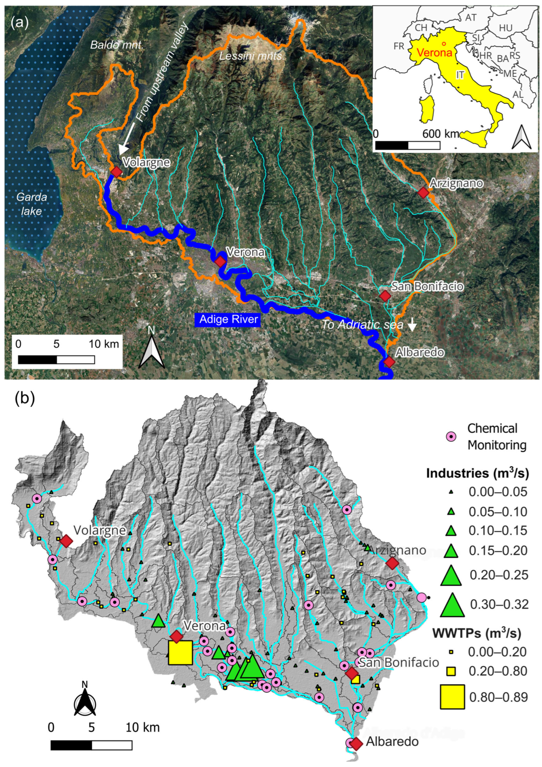
Figure 1. (a) Satellite image of the study area, including the main hydrological features (Adige River main branch, in blue, and its tributaries) and main municipalities. The orange line outlines the SWAT model extension. The Adige River enters the modeled area at Volargne and exits it at Albaredo. (b) Boundaries of the SWAT subbasins, in black, and discharge outlets from industries and wastewater treatment plants (WWTPs). The legend reports the average discharge rates in m3/s. Chemical monitoring points are also illustrated. The background hillshade map represents the digital elevation model (DEM).
Hydrology 12 00239 g001
Figure 2. Location of main diversions, weather stations and gauge stations used in this study.
Hydrology 12 00239 g002
Figure 3. Comparison between observed and simulated (a) streamflow rates (Q) and (b) total nitrogen (TN) concentrations at the Adige–Albaredo station. The 95% envelope is based on the measurement errors. (c) Mean annual TN loadings predicted by SWAT and calculated from measured concentrations at different monitoring points in the basin.
Hydrology 12 00239 g003
Figure 4. Average streamflow in the reference scenario (“default”) in the different water bodies of the modeled Adige basin. The figure does not show the final channeled part, as the outflow into the Adriatic is similar to that at Albaredo.
Hydrology 12 00239 g004
Figure 5. Top: difference in flow rates ( Δ Q ) between the reference model and the simulated climate change scenarios GWL = 2 °C (a) and GWL = 3 °C (b) temperature change. Bottom: cumulative Δ Q simulated in the three climate change scenarios for GWL = 2 °C (c) and GWL = 3 °C temperature change (d).
Hydrology 12 00239 g005
Figure 6. Distribution of total nitrogen (TN) loading (kilotons/year) in the main water bodies of the Adige basin.
Hydrology 12 00239 g006
Figure 7. Area-normalized total nitrogen (TN) mass (kg/ha) in the different subbasins for the calibrated scenario.
Hydrology 12 00239 g007
Figure 8. (a) Simulated time series of the monthly cumulated total nitrogen (TN) in the Adige River at Albaredo. (b,c) Difference in monthly loadings ( Δ L ) between the reference model and the simulated climate change scenarios, GWL = 2 °C and GWL = 3 °C temperature change, respectively. (d,e) Cumulative Δ L simulated in the three climate change scenarios.
Hydrology 12 00239 g008
Figure 9. Predicted difference in area-normalized total nitrogen (kg/ha) loadings calculated for the CNRM-2 °C scenario (a) and MPI-3 °C scenario (b), compared to the reference model.
Hydrology 12 00239 g009
Figure 10. Distribution of total phosphorus (TP) loadings (tons/year) in the main water bodies of the Adige basin.
Hydrology 12 00239 g010
Figure 11. (a) Simulated time series of the monthly cumulated total phosphorus (TP) in the Adige River at Albaredo. (b,c) Difference in monthly loadings ( Δ L ) between the reference model and the simulated climate change scenarios GWL = 2 °C and GWL = 3 °C temperature change, respectively. (d,e) Cumulative Δ L simulated in the three climate change scenarios for 2 °C and 3 °C temperature change, respectively.
Hydrology 12 00239 g011
Figure 12. (a) Area-normalized total phosphorus (TP) loadings (kg/ha) in the different subbasins for the reference scenario. (b,c) Predicted variation under the CNRM model at 2 °C and the MPI model at 3 °C compared to the reference scenario.
Hydrology 12 00239 g012
Figure 13. Year-cumulated total phosphorus (TP, in tons) simulated at the Adige–Albaredo control point.
Hydrology 12 00239 g013
Figure 14. Comparison between the reference model (dots) and models embedding elevated irrigation (blue line) and atmospheric deposition (dotted orange lines). The data refers to the cumulated total nitrogen (TN) loadings (TN/month) crossing the Adige–Albaredo monitoring station.
Hydrology 12 00239 g014
Table 1. Typical dosage (kg/ha) and management action dates, by crop type, in the Adige lowland basin. The percentage in the first column indicates the estimated amount of fertilizer effectively introduced to the soil. Differences between inorganic and organic fertilizers are indicated. The last two columns indicate the amount of elemental nitrogen (N) and phosphorus (P) used in the SWAT model. S: sowing; H: harvest; DFM: fresh dairy manure; n.a: not available.
Crop Type (Weight)
Sowing (S); Harvesting (H)
Fertilizer
Application Date
Fertilizer IDDosage
(kg/ha)
N (kg/ha)P (kg/ha)
Barley—inorganic (40%)
S:15-Nov; H:20-Jun
15-Oct06-24-243001831
20-Feb33-00-00130430
20-MarUrea150690
Barley—organic (60%)
S:15-Nov; H:20-Jun
10-OctDFMn.a.10518
10-Mar33-00-00130430
Wheat—inorganic (40%)
S:10-Apr; H:15-Nov
15-oct06-24-243001831
20-Feb33-00-00185610
20-AprUrea142650
Wheat—organic (60%)
S:10-Apr; H:15-Nov
10-OctDFMn.a.9116
20-Mar33-00-00250830
Appletree—inorganic (100%)
S:15-Mar; H:20-Sept
20-Mar21-0-0200420
2-Jul13-0-46150200
20-Oct12-6-18200245
Grassland—organic (100%)15-MarDFMn.a.30052
Maize—inorganic (28%)
S:10-Apr; H:15-Nov
20-Apr06-24-245003052
15-MayUrea2501150
10-JunUrea210970
Maize—organic (72%)
S:10-Apr; H:15-Nov
10-MarDFMn.a.15727
10-JunUrea2601190
Olive trees—inorganic (30%)
S:1-Mar; H:1-Nov
1-Mar20-10-10150306
2-MayUrea100460
Pastures—organic (100%)1-AprDFMn.a.17030
Potato—inorganic (34%)
S:27-Mar; H:1-Aug
15-Mar05-10-158354236
20-AprUrea150690
10-MayUrea140640
Potato—organic (66%)
S:27-Mar; H:1-Aug
15-MarDFMn.a.17931
20-Apr12-08-18100123
10-MayUrea140640
Rapeseed—inorganic (34%)
S:30-Sep; H:25-Jun
20-Feb15-15-154106227
20-Mar33-00-00250830
Rapeseed—organic (66%)
S:30-Sep; H:25-Jun
15-SepDFMn.a.9917
20-Feb15-15-15150232
20-Mar33-00-00200660
Soy—inorganic (100%)
S:30-Apr; H:5-Oct
20-Apr0-26-00200023
20-AprUrea65300
Sugar beet—inorganic (43%)
S:30-Apr; H:25-Jun
20-FebUrea130600
20-Feb18-46-001502730
15-Apr33-00-00200660
Sugar beet—organic (57%)
S:30-Apr; H:25-Jun
20-FebDFMn.a.8615
15-AprUrea2301060
Sunflowers—inorganic (35%)
S: 10-Apr; H: 30-Aug
1-Apr0-15-0150010
1-Apr28-10-10150426
20-MayUrea150690
Sunflowers—organic (65%)
S: 10-Apr; H: 30-Aug
1-AprDFM08415
20-MayUrea145670
Grape—inorganic (89%)
S:15-Mar; H:1-Sep
30-Mar21-00-00150320
2-Jun27-0-0100270
20-Oct06-08-154002414
Grape—organic (89%)
S:15-Mar; H:1-Sep
30-Mar21-00-00150320
2-Jun27-0-0100270
20-OctDFM0305
Table 2. List of SWAT-CUP parameters modified during the model calibration using the SUFI-2 algorithm. The change could be performed by relative variation (“r”) of the parameter or by replacing (“v”) the reference parameter using a random value sampled from the parameter space bounded by the “min” and “max” values.
Parameter NameDescriptionUnitsMinMaxCalibrated
r__CN2.mgtMoisture condition II curve number-−0.500.50−0.30
v__ALPHA_BF.gwBaseflow recession constant-0.001.000.71
v__GW_DELAY.gwDelay time for groundwater recharged30.00450.00433.62
v__GWQMN.gwThreshold depth of water in the shallow aquifer required for return flow to occurmm H2O0.002.000.92
v__GW_REVAP.gwGroundwater revap coefficient-0.000.200.14
v__ESCO.hruSoil evaporation compensation factor-0.801.000.82
v__CH_N2.rteManning’s coefficient tributary channels-0.000.300.14
v__CH_K2.rteHydraulic conductivity of riverbedmm hr−15.00130.0010.88
v__ALPHA_BNK.rteBank flow recession constant-0.001.000.78
r__SOL_AWC(1).solSoil available water capacity-−0.200.400.38
r__SOL_K(1).solSaturated hydraulic conductivitymm hr−1−0.800.80−0.49
r__SOL_BD(1).solMoist bulk densityg cm−3−0.500.60−0.48
v__SFTMP.bsnSnowfall temperature°C−10.0010.00−5.10
r__OV_N.hruManning’s coefficient[-]−0.200.200.17
r__HRU_SLP.hruSlope lengthm0.000.500.05
r__SLSUBBSN.hruAverage slope lengthm0.000.500.28
Table 3. Combinations of climate models whose data were used as input for the climate change analyses carried out in this study. GCM = global circulation model. RCM = Regional climate model. GWL = Global warming level.
GCMRCMGWL 2 °CGWL 3 °C
Corresponding period
CNRM-CM5ICTP RegCM4-62035–20522057–2076
ICHEC-EARTHICTP RegCM4-62024–20432050–2069
MPI-ESM-LRICTP RegCM4-62027–20462051–2070
Table 4. Summary statistics from the model calibration. Details regarding specific meaning of each statistic can be found in [54].
Summary StatisticsShort DescriptionAlbaredoVerona
NSENash Sutcliffe error [-]0.760.69
p-factorPercentage of values within the 95% interval [-]0.630.28
r-factor95% envelop thickness [-]0.540.10
R2Coefficient of determination [-]0.850.89
bR2Modified R2 [-]0.840.70
MSEMean square error [m6/s2]2400.001900.00
SSQRRanked square errors [m6/s2]860.001200.00
PBIASPercent bias [-]12.00−11.80
KGEKling-Gupta efficiency [-]0.840.63
RSRStandardized RMSE [m3/s]0.490.56
MNSModified Nash Sutcliffe coefficient [-]0.500.46
VOL_FRfraction of the overall water balance that is predicted [-]1.140.89
Mean sim (Mean obs)Average simulated (observed) values [m3/s]192.16 (218.31)156.65 (140.11)
Std Dev sim (Std Dev obs)Standard deviation of the simulated (observed) values [m3/s]106.79 (99.92)104.01 (77.30)
Table 5. Summary of the average monthly cumulative precipitation values (mm) for the Adige basin for the observed (“reference”) data and the downscaling of climate models. The table also reports the “control” values of each model (2001–2020).
ModelScenarioJanFebMarAprMayJunJulAugSepOctNovDec
CNRMControl57.573.775.893.5118.886.183.795.896.8104.5136.181.6
GWL = 2 C71.284.858.3116.3115.377.689.5116.593.5115.5208.471.1
GWL = 3 C92.879.272.3112.0119.194.491.1105.0115.2103.2167.594.2
ICHECControl57.573.775.893.5118.886.183.795.896.8104.5136.181.6
GWL = 2 C86.0117.7111.473.086.583.274.9114.783.689.7100.685.5
GWL = 3 C108.3102.8108.1106.396.890.1127.582.194.589.397.9122.1
MPIControl57.573.775.893.5118.886.183.795.896.8104.5136.181.6
GWL = 2 C41.566.584.195.6139.5106.574.2108.298.9123.3109.868.8
GWL = 3 C59.086.183.6114.0142.6104.364.673.6115.0167.6167.357.6
Reference58.274.176.193.9119.286.684.296.397.2105.3136.782.5
Disclaimer/Publisher’s Note: The statements, opinions and data contained in all publications are solely those of the individual author(s) and contributor(s) and not of MDPI and/or the editor(s). MDPI and/or the editor(s) disclaim responsibility for any injury to people or property resulting from any ideas, methods, instructions or products referred to in the content.