Generalized Methodology for Two-Dimensional Flood Depth Prediction Using ML-Based Models

Abstract

Floods are among the most devastating natural disasters; predicting their depth and extent remains a global challenge. Machine Learning (ML) models have demonstrated improved accuracy over traditional probabilistic flood mapping approaches. While previous studies have developed ML-based models for specific local regions, this study aims to establish a methodology for estimating flood depth on a global scale using ML algorithms and freely available datasets—a challenging yet critical task. To support model generalization, 45 catchments from diverse geographic regions were selected based on elevation, land use, land cover, and soil type variations. The datasets were meticulously preprocessed, ensuring normality, eliminating outliers, and scaling. These preprocessed data were then split into subgroups: 75% for training and 25% for testing, with six additional unseen catchments from the USA reserved for validation. A sensitivity analysis was performed across several ML models (ANN, CNN, RNN, LSTM, Random Forest, XGBoost), leading to the selection of the Random Forest (RF) algorithm for both flood inundation classification and flood depth regression models. Three regression models were assessed for flood depth prediction. The pixel-based regression model achieved an R² of 91% for training and 69% for testing. Introducing a pixel clustering regression model improved the testing R² to 75%, with an overall validation (for unseen catchments) R² of 64%. The catchment-based clustering regression model yielded the most robust performance, with an R² of 83% for testing and 82% for validation. The developed ML model demonstrates breakthrough computational efficiency, generating complete flood depth predictions in just 6 min—a 225× speed improvement (90–95% time reduction) over conventional HEC-RAS 6.3 simulations. This rapid processing enables the practical implementation of flood early warning systems. Despite the dramatic speed gains, the solution maintains high predictive accuracy, evidenced by statistically robust 95% confidence intervals and strong spatial agreement with HEC-RAS benchmark maps. These findings highlight the critical role of the spatial variability of dependencies in enhancing model accuracy, representing a meaningful approach forward in scalable modeling frameworks with potential for global generalization of flood depth.

1. Introduction

Floods are among the most widespread and destructive natural hazards, frequently resulting in severe loss of life and significant economic damage. With the increasing volatility of weather patterns driven by climate change, the frequency and severity of flood events are projected to rise [1]. This growing threat underscores the urgent need for preventive and responsive strategies to mitigate the impact of flooding on communities and infrastructure. Preventive measures aim to assess and communicate the likelihood of flooding in specific areas, often through the use of flood depth maps—tools that illustrate potential inundation levels under various conditions [2]. In contrast, emergency measures are implemented immediately before, during, or following a flood event, and require near-real-time information on flood extent and affected areas to enable timely and effective decision-making [3].

Flood Early Warning Systems (FEWSs) play a crucial role in minimizing flood impacts through timely alerts and preparedness. However, their effectiveness is often hindered by high computational demands and challenges in accessing and integrating real-time hydroclimatic data—especially in developing regions. Traditional FEWSs depend on complex hydrological and hydrodynamic models that require intensive calibration, data assimilation, and expert knowledge, limiting their scalability and operational efficiency [4]. These processes are time-consuming and computationally intensive, particularly when ensemble simulations or real-time scenario forecasting are needed. In many regions, the lack of high-quality input data, such as LiDAR-based topography or accurate rainfall estimates, further reduces model reliability. Improving model efficiency, enhancing computational infrastructure, and automating data assimilation workflows are critical steps toward increasing the predictive accuracy and practical feasibility of FEWSs [4,5]. To overcome these limitations, developers and practitioners have recommended the application of ML algorithms in flood modeling and analysis [6].

Machine learning (ML) is a subset of artificial intelligence where algorithms enhance their performance by learning from increasing amounts of data and repeated task execution [7]. The model’s performance can then be enhanced by uncovering hidden patterns in the data. In hydraulics and flood studies, ML models have been used geographically and temporally [8]. While most flood research has focused on temporal modeling (such as rainfall runoff), spatial flood mapping remains underdeveloped. Understanding flood spatial dynamics is essential for predicting inundation and informing emergency response.

Due to the high computational cost of traditional models, machine learning (ML) is gaining traction as a faster alternative. However, there is still a significant gap in developing robust, scalable ML models explicitly tailored for spatial flood prediction. Addressing this gap is vital for advancing practical flood risk management solutions [9]. Accurate prediction of maximum flood depth in ungauged catchments remains a critical challenge, limiting the effectiveness of current flood risk management strategies. Flood depth maps provide estimates of inundation depth and spatial coverage for different rainfall scenarios and return periods. These maps are typically generated using numerical hydrodynamic models, which simulate flood behavior by discretizing the governing equations and the spatial domain. In addition to depth, such models can also simulate flow velocities, offering a more comprehensive representation of flood dynamics.

Over the past three decades, numerous numerical hydrodynamic modeling tools such as HEC-RAS and MIKE 21 have been developed for this purpose [10,11]. With the widespread availability of high-resolution spatial data, particularly in low-relief terrain, two-dimensional (2D) hydraulic models have become increasingly utilized. These models discretize the computational domain into a mesh of cells, allowing for detailed simulation of flood dynamics across complex topographies. Due to their ability to simulate the lateral components of the shallow water equations, 2D models are well-suited for floodplain mapping and flood depth estimation [12,13,14,15].

Although current 2D numerical methods are considered reliable and effective for flood analysis, both expert and non-expert modelers often encounter challenges in achieving rapid and accurate simulations [12]. The computational intensity of these models results in longer processing times, posing a significant barrier to their use in time-sensitive applications [12]. Various efforts have been made to accelerate simulation times, such as the adoption of parallel computing techniques [12,16,17]. However, these approaches typically require access to high-performance computing resources, which may not be widely available or cost-effective [12]. These computational constraints present a critical limitation in developing near-real-time flood forecasting and response tools. This affects the reliability and timeliness of flood early warning systems, which are crucial for reducing flood impacts, improving emergency preparedness, and enhancing community resilience. For instance, the small stream flood early warning system SSFEWs developed by Cheong et al. 2024 [5] demonstrated root mean squared errors (RMSEs) of up to 0.619 m³/s for discharge and 0.016 m for water depth. However, the system’s accuracy declined when rainfall forecasts extended beyond one hour, highlighting the sensitivity of such models to input uncertainty and the limitations of near-real-time flood forecasting applicability [5]. In this context, ML-based approaches offer a practical pathway to overcoming these challenges, enhancing the responsiveness and adaptability of FEWSs by reducing computational overhead and enabling more timely predictions [5].

Machine learning (ML) surrogate models, such as U-FLOOD, have emerged as promising alternatives to traditional numerical approaches, offering faster and more computationally efficient solutions without significantly compromising predictive accuracy. These models are particularly advantageous in operational settings where rapid forecasting is essential [9].

Costache et al. (2024) proposed an ensemble modeling approach combining deep learning, Harris Hawk Optimization, and stacking-based machine learning for flood mapping in Romania’s Buzău River basin [18]. This study used 12 predictors and 410 data points, achieving high accuracy, particularly with the developed model. While effective locally, this study highlights the challenges of generalizing these models to different regions, emphasizing the need for further research to enhance global applicability [18].

Dai et al. (2024) developed an ensemble Artificial Neural Network (EANN) model to enhance urban flood prediction in coastal areas such as Macao, China [19]. The model effectively predicted flood depths during typhoon events, demonstrating that short training datasets can yield high accuracy. However, this study highlights the challenges posed by uncertainties in input data and model parameters, which remain critical for accurate flood forecasting [19].

Seleem et al. (2023) used Convolutional Neural Networks (CNNs) and Random Forest (RF) models to predict urban pluvial floodwater depth in Berlin [20]. RF performed well within the training domain using inputs such as rainfall, topography, and land use, but showed poor transferability due to overfitting. In contrast, CNNs—especially U-Net-based architectures—demonstrated better adaptability to new areas via transfer learning. However, this study’s reliance on a geographically limited dataset constrained its broader applicability to urban regions with different hydrological conditions [20].

Esmaeili-Gisavandani et al. (2023) utilized three data-driven models—RF, Adaptive Network-based Fuzzy Inference System (ANFIS) [21,22], and a decision tree algorithm to perform regional flood frequency analysis (RFFA) in ungauged catchments in the Karkheh River basin, Iran. Compared with traditional multivariate regression, the RF model yielded the most accurate predictions of peak flows across various return periods. This study demonstrated RF’s effectiveness in handling hydrological data uncertainty but also noted limitations in transferring the model to catchments with different hydrological characteristics [22].

Balestra et al. (2022) applied deep neural networks in Southern Italy and demonstrated that such models can rapidly delineate flood-prone areas by relying on globally reproducible conditioning factors [23]. This approach is particularly valuable in regions where traditional hazard maps are unavailable [23]. In parallel, Chen et al. (2019) proposed a hybrid ensemble framework that integrated reduced-error pruning trees with bagging and random subspace ensembles, achieving superior predictive performance and highlighting the effectiveness of ensemble techniques for flood susceptibility modeling [24]. Collectively, these studies emphasize both the scalability of neural networks and the robustness of ensemble-based approaches, underscoring the importance of integrating diverse ML strategies into flood risk assessment.

Overall, using machine learning (ML) in flood prediction can significantly improve flood management and mitigation efforts worldwide, helping to save lives and reduce damage from flooding events [9]. However, efforts to develop a general or global model remain limited because of the problem’s complexity and the constraints of available data, which restrict the machine learning model’s ability to perform well in unseen regions [9,25].

Combining unsupervised and supervised machine learning techniques has been shown to improve the generalization and transferability of models. Unsupervised techniques, such as clustering and dimensionality reduction, can help identify patterns and relationships in the data that may not be apparent through manual inspection. Supervised techniques, such as classification and regression, can then be used to build models that predict outcomes based on the identified patterns, allowing them to perform better on new and unseen data [24,26,27,28].

While HEC-RAS 2D remains a widely used tool for flood inundation modeling, its simulations are computationally intensive and time-consuming. This study aims to develop a data-driven surrogate modeling approach that delivers comparable flood depth predictions in a fraction of the time, achieving notable improvement in computational efficiency. The approach is particularly valuable for vulnerable ungauged catchments, where timely flood prediction is crucial for risk mitigation. Despite the growing use of machine learning in hydrology, existing studies often rely heavily on observed data, which are sparse in many regions, and few integrate clustering and model generalization to scale flood predictions spatially.

This research addresses these gaps by introducing a novel, cluster-integrated machine learning framework trained on hydrodynamically simulated data. It combines geospatial feature extraction, unsupervised clustering, and regression modeling to enable accurate, near-real-time, pixel-level flood depth prediction. The novelty lies not only in methodological integration but also in its operational value supporting early warning systems and enabling faster, more informed decision-making in flood-prone areas.

2. Materials and Methods

To ensure both reliability and scalability, strict data selection criteria were applied in accordance with IPCC recommendations [29]. In particular, only datasets that were (i) the most recent and updated, (ii) of the highest available resolution, and (iii) globally consistent were used. Adhering to these criteria enhances the accuracy of the modeling framework while supporting its applicability for broader generalization. Furthermore, the model architecture was designed to remain flexible, allowing seamless integration of future datasets as they become available and refined [29].

2.1. Freely Available Datasets

This study uses the ALOS World 3D (AW3D30) dataset from the Advanced Land Observing Satellite (ALOS) to obtain high-precision global elevation data https://www.eorc.jaxa.jp/ALOS/en/aw3d30/index.htm (accessed on 10 March 2023) [30].

In addition, this study used the Environmental Systems Research Institute (ESRI) worldwide cover LULC map (LULC 2020-ESRI) [31], which was developed from Sentinel-2 [32]. The Global Hydrologic Soil Groups (HYSOGs 250m) dataset, developed by Ross et al. (2018) [33], provides a globally consistent, gridded classification of hydrologic soil groups (HSGs) at a spatial resolution of approximately 250 (m) [33]. This dataset supports the United States Department of Agriculture (USDA) based curve number (CN) runoff modeling, which is essential for regional and continental-scale hydrological analyses [33]. This dataset was used along with the LULC dataset to identify the CN values for the modeling process. The Manning’s roughness (n) values based on land use/land cover datasets are essential for accurately modeling hydrological processes and predicting flood events [34]. This study incorporates weighted average Manning’s roughness coefficient (“n”) values derived by Soliman et al. (2022) [31].These values were calculated by comparing land cover classifications between the global ESRI LULC 2020 maps and the NLCD 2019 dataset, providing critical surface friction parameters for hydrological modeling [31].

2.2. Research Methodology

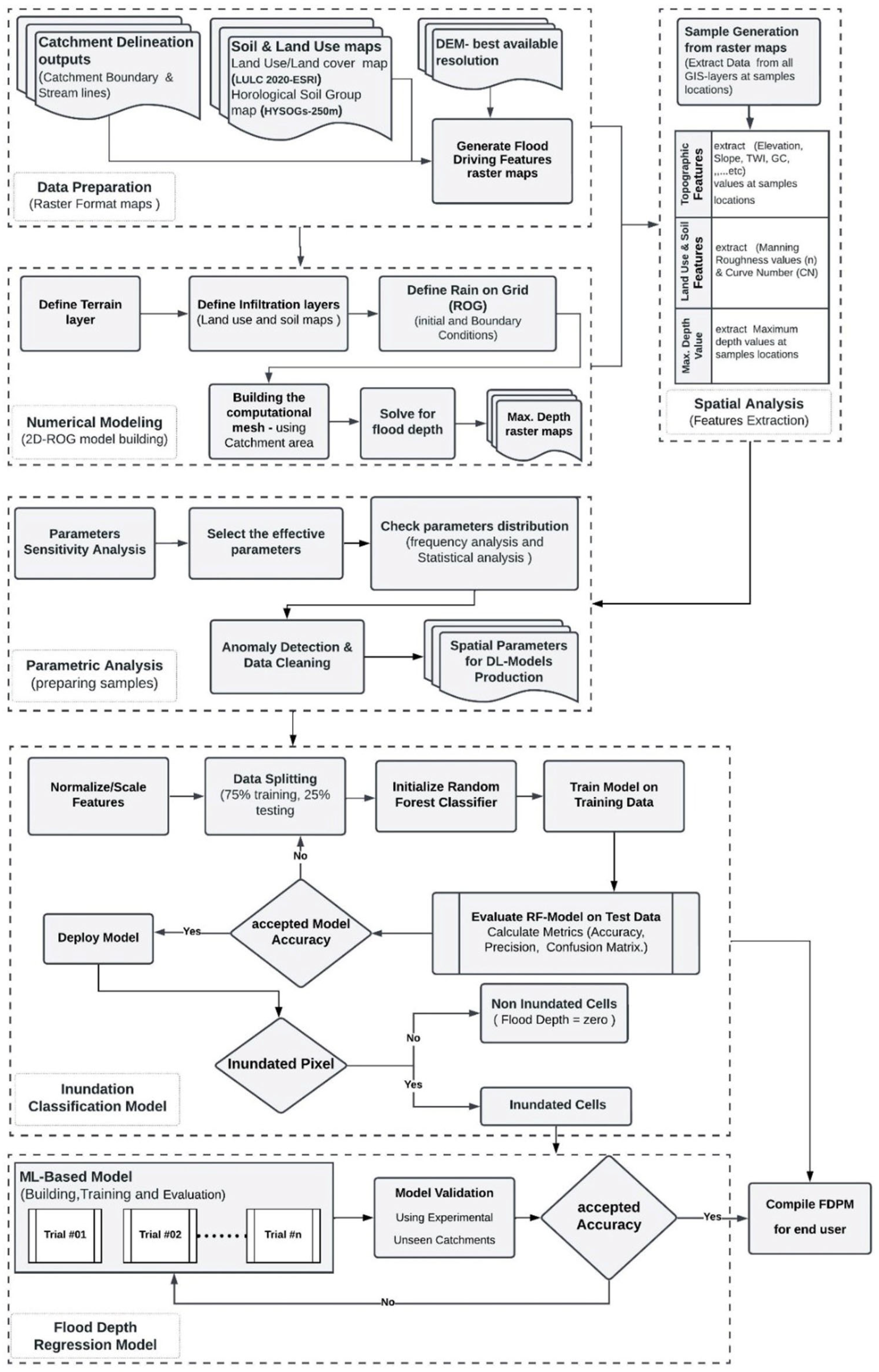
Figure 1 shows the general approach and methodology applied to conduct the research, which includes six stages.

2.2.1. Stage 1: Data Preparation

The first step in developing a generalized flood depth prediction model involves comprehensive data preparation. This step involved three key tasks:

• Dataset collection: High-resolution DEMs were used to extract elevation, slope, and aspect, and to delineate catchments and stream networks. Land use/land cover data were obtained from the ESRI 2020 dataset, while soil properties were taken from the HYSOGs-250m database [31].
• Hydrological parameter derivation: These datasets were integrated to generate an SCS-CN infiltration raster map. Manning’s roughness coefficient (n) and the Curve Number (CN) were derived from the land cover and soil data [31,35].
• Integration for modeling: The resulting topographic, infiltration, and roughness parameters provided the essential inputs for subsequent 2D hydrodynamic simulation and machine learning analysis.

2.2.2. Stage 2: 2D Numerical Hydrodynamic Modeling

Flood events were simulated using 2D hydrodynamic Rain-on-Grid (RoG) models in HEC-RAS Version 6.3. This process involved three key steps:

• Model construction: Terrain data, land use/land cover, precipitation inputs, and SCS-CN infiltration rasters were combined to construct the 2D ROG model [36,37,38,39,40,41,42].
• Flood simulations: Unsteady flow was solved under coupled 1D–2D conditions. The 2D domain was discretized into computational cells, with flow factors calculated between neighboring cells to estimate water movement and depth [34].
• Output generation: Raster maps of maximum flood depth were produced for each catchment, representing inundation patterns and forming the training data for ML modeling [31,36,37].

2.2.3. Stage 3: Spatial Analysis

Spatial analysis was conducted to extract relevant features from the prepared datasets. Data samples were generated by extracting values from all raster maps at predefined locations, compiling a feature set that captured topographic, hydrologic, and land-surface characteristics for model training.

2.2.4. Stage 4: Parametric Analysis (Preparing Samples)

For a rigorous parametric analysis, a framework was implemented to refine the dataset and improve model reliability.

• Parameter sensitivity evaluation—Distribution analysis and Random Forest-based sensitivity testing [20] were used to quantify the relative importance of input parameters for flood depth predictions [23].
• Statistical validation—Data normality was examined using the Kolmogorov-Smirnov (K-S) test, alongside descriptive statistics (skewness and kurtosis) [43,44].
• Outlier detection and refinement—Z-scores were applied to normally distributed variables, while the interquartile range (IQR) method was used for non-normal distributions. This step ensured data quality, supporting better generalization and predictive accuracy [20,45,46].

2.2.5. Stage 5: Inundation Classification Model

The classification pipeline was designed to distinguish between inundated and non-inundated areas.

• Features were normalized and scaled to ensure consistency across algorithms.
• The dataset was split into training (75%) and testing (25%) subsets, with balanced sampling applied to improve classification accuracy.
• A Random Forest Classifier (RFC) was trained and evaluated using performance metrics including confusion matrix, accuracy, and precision [47,48].

2.2.6. Stage 6: Flood Depth Regression Model

The final stage focused on pixel-level prediction of maximum flood depth using machine learning regression models. Six representative algorithms were selected to capture diverse learning strategies:

• Tree-based ensembles—Random Forest (RF) and XGBoost (XGB) were applied for their robustness, interpretability, and ability to model non-linear relationships.
• Neural networks—Artificial Neural Network (ANN), Convolutional Neural Network (CNN), Recurrent Neural Network (RNN), and Long Short-Term Memory (LSTM) models were used for their ability to capture complex, high-dimensional, and sequential patterns in geospatial and hydrological datasets [9].

Model performance was assessed using statistical evaluation metrics and validated against observed or calibrated flood depth data from experimental catchments. The comparative results provided a comprehensive assessment of different ML strategies and their potential for generalized flood depth prediction.

3. Results

3.1. Stage 1: Data Preparation

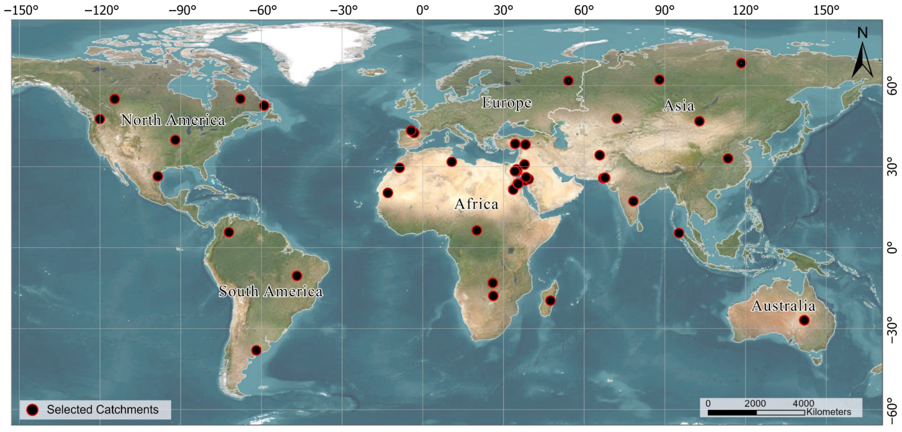
To prepare training data, 45 catchment areas were selected randomly based on maximizing the variability of flood-driving parameters (see Figure 2 for catchment locations). The selected catchments were delineated and then analyzed based on elevation, land use/land cover, and soil type to verify global coverage and variability.

The selected catchment area outlet locations, average elevations, and dominant infiltration parameters are presented in

Table A1. Selected catchments study areas, outlet locations, average elevations, and dominant infiltration parameters.

Catchment ID	Region	Country	Outlet Location (UTM-WGS 84)		Catchment Area (km2)	Average Elevation (m)	Dominant Land Use and Land Cover	Dominant Soil Type *
			Latitude (°)	Longitude (°)
CA-01	Africa	Libya	31.75800	10.75300	321.56	570.70	Shrub/Scrub	B
CA-02	Asia	India	17.16700	78.32300	154.33	629.05	Crops/Built Area	C/D
CA-03	Asia	Pakistan	25.67800	67.10900	109.78	480.98	Shrub/Scrub	C
CA-04	Asia	Pakistan	25.85000	67.72700	234.56	392.63	Shrub/Scrub	C/B
CA-05	Asia	Mongolia	46.80400	102.83700	500.85	1916.84	Grass	C
CA-06	Asia	Kazakhstan	47.80700	72.16200	703.68	804.81	Shrub/Scrub	C
CA-07	Europe	Russia	68.35800	118.40500	571.82	294.54	Trees	C
CA-08	Europe/Asia	Turkey	38.19800	38.19800	94.72	1817.09	Shrub/Scrub	C
CA-09	Europe/Asia	Turkey	38.42200	34.38800	173.37	1296.59	Crops	C
CA-10	Africa	Mauritania	20.28700	−13.00000	213.22	573.10	Shrub/Scrub	C
CA-11	Africa	Morocco	29.57300	−8.62400	34.47	1493.22	Bare Ground	B/C
CA-12	Africa	Zambia	−13.10400	26.05900	40.71	1361.20	Trees	D
CA-13	Africa	Madagascar	−19.65000	47.49100	3.75	1616.52	Shrub/Scrub	D
CA-14	North America	United States	26.39500	−98.47100	289.98	117.09	Shrub/Scrub/ Crops	C
CA-15	South America	Colombia	5.70900	−72.04300	78.83	453.13	Trees/ Shrub/Scrub	C/D
CA-16	Asia	China	33.03800	113.49000	63.41	284.18	Crops	C
CA-17	Asia	Afghanistan	34.23100	65.80500	259.62	2998.15	Shrub/Scrub	C
CA-18	South America	Brazil	−10.48600	−46.77200	101.83	484.23	Shrub/Scrub	C/D
CA-19	North America	Canada	55.11700	−67.78200	207.46	572.64	Trees/water	D
CA-20	Europe/Asia	Russia	61.78800	54.14400	234.54	214.01	Trees	C/D
CA-21	Europe/Asia	Russia	62.22200	88.01400	321.93	215.84	Trees	C/D
CA-22	Africa	Central African R.	6.32600	20.10300	719.88	558.59	Trees	D
CA-23	North America	Canada	55.03800	−114.56600	147.44	761.50	Trees	D/D
CA-24	North America	Canada	52.57800	−58.99100	76.78	515.03	Trees/snow/Ice	D-D/D
CA-25	South America	Argentina	−38.07100	−61.83100	344.19	462.89	Shrub/Scrub/Grass	C
CA-26	Asia	Jordan-KSA	30.76519	37.83196	74.70	584.92	Shrub/Scrub	C
CA-27	Asia	KSA	24.91416	37.99900	64.20	1007.03	Shrub/Scrub	C
CA-28	Asia	KSA	25.37081	39.35818	87.20	910.59	Bare Ground/Shrub/Scrub	C
CA-29	Africa	Sudan	21.49940	33.62773	531.00	473.76	Shrub/Scrub	B/C
CA-30	Africa	Egypt	23.66718	35.27256	242.00	515.04	Bare Ground/Shrub/Scrub	C
CA-31	Africa	Egypt	23.68637	35.33446	58.30	514.51	Bare Ground/Shrub/Scrub	C/D
CA-32	Africa	Egypt	23.62521	35.43380	40.90	311.46	Bare Ground/Shrub/Scrub	B
CA-33	Asia	KSA	26.05159	38.46643	28.40	886.60	Shrub/Scrub	B/C
CA-34	Asia	KSA	28.43663	35.10055	48.70	697.08	Bare Ground	C
CA-35	Asia	KSA	28.63930	34.79806	20.80	645.90	Bare Ground	C
CA-36	Asia	KSA	28.99278	34.90504	11.40	672.97	Bare Ground	C
CA-37	Africa	Egypt	28.29316	34.30254	246.00	997.06	Crops/Bare Ground	C
CA-38	Europe	Spain	42.50198	−3.17814	10.00	779.31	Crops	C
CA-39	Europe	Spain	43.38476	−4.32133	25.70	83.75	Trees/Grass/Built Areas	C
CA-40	Australia	Australia	−26.88829	141.81263	183.00	132.30	Shrub/Scrub	C/D
CA-41	Australia	Australia	−26.97191	141.87039	75.90	115.00	Shrub/Scrub	C/D
CA-42	Asia	Malaysia	5.37901	95.25945	110.00	712.39	Trees	C
CA-43	Africa	Zambia	−17.91887	26.24845	117.00	1137.03	Crops	D
CA-44	North America	United States	39.87476	−92.02406	149.17	245.60	Trees/Crops	C/D
CA-45	North America	United States	47.64708	−120.05396	7.85	836.52	Built Areas /Crops	C

* Hydrological Soil Groups (HSGs) classify soils into four groups (A–D) based on their infiltration rate and runoff potential. Group A has high infiltration and low runoff, while Group D has very low infiltration and high runoff, with B and C being intermediate [33].

.

3.2. Stage 2: 2D Numerical Hydrodynamic Modeling

Numerical hydrodynamic modeling was conducted using the HEC-RAS Version 6.3 2D ROG simulation across 45 selected catchments, with precipitation values ranging from 20 to 500 mm in incremental intervals for 24 h. The depth raster maps generated from these simulations were systematically saved for further extraction and analysis to assess the sensitivity of various parameters and explore the trends and physical relationships among them. The total number of samples was 9.04 million pixels (each 30 m × 30 m, the same resolution as the DEM) with a total catchment area of 8135 km², ranging from 3.75 km² to 719.88 km². However, for building the classification and regression models later in the research, a fixed rainfall event with a moderate value of 100 mm was selected to ensure consistent and controlled analysis [40]. The forty-five global and six validation catchment simulations used adaptive time stepping with a 1 s base time step and 30 (m) cell size. A conservative Courant number limit of 1.0 was applied to ensure model stability. This setup enabled accurate resolution of flow dynamics across varying topographic and hydrologic conditions. Uniform configurations supported consistent performance evaluation across all catchments [34,40].

3.3. Stage 3: Spatial Analysis and Flood-Driving Parameters

Based on the literature review, it was found that the number of flood susceptibility parameters implemented in each study varies between 5 and 21 parameters [9]. To select the most repeated and effective parameters, an extensive review of 25 research studies [9,20,49] was conducted, and 12 effective parameters were selected based on the number of repetitions of each parameter for the reviewed research as an initial step to be verified during this study. The main driving parameters can be categorized as follows:

• Topographical parameters derived from a digital elevation model, such as elevation, slope, and aspect.
• Meteorological parameters related to hydrological characteristics, such as rainfall depth.
• Infiltration driving parameters such as land use/land cover and soil dataset.

Table 1. Flood predictive parameters and their description, range in the study, and number of repetitions in the reviewed papers [9,20,49].

Parameter Category	Predictive Parameter	Description	Range in This Study	Repetitions in Reviewed Research
Topographical	Elevation	Land surface elevations derived from globally used DEMs [49,50].	[0–3752] (m)	23
	Slope	Terrain slope impacts the runoff velocity and the available time for infiltration [51].	[0–1.571]	24
	Aspect	Aspect characterizes flow direction on terrain [20,50].	[0–6.283]	16
	Topographic Wetness Index (TWI)	Topographic wetness index is defined as ln (α/tan(β)) with α being the contributing area per unit contour length and β the local terrain slope. Measures the tendency of an area to accumulate runoff [47,50].	[−4.5–15.1]	18
	Curvature	Curvature characterizes concaveness/convexity of terrain pixel [20,50].	[−0.75–1.00]	17
	Sink (SD)	Sink depth, depth of terrain sinks. Computed as the difference between the elevation of the outlet point of a sink and the terrain elevation [20,50].	[0.761–52.96]	2
	Flow Accumulation (FAC)	Flow accumulation value, the number of cells flowing into a given pixel. Describes the likelihood of depression being flooded [20,50].	[0–486,709]	8
	Distance to Stream (DTS)	Distance to stream measures the distance between the point/cell and the nearest stream [20].	[0–9841]	15
	Topographic position index (TPI)	Topographic position index is defined as the difference between the pixel elevation and the mean elevation of the surrounding pixels. A positive value denotes that the pixel is higher than the neighboring pixels, while a negative value indicates that the pixel is lower than the neighboring pixels, and a zero value represents flat areas [20].	[−45.25–100]	2
Land Use\Land Cover\Soil	Curve number (CN)	Curve number is an empirical parameter that is computed using land cover and soil hydrologic group. It is used to estimate the direct runoff. We used the CN values produced by TR-55 [35].	[32–98]	4
	Roughness (n)	Roughness impacts the excess runoff flow over the surface. We used the global LULC maps along with Manning roughness coefficient values produced by [31].	[0.025–0.35] (s·m−1/3)	2
Meteorological	Precipitation Depth (PD)	Precipitation depth, we used 24 h duration precipitation events with precipitation depth [20].	[20,50,100,150,200,300,500]	20

shows the selected 12 predictive features considered potentially relevant for mapping flood depths and their description. The topographic predictive features were generated from a DEM described in the materials section.

While the machine learning models could not “understand” the physical processes of rainfall runoff generation, they are designed to detect relationships between input and target variables [52], in this case, simulated inundation depth. Therefore, predictive features should represent the surface characteristics of the study area (topography and land use/land cover) in addition to the precipitation depth. This could inform the model of governing hydrological and hydrodynamic patterns and relations.

3.4. Stage 4: Parametric Analysis

3.4.1. Parameter Sensitivity Analysis

Sensitivity analysis is a fundamental approach in scientific research for assessing the impact of input parameters on a model’s output. It aims to understand how variations in input values influence the model’s predictions or outcomes. In the context of machine learning, RF provides a powerful tool for conducting sensitivity analysis of input parameters. To perform a sensitivity analysis using RF, the input parameters are considered features, and the corresponding output variable (inundation depth) is the target for prediction. The impact of each parameter on the model’s predictions can be quantified by training the RF model on a dataset with varying input parameter values. The feature importance scores generated by RF measure the relative influence of input parameters on the output variable. The sensitivity of the flood-driving parameters on the depth prediction in the current study is illustrated in Figure 3.

The DTS shows the most sensitive parameter with 24% importance. Then SINK comes afterward with a percentage of 14.5% importance. CN and Manning’s n were identified as the least sensitive parameters, with important scores of 2.3% and 1.7%, respectively, indicating that land use-related factors have only a minor influence on the model’s performance compared with other geospatial parameters.

3.4.2. Flood-Driving Parameters Statistical Analysis

The selected catchments are imported to the GIS application to calculate the parameters from raster images and then extract the samples (points/pixels) at specific locations on a 30 m grid. The extracted parameters at each pixel location and their descriptive statistics are summarized in

Table A2. Descriptive statistics used to extract parameters in the study areas.

Parameter	ELV	ASPECT	SLOPE	DTS	GC	TWI	CN	n	FAC	TPI	SINK
unit	(m)	radians	radians	(m)	(unitless)	(unitless)	(unitless)	(s·m−1/3)	number of cells	(unitless)	(m)
Mean	855.083	3.094	0.190	1755.693	0.5402	8.720	79.543	0.055	383.595	11.087	0.108
std.	724.538	1.804	0.315	1738.237	0.1934	2.567	5.016	0.045	6680.393	192.202	0.678
Min.	−3.572	0.000	0.000	0.000	−0.750	−4.496	32.000	0.025	0.000	−45.250	0.000
Q1	453.853	1.554	0.028	418.760	−0.001	8.157	77.000	0.027	0.000	−0.875	0.000
Q2	591.873	3.066	0.065	1053.744	0.000	9.067	79.000	0.027	1.000	0.000	0.000
Q3	949.833	4.657	0.230	2742.557	0.001	9.860	85.000	0.092	6.000	0.850	0.000
Max.	3752.000	6.283	1.571	9841.025	1.000	15.056	98.000	0.350	486,709.0	100.000	38.366
Median	591.873	3.066	0.065	1053.744	0.000	9.067	79.000	0.027	1.000	0.000	0.000
Skewness	1.629	0.049	3.284	1.234	0.274	−2.974	0.100	1.836	38.505	17.330	11.937
Kurtosis	2.095	−1.183	11.382	0.822	280.323	11.272	0.991	5.330	1977.004	299.327	220.645
CV	0.847	0.583	1.661	0.990	3579.906	0.294	0.063	0.827	17.415	17.336	6.258

(Appendix A).

3.4.3. Check Data Probability Distribution

The analysis excludes the parameters CN, n, and rainfall as they are discrete values that do not follow any probability density function (PDF). The statistical analysis of the dataset parameters revealed significant deviations from normal distribution through two complementary methods. The Kolmogorov–Smirnov (K-S) test demonstrated statistically significant results for all parameters, with the calculated D-values substantially exceeding the critical threshold of 0.00045 (α = 0.05, n = 9.04 million), firmly rejecting the normality assumption (See Appendix A,

Table A3. Normality check (K-S) test result.

Predictive Parameter	Statistics (D)	Predictive Parameter	Statistics (D)
ELEV	0.2144	Twi	0.1892
Aspect	0.0596	FAV	0.4771
Slope	0.2736	TPI	0.4946
DTS	0.1622	sink	0.4899
GC	0.4827

). This conclusion was further supported by descriptive statistics analysis, where the observed skewness and kurtosis values for all parameters markedly differed from the expected normal distribution benchmarks; see Table A2. The consistent findings from both analytical approaches—the parametric K-S test and non-parametric descriptive statistics—provide robust evidence of non-normal parameter distributions.

3.4.4. Anomaly Detection and Removal

During the data preparation stage, one of the key steps is anomaly detection and removal. Since data for all parameters do not follow a normal distribution, the interquartile range (IQR) method is particularly suitable for detecting and removing outliers. The IQR method is a non-parametric technique that does not assume any specific distribution for data [46,53].

3.5. Stage 5: Inundation Prediction Models (Pixel Classification Model)

Before building the depth regression models, an RF classification model was developed to predict pixel inundation. This model uses the prepared dataset to classify whether each pixel is inundated or not, providing a foundational step towards accurate flood depth prediction using the inundated pixels only [25,54,55].

3.5.1. Parameters Normalization

After cleaning data by removing outliers, the next step is normalization or scaling. Since data for all parameters do not follow a normal distribution, Min–Max normalization is an appropriate scaling technique [20]. Normalization adjusts the values of features to share a standard scale, which is crucial when dealing with features with varying degrees of magnitude, range, and units. This is particularly important for machine learning algorithms sensitive to these differences. Normalization, or Min–Max scaling, rescales the feature values to a range between 0 and 1 [20].

3.5.2. RF-Classification Model

To build the RF Classifier model, ensuring a balanced representation of flood and non-flood scenarios [48], a representative dataset using 3.0 million pixels was first selected. Second, the dataset was split into training (75%) and testing sets (25%). Next, the RF algorithm was trained using training data to optimize the model’s parameters. Finally, the model’s performance was evaluated on testing data using a confusion matrix (results in

Table 2. RF Classifier model confusion matrix for pixel inundation prediction, showing true and false predictions.

(a) All Samples (3,000,000 Pixels)
Pixels	Predicted: Inundated Pixels	Predicted: Non-Inundated Pixels	Total Pixels (3,000,000)
Actual: Inundated (Positive)	1,020,000 (True Positive)	180,000 (False Negative)	1,200,000
Actual: Non-Inundated (Negative)	234,000 (False Positive)	1,566,000.00 (True Negative)	1,800,000
(b) Testing Samples (750,000 Pixels)
Pixels	Predicted: Inundated	Predicted: Non-Inundated	Total pixels (750,000)
Actual: Inundated (Positive)	249,000.00 (True Positive)	51,000.00 (False Negative)	300,000
Actual: Non-Inundated (Negative)	67,500.00 (False Positive)	382,500.00 (True Negative)	450,000

and relevant metrics such as precision, see

Table 3. RF Classifier model performance metrics.

Metric	Value (Entire Dataset)	Value (Test Dataset)
Precision	0.813	0.787
Recall	0.85	0.83
F1-Score	0.831	0.808
Accuracy	0.862	0.842

).

The confusion matrices for both the entire and test datasets provide a clear picture of the RF model’s performance in predicting pixel inundation. For the entire dataset, the model predicted 1,020,000 pixels as inundated and 180,000 pixels as non-inundated correctly out of 1,200,000 actual inundated pixels. It also predicted 1,566,000 pixels as non-inundated, and 234,000 pixels as inundated correctly out of 1,800,000 actual non-inundated pixels.

For the test dataset, the model correctly predicted 249,000 pixels as inundated and 51,000 pixels as non-inundated out of 300,000 actual inundated pixels. It also correctly predicted 382,500 pixels as non-inundated and 67,500 pixels as inundated out of 450,000 actual non-inundated pixels. For further evaluation of the RF classification model’s performance in predicting pixel inundation, key metrics were calculated, including precision, recall, F1-score, and accuracy [56] for both the entire dataset and the test dataset (see Table 3)

These results prove that the model demonstrated strong performance across these metrics. For the entire dataset, the precision was 0.813, the recall was 0.850, the F1-score was 0.831, and the accuracy was 0.862. The test dataset’s precision was 0.787, the recall was 0.830, the F1-score was 0.808, and the accuracy was 0.842. These results indicate that the model effectively distinguishes between inundated and non-inundated pixels. According to Alpaydin E. (2020) [57], an F1-score above 0.80 is generally considered to reflect strong model performance, especially in classification tasks involving complex environmental data. Similarly, precision and recall above 0.80 indicate a well-balanced model with low rates of false positives and negatives.

3.6. Stage 6: Flood Depth Regression Modeling Approaches

As mentioned in the methodology section, this study compares six machine learning models (ANN, CNN, RNN, LSTM, Random Forest, and XGBoost) for predicting maximum flood depth at the pixel level as an initial step to identify the best-performing algorithm for the selected dataset.

The Random Forest and XGBoost models were trained using their standard implementations in Scikit-learn (v1.7.1) and the XGBoost API (v2.1.0). The neural network models (ANN, CNN, RNN, LSTM) were built and trained using TensorFlow_Keras (v2.15.0) with 50 epochs, the Adam optimizer, and a mean squared error loss function. Sequence models require input reshaping into 3D tensors to simulate temporal dependencies across flood-driving features. All experiments were conducted in Python (v3.10). All models were trained separately under consistent settings outlined in

Table 4. Tested models’ parameters consistent settings.

Model	Key Layers/Parameters	Purpose/Interpretation
ANN	Dense(64, relu), Dense(32, relu), Dense(1)	Fully connected layers for non-linear mapping of features.
CNN	Conv1D(64, kernel = 2), Flatten(), Dense(32, relu), Dense(1)	Extracts local patterns over time steps or feature dimensions.
RNN	SimpleRNN(32), Dense(1)	Captures short-term temporal dependencies.
LSTM	LSTM(32), Dense(1)	Captures long-term dependencies in sequential input.
Random Forest	100 Trees (default), Max Depth (auto)	Ensemble of decision trees; captures feature interactions well.
XGBoost	100 Estimators, Learning Rate = 0.1, Tree Booster	Gradient boosting handles feature importance and regularization efficiently.

.

Among the six machine learning models tested, Random Forest (RF) demonstrated the strongest performance, achieving a test R² of 0.69 and the lowest RMSE (0.483) (

Table 5. Tested models’ performance and generalization capabilities.

Model	Train R2	Test R2	Train RMSE (m)	Test RMSE (m)
Random Forest	0.913	0.690	0.220	0.483
XGBoost	0.899	0.674	0.240	0.490
RNN	0.513	0.529	0.583	0.552
CNN	0.474	0.493	0.607	0.567
LSTM	0.411	0.459	0.644	0.579
ANN	0.517	0.458	0.580	0.580

). RF exhibited a moderate gap between training (R² = 0.913) and testing (R² = 0.690), indicating good generalization with minimal overfitting. In contrast, neural network models (ANN, CNN, RNN, and LSTM) underperformed (test R² ≤ 0.53), likely because of underfitting caused by limited data availability. While XGBoost produced comparable results, it required more extensive hyperparameter tuning and higher computational resources, reducing its suitability for near-real-time flood forecasting. RF’s ensemble approach mitigates overfitting, provides feature interpretability, and offers computational efficiency, making it the most practical model for this study. In the next phase, after selecting RF as the best-performing model, further experimental trials will be conducted to enhance predictive performance and improve generalization, particularly for catchments with complex parameter variability.

For all inundated pixels, the input features have been preprocessed (cleaned and scaled), using the corresponding water depth as the output variable for each pixel. Based on this, a new machine learning model can be developed to predict flood depths using data-driven training. Numerous trials have been conducted and can be presented in the following sections.

3.6.1. Trial 1: Point-Based Depth Regression Model

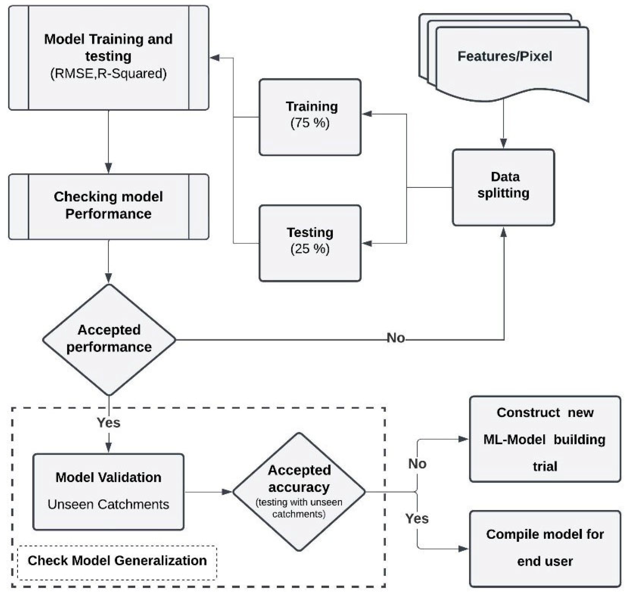
As an initial trial in flood depth prediction model generation, all collected points (pixels) are aggregated to feed the ML algorithm, irrespective of their spatial location within the catchments. This approach harnesses comprehensive data encompassing various points across the catchment area. By integrating clean and scaled input parameters with corresponding target depth outputs, the Trial 01 workflow is shown in Figure 4 and described in the following paragraphs.

The first trial (Trial 01) workflow outlines a step-by-step process for building and validating a model to predict pixel (point) inundation. It begins with collecting features for each pixel, which are then split into training (75%) and testing (25%) datasets. The training dataset is used to train the model, and its performance is evaluated using metrics such as RMSE and R-squared. If the model’s performance is acceptable, it moves on to the testing phase, where it is evaluated again for accuracy using the testing dataset. If the model satisfies the predefined accuracy thresholds, it advances to the validation phase, where its generalizability is assessed using independent, unseen catchments. If the model passes this validation, it is compiled and prepared for deployment to end users. If not, another model-building trial will be conducted. During the building of the RF regression model, the hyperparameters are carefully selected to optimize performance; parameters are tabulated in

Table 6. Selected hyperparameters for the Random Forest (RF) regression model.

Parameter	Value	Description
n_estimators	250	The number of trees in the forest
max_depth	10	The maximum depth of the trees
min_samples_split	2	The minimum number of samples required to split an internal node
min_samples_leaf	1	The minimum number of samples required to be at a leaf node
criterion	‘mse’	Mean Squared Error (MSE), the criterion for measuring the quality
max_features	‘auto’	The maximum number of features considered for splitting a node

.

After training the model, it is evaluated using the testing set. Performance measures such as mean squared error (MSE), root mean squared error (RMSE), and R-squared (R²) are determined to evaluate the model’s precision, as shown in

Table 7. RF model performance indicators for Trial 01.

Performance Indicator	Model: Pixel-Based
	Training	Testing
R2	0.91	0.69
MSE	0.037	0.176
RMSE (m)	0.191	0.42

.

Six catchments in the conterminous United States were selected for model generalization (unseen catchments). Those catchments were calibrated (using flow gauges) for modeling parameters by Soliman et al. (2022) to determine the appropriate CN and “n” [31].

Table 8. Outlet locations and areas for the selected experimental unseen catchments.

Catchment	Outlet Location (UTM-WGS 84)			Catchment Area (km2)
	State	Latitude	Longitude
CA-01	Oregon	43.25261790	−123.0261716	459.47
CA-02	Colorado	39.33415000	−106.5753000	18.73
CA-03	Arizona	34.08282162	−110.9242900	161.02
CA-04	Oklahoma	34.68258000	−98.00893000	90.21
CA-05	Iowa	41.33667771	−92.22240371	67.95
CA-06	St. Louis	39.87476000	−92.02406000	149.27

shows outlet locations and areas for the selected experimental catchments.

The selected calibrated experimental catchments were modeled using the same selected rainfall depth (100 mm/24 h) used in building the regression models, and maximum flood depth values were calculated and extracted. These values were then compared with the predictions from the ML model. The validation results and the estimated performance metrics are shown in

Table 9. Validation results for the unseen experimental catchments (Trial 01).

Validation Catchments	CA_01	CA_02	CA_03	CA_04	CA_05	CA_06
Mean Absolute Error (MAE)	0.409	0.321	0.264	0.118	0.093	0.092
Mean Squared Error (MSE)	0.161	0.059	0.090	0.020	0.013	0.017
Root Mean Squared Error (RMSE)	0.401	0.243	0.300	0.143	0.117	0.131
Nash–Sutcliffe Efficiency (NSE)	0.43	0.38	0.56	0.62	0.72	0.75
Coefficient of Determination (R2)	44%	40%	57%	65%	73%	75%

.

The performance metrics across the six catchments for the model (Trial 01) indicate that the model generally performs well; however, the lower NSE and R² values for CA_01 and CA_02 suggest that the model’s performance is less satisfactory for some unseen catchments (this is due to the fact that spatial variations of physical internal pixel relationships were not well captured in the first trial). This variation in performance metrics highlights the model’s inconsistent ability to generalize new data. A second trial will be conducted to enhance model performance and generalization.

3.6.2. Trial 2: Clustered Pixel-Based Depth Regression Model

To enhance flood depth prediction accuracy, this study introduces Trial 02, an improved modeling approach that addresses limitations in the initial trial. Recognizing that the first model overlooked spatial variations in pixel-level physical relationships—leading to potential confusion, the researchers propose a hybrid method. This combines:

• Unsupervised clustering to pre-group pixels (clusters) by physical characteristics;
• Supervised regression (RM) for refined prediction.

By explicitly accounting for spatial dependencies and boundary conditions, the hybrid framework aims to significantly boost predictive performance.

A.

Unsupervised Clustering

The K-means algorithm partitions data points into K clusters based on similarity. The process begins by randomly initializing K centroids, then iteratively:

• Assign points to the nearest centroids;
• Recalculates centroids as cluster means until convergence (no centroid movement) or max iterations.

Selecting the optimal number of clusters is essential, as an inappropriate K can lead to poor cluster assignments. The most popular methods for determining the optimal K are the Elbow Method and the Silhouette Score Method. The Silhouette Score Method indicates that the clustering model with five clusters (K = 5) provides the highest average silhouette score (see Appendix A,

Table A4. Silhouette score calculated versus the selected number of clusters.

No. of Clusters	Silhouette Score	No. of Clusters	Silhouette Score
K = 3	0.481	K = 6	0.468
K = 4	0.482	K = 7	0.462
K = 5	0.486

) and, hence, is identified as the optimal number of clusters for the dataset under investigation.

B.

Flood Depth Regression Models

Upon completion of the data clustering process using the K-means method, all data points are subjected to filtering using the developed K-means model. Each data point is then assigned a unique cluster number identifier based on its location within a specific cluster. Subsequently, data within each cluster are utilized to train an RF model that can predict the expected flood depth. RF models’ training and testing R² and MSE values are presented in

Table 10. Performance for model training and testing metric values—Trial 02.

Indicator	Clustered Pixel-Based Depth Regression Model (Trial 2)
	Cluster/Model-01		Cluster/Model-02		Cluster/Model-03		Cluster/Model-04		Cluster/Model-05		Overall Performance
	Training	Testing	Training	Testing	Training	Testing	Training	Testing	Training	Testing	Training	Testing
R2 (%)	94	74	93	67	95	74	94	81	95	87	95	75
MSE	0.01	0.05	0.01	0.05	0.01	0.06	0.01	0.05	0.01	0.03	0.01	0.05
RMSE (m)	0.1	0.274	0.1	0.29	0.1	0.245	0.165	0.324	0.1	0.173	0.14	0.29

.

The performance metrics indicate that the models perform well during training, with high R² values (ranging from 93% to 95%) and low MSE and RMSE values. However, the testing results show more variability, with R² values ranging from 67% to 87%. This suggests the model’s ability to generalize new, unseen data varies across different clusters. Clusters 04 and 05 show the highest R² values during testing (81% and 87%, respectively), indicating strong model verification. Overall, the cumulative model’s performance is better than the initial trial (Trial 01). The hybrid model (Trial 02), integrating clustering and regression, was tested on six experimental catchments to assess its generalization capability. The results (

Table 11. Validation results for the unseen experimental catchments (Trial 02).

Validation Catchments	CA_01	CA_02	CA_03	CA_04	CA_05	CA_06
Mean Absolute Error (MAE)	0.323	0.253	0.209	0.093	0.073	0.073
Mean Squared Error (MSE)	0.136	0.050	0.076	0.017	0.012	0.015
Root Mean Squared Error (RMSE)	0.3693	0.2232	0.2765	0.1315	0.1074	0.1206
Nash–Sutcliffe Efficiency (NSE)	0.467	0.413	0.609	0.674	0.783	0.815
Coefficient of Determination (R2)	48%	45%	60%	71%	78%	81%

) revealed poor performance for unseen catchments, particularly CA-01 and CA-02, evidenced by low R² values. This limitation stems from the model’s inability to fully capture spatial heterogeneity and nuanced pixel-level physical relationships in these catchments. Given these shortcomings, further refinement (e.g., enhanced spatial feature engineering or adaptive clustering) is necessary to improve generalization across diverse hydrological conditions.

3.6.3. Trial 03: Clustered Catchment-Based Depth Regression Model

A catchment-based approach was explored as a refined trial to incorporate hidden physical relationships and spatial location parameters for improved model performance and generalization. This involved integrating an unsupervised clustering model with catchment parameters, represented by indicators such as mode, mean, and median. Subsequently, regression models were applied to each cluster as in Trial 2, grouping catchments based on shared characteristics. This method aims to enhance the model’s ability to capture nuanced spatial dependencies and optimize predictions tailored to specific catchment conditions.

The process begins with data aggregation from various catchments. These data are then aggregated to calculate features per pixel within each catchment, followed by computing statistical features, resulting in mean, mode, and median values for each feature set in each catchment. These descriptive feature values are crucial for building an unsupervised clustering model. Using the K-means algorithm, data were clustered based on mean, mode, and median values to analyze descriptive feature dependencies for flood depth prediction. The optimal number of clusters (n) was determined using the same methodology applied in Trial 02. The optimal cluster counts were determined as five, three, and three for mean, mode, and median values, respectively. Then, separate regression models (RM-01 to RM-n) were trained for each cluster grouping to enhance predictive accuracy and model robustness.

Table 12. Performance measures for clustered catchment-based depth regression models based on different statistical parametric features (mean, mode, and median).

Model Type	Number of Clusters	R2 (Training)	R2 (Testing)	MSE (Training)	MSE (Testing)	RMSE (m) (Training)	RMSE (m) (Testing)
Mean-based	5	0.97	0.83	0.01	0.04	0.1	0.21
Mode-based	3	0.64	0.51	0.040	0.122	0.225	0.389
Median-based	3	0.71	0.64	0.020	0.082	0.143	0.286

outlines the training and testing performance of clustered catchment-based depth regression models. These results highlight the mean-based models’ superiority in the training and testing phases compared with the other types.

For further verification of the selected K value for the mean-based models, the sensitivity analysis revealed a clear trade-off between training accuracy and generalization. Increasing K from 3 to 5 improved training (R² from 64% to 97%) and testing (R² from 51% to 83%), reflecting better spatial representation. Beyond K = 5, testing accuracy declined (R² down to 78% and 72%), indicating overfitting (

Table 13. Sensitivity analysis of the number of clusters (K) using silhouette score, R², and RMSE for training and testing—Trial 03.

No. of Clusters (K)	Silhouette Score	R2 (Training) %	R2 (Testing) %	RMSE (Training) (m)	RMSE (Testing) (m)
3	0.481	64%	51%	0.225	0.389
4	0.482	85%	70%	0.150	0.280
5	0.486	97%	83%	0.100	0.210
6	0.468	98%	78%	0.090	0.250
7	0.462	98%	72%	0.080	0.300

). Therefore, K = 5 was chosen as it offers the best balance, supported by the highest silhouette score (0.486).

For each cluster in the selected model (man-based) identified by the K-means model, a separate supervised regression model (labeled RM-01 to RM-5) is trained to predict flood depths. The performance of each regression model is evaluated using metrics such as root mean squared error (RMSE) and R-squared (see

Table 14. Performance for models’ training and testing metric values—Trial 03.

Indicator	Clustering/Catchments Based Model-Mean (Parameters)
	Cluster/Model-01		Cluster/Model-02		Cluster/Model-03		Cluster/Model-04		Cluster/Model-05		Overall Performance
	Training	Testing	Training	Testing	Training	Testing	Training	Testing	training	Testing	Training	Testing
R2 (%)	98	86	98	84	96	83	97	82	98	76	97	83
MSE	0.01	0.03	0.01	0.02	0.01	0.07	0.01	0.04	0.01	0.08	0.01	0.04
RMSE (m)	0.10	0.17	0.10	0.14	0.10	0.26	0.10	0.20	0.09	0.28	0.10	0.21

). If the models demonstrate acceptable performance, the workflow proceeds to the next stage; otherwise, adjustments are made to improve model accuracy.

The evaluated models were subsequently tested on a set of unseen catchments to assess their generalization capabilities. As presented in

Table 15. Validation results for the unseen experimental catchments (Trial 03).

Validation Catchments	CA_01	CA_02	CA_03	CA_04	CA_05	CA_06
Cluster/Model	Cluster 05	Cluster 05	Cluster 03	Cluster 02	Cluster 01	Cluster 01
Mean Absolute Error (MAE)	0.176	0.122	0.148	0.073	0.067	0.069
Mean Squared Error (MSE)	0.082	0.035	0.060	0.019	0.011	0.014
Root Mean Squared Error (RMSE)	0.286	0.187	0.245	0.139	0.105	0.117
Nash–Sutcliffe Efficiency (NSE)	0.845	0.639	0.843	0.666	0.891	0.920
Coefficient of Determination (R2)	86%	67%	86%	70%	90%	92%

, the models developed in Trial 03 demonstrated acceptable predictive performance, validating their applicability in new settings. Based on the parameter sensitivity analysis (Section 3.4.1), four geospatial parameters (Distance to Stream (DTS), Elevation (ELV), SINK, and FACV) were identified as the most influential inputs affecting model accuracy. Guided by these parameters, the unseen catchments were assigned to their most representative clusters using model outputs. Notably, CA_01 and CA_02, which showed the lowest validation performance, were associated with Cluster 05—identified by the K-means clustering model. As shown in Table 14, Cluster 05 had the weakest test performance (R² = 76%, RMSE = 0.28 m), aligning with the increased prediction error observed in those catchments. This outcome highlights some limitations in generalization over regions characterized by flat terrain, low elevation variability, high sink density, and greater distances to streams. Nevertheless, the model maintained robust performance across the majority of validation catchments and demonstrated strong adaptability overall. It is therefore recommended to increase the representation of such underrepresented geospatial conditions within the training dataset to further enhance reliability. With these considerations in mind, and after passing all generalizability checks across varied terrain conditions, the model is considered sufficiently mature and has been compiled for deployment to the end user.

3.6.4. Summary of Regression Model Improvement Path

The model development followed a structured progression across three regression trials, each addressing key limitations identified in the previous approach. Trial 1 adopted a point-based regression using all pixel data without spatial clustering. While this approach served as a baseline, it demonstrated limited generalization performance. In Trial 2, spatial variability was introduced through K-means clustering of pixel-level features, resulting in better boundary condition handling and improved accuracy. Trial 3 extended this concept by applying clustering at the catchment level using statistical descriptors (mean, mode, and median), which allowed the model to capture broader hydrological dependencies across space. This final design achieved the best overall performance. As summarized in

Table 16. Summary of regression model trials and performance metrics.

Trial	Model Type	Clustering Strategy	Training R2 (%)	Testing R2 (%)	Validation (Unseen Catchments) R2 (Range)	RMSE (Testing) (m)	Key Notes
1	Pixel-Based Regression	None	91	69	44–75%	0.42	Baseline; poor spatial representation
2	Clustered Pixel-Based Regression	K-means on physical pixel features	95	75	45–81%	0.29	Improved boundary handling and clustering
3	Clustered Catchment-Based Regression	K-means on catchment parameters (mean, mode, and median)	97	83	67–92%	0.21	Best performance and generalization

, trial 3 reflects a clear increase in both training and testing R² values, alongside decreasing RMSE and improved validation across unseen catchments.

3.6.5. Model Implementation’s Capability and Application

The subsequent section evaluates the developed models’ performance by systematically comparing hydrodynamic model outputs with machine learning-based predictions. Benchmarking the predictive ML model against HEC-RAS 6.3 across six reserved, unseen catchments demonstrated substantial gains in computational efficiency and time savings.

Based on a Windows 10 workstation with a Ryzen™ 7 4800H CPU (Advanced Micro Devices, Inc. [AMD], Santa Clara, CA, USA), 16 GB RAM, and a GTX 1660 Ti GPU, parallel processing was utilized during data preprocessing and model inference stages through Python’s multiprocessing library and scikit-learn’s n_jobs parameter, enabling concurrent processing of spatial tiles and model iterations. This setup provided a practical and cost-effective environment for significantly accelerating computation.

Table 17. Benchmarking simulation time results between HEC-RAS 6.3 simulations and the predictive ML model across six unseen catchments.

Catchment	Area (km2)	HEC-RAS Simulation Time (h)	ML Parameter Extraction Time (h)	ML Prediction Time (h)	Total ML Runtime (h)
CA-01	459.47	22.46	0.07	0.03	0.10
CA-02	18.73	0.92	0.00	0.03	0.04
CA-03	161.02	7.87	0.02	0.03	0.06
CA-04	90.21	4.41	0.01	0.03	0.05
CA-05	67.95	3.32	0.01	0.03	0.04
CA-06	149.27	7.30	0.02	0.03	0.05

clearly shows these advantages, highlighting the model’s potential for near-real-time flood forecasting. The ML model’s ability to deliver near-instant results without sacrificing accuracy underscores its scalability. HEC-RAS simulations used high-resolution 2D modeling with conservative adaptive time stepping and took between 0.92 and 22.46 h per catchment (see Table 17). In contrast, the ML model completed predictions (including parameter extraction) in less than 0.1 h (6 min) per catchment. This represents a speed-up factor of up to 225. This significant time reduction is critical for operational decision-making, reducing the computation cost, and establishing a foundation for effective flood early warning systems (FEWS). By enabling near-real-time flood forecasting, the approach enhances preparedness and emergency response capabilities—key factors in mitigating flood disaster impacts. Furthermore, the consistent ML performance across catchments of varying sizes indicates robustness. The reduced computational demand allows for rapid scenario testing and deployment in resource-limited settings. This positions the ML model as a practical complement to traditional hydrodynamic tools.

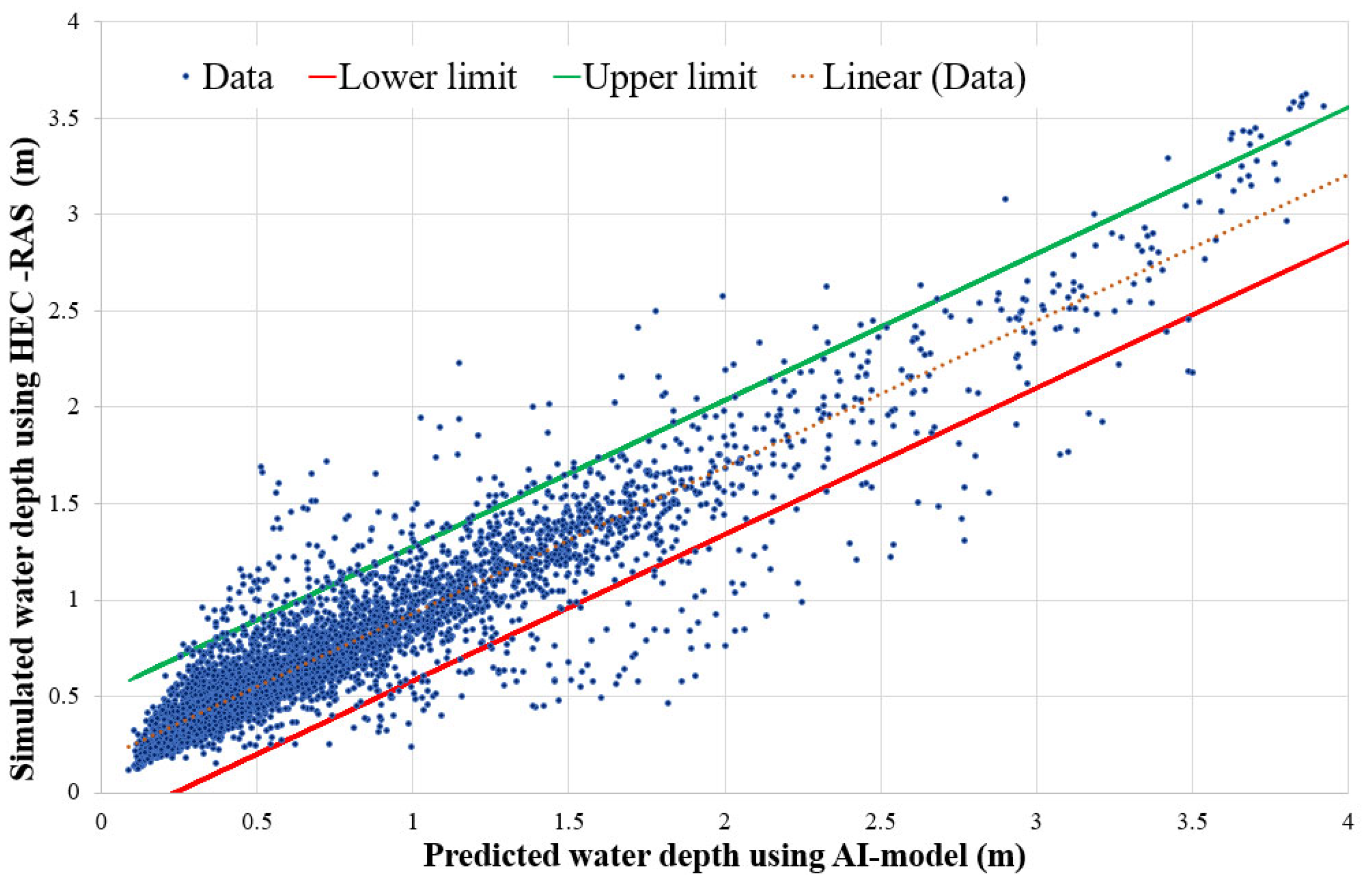
Given the critical importance of uncertainty quantification in flood depth estimation, particularly for model transfer to ungauged catchments, 95% confidence intervals (α = 0.05) were developed to assess prediction reliability. For one of the experimental catchments selected (CA-03) as an example, a detailed comparison was conducted between the ML model predictions and HEC-RAS simulation outputs with a 95% confidence interval. Figure 5 shows the lower and upper limits and highlights the good correlation and accuracy between predicted and actual flood depths with a 95% confidence limit.

The discrepancies observed in Figure 5 may stem from inaccuracies in these input data or limitations in the underlying hydrodynamic assumptions.

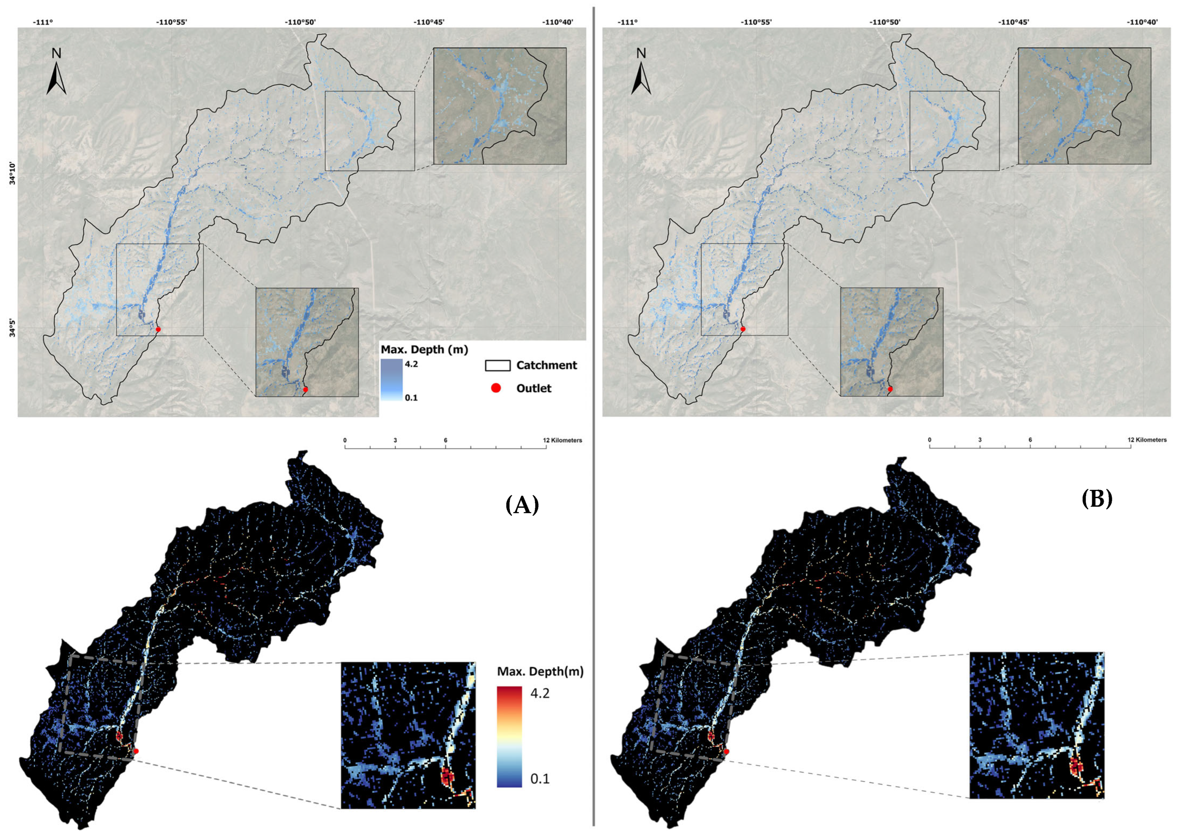
Figure 6 presents the spatial distribution of flood depths using raster maps overlaid on satellite imagery, allowing a visual comparison of the two modeling approaches. This evaluation emphasizes the practical strengths and limitations of applying ML-based models in real-world flood forecasting. The figure also demonstrates the model’s effectiveness in capturing inundated cells. Recalling the classification model as detailed in Section 3.5.2, the performance of the inundation detection component, particularly the recall metric, indicates a reasonable capability to identify inundated cells. However, the Random Forest (RF) pixel-based classification model tends to produce several false positives—pixels incorrectly classified as inundated when they are, in fact, dry.

These false positives introduce a systematic issue in the subsequent regression-based depth estimation model. Specifically, falsely inundated pixels are assigned to very low or near-zero depth values, which adversely affects the overall accuracy of depth predictions. This phenomenon is particularly critical in contexts where the primary objective is to reliably estimate maximum water depth for risk assessment or early warning systems.

The depth-related errors are further illustrated in Figure 5, which displays the R² values, confidence intervals (CI), and associated regression errors of the ML models, highlighting both strengths and limitations in depth prediction accuracy. These results form a foundational step toward early flood warning systems and offer the possibility for future expansion to include flow velocity and other key parameters essential for building comprehensive hazard and risk models.

4. Discussion

This study presented a detailed methodology for developing a global flood depth prediction model by leveraging machine learning algorithms and extensive hydrodynamic data. The data preparation process involved integrating high-resolution datasets with global covers, such as LULC 2020-ESRI, AW3D30 DEM, and HYSOGs 250m, which were essential for accurate flood modeling. Numerical modeling using 2D hydrodynamic simulations provided maximum flood depth values, and spatial and parametric analyses were performed to extract and refine features for model training. A crucial step in this methodology was the selection of 45 catchment areas globally distributed, ensuring a wide variability in flood-driving parameters. These catchments were delineated and analyzed based on elevation, land use, land cover, and soil type, providing a comprehensive dataset for model training and validation. This study developed an RF classification model to predict pixel inundation, which was evaluated using a confusion matrix. The classification model demonstrated strong performance, with an accuracy of 86% and 84% and an F1-score of 0.83 and 0.81 for the entire and test datasets, respectively (see Table 3). These results highlight the model’s effectiveness in distinguishing between inundated and non-inundated pixels.

A comprehensive evaluation was conducted of six machine learning algorithms (ANN, CNN, RNN, LSTM, Random Forest, and XGBoost) for pixel-level maximum flood depth prediction. This comparative analysis served as the foundation for selecting the optimal algorithm for the dataset. Among all models tested, the Random Forest algorithm demonstrated superior generalization performance, achieving the highest test R² of 0.69 and the lowest test RMSE of 0.483 m (see Table 5). These results indicate that the Random Forest approach provides the most reliable predictive accuracy for flood depth estimation in this study.

The methodology also included developing and evaluating three regression models (trials): a pixel-based regression model, a clustered pixel-based regression model, and a clustered catchment-based regression model. In Trial 01, the pixel-based depth regression model achieved R² values of 91% for training and 69% for testing, with validation on unseen catchments yielding an average NSE of 0.55 and R² of 60%. Trial 02 introduced K-means clustering to group pixels based on physical characteristics, resulting in an overall testing R² of 75% and improved validation metrics, with an average NSE of 0.69 and R² of 66% across validation catchments. Trial 03 further advanced the methodology by incorporating catchment-specific parameters for clustering, achieving a training R² of 97% and a testing R² of 83%. The validation results for this model indicated high accuracy, with an average NSE of 0.79 and an R² of 82%.

The capabilities of the developed ML model were evaluated for flood depth estimation using unseen catchment benchmarks. The developed machine learning model generates flood depth predictions in just 6 min—a dramatic improvement over traditional HEC-RAS simulations, which typically require hours to complete. This rapid prediction capability is critical for operational flood warning systems, enabling timely emergency responses. The ML model provides flood depth predictions with statistically robust 95% confidence intervals (Figure 5), ensuring reliable uncertainty quantification for decision-making. Comparative analysis demonstrates an excellent correspondence between modeled and observed inundation maps, validating the ML model’s spatial prediction capabilities. The model’s combination of speed (sub-10 min predictions) and reliability (quantified uncertainty) represents a significant advancement for operational flood forecasting systems. While this study demonstrates the potential of machine learning models to surrogate hydrodynamic simulations and achieve significant computational efficiency gains (over 225×), it is important to note that the models are trained on HEC-RAS outputs, which, although derived from well-calibrated baseline scenarios (Soliman et al., 2022) [31], may not fully represent real-world flood behavior. This dependency represents a key limitation. To address this, future research should include validation using observed flood data or satellite-derived flood extents to improve real-world applicability. Furthermore, future work should explore the use of higher-resolution data, advanced clustering algorithms, and the incorporation of actual rainfall event characteristics (depth and duration) along with real-time data integration to enhance model accuracy and scalability for global flood risk management and mitigation.

5. Conclusions

This study demonstrated significant advancements in developing a scalable modeling framework with potential for global generalization of flood depth prediction models using machine learning models. This study initiated with the careful selection of 45 geographically diverse catchments to capture wide variations in key flood-influencing factors, followed by comprehensive data collection of all relevant hydrological parameters. Six prominent machine learning approaches—including Artificial Neural Networks (ANNs), Convolutional Neural Networks (CNNs), Recurrent Neural Networks (RNNs), Long Short-Term Memory networks (LSTMs), Random Forest (RF), and XGBoost—were rigorously evaluated for their pixel-scale flood depth prediction capabilities. Through systematic comparison, the Random Forest algorithm demonstrated superior performance, establishing itself as the most effective model for flood forecasting applications.

This study systematically evaluated three progressive modeling approaches: (1) a basic pixel-based regression (Trial 1), (2) a clustered pixel-based depth regression (Trial 2), and (3) a clustered catchment-based depth regression (Trial 3). Trial 3 emerged as the superior model, demonstrating exceptional predictive accuracy with a training R² of 0.97 and a testing R² of 0.83. When validated on six unseen catchments, the developed ML model maintained strong performance, achieving an average Nash–Sutcliffe Efficiency (NSE) of 0.79 and R² of 0.82, confirming its reliability for flood depth prediction in ungauged basins. The main advantages of the developed ML model can be summarized as follows:

• Computational Efficiency

  ○

  Achieves complete flood depth spatial distribution predictions within 6 min;

  ○

  Provides a 225× speed improvement over HEC-RAS 6.3 simulations;

  ○

  Represents a 90–95% time reduction compared with HEC-RAS simulations;

  ○

  Enables the foundation for flood early warning system implementation.

• Prediction Accuracy

  ○

  Delivers estimates with statistically robust 95% confidence intervals (Figure 5);

  ○

  Shows strong agreement with the HEC-RAS 6.3 benchmark depth maps (Figure 6).

• Operational Value

  ○

  Establishes a foundation for emergency response decision-making;

  ○

  Maintains accuracy while dramatically reducing computational requirements.

Finally, these advancements establish the developed ML model as both a rapid and reliable alternative to conventional hydrodynamic modeling for a scalable modeling framework for flood depth prediction.

References

1. Quintero, F.; Mantilla, R.; Anderson, C.; Claman, D.; Krajewski, W. Assessment of changes in flood frequency due to the effects of climate change: Implications for engineering design. Hydrology 2018, 5, 19. [Google Scholar] [CrossRef]
2. Masson-Delmotte, V.; Zhai, P.; Pirani, A.; Connors, S.L.; Péan, C.; Berger, S.; Caud, N.; Chen, Y.; Goldfarb, L.; Gomis, M.I.; et al. Climate Change 2021: The Physical Science Basis. Contribution of Working Group I to the Sixth Assessment Report of the Intergovernmental Panel on Climate Change; Cambridge University Press: Cambridge, UK, 2021; p. 2391. [Google Scholar]
3. Lendering, K.T.; Jonkman, S.N.; Kok, M. Effectiveness of emergency measures for flood prevention. J. Flood Risk Manag. 2016, 9, 320–334. [Google Scholar] [CrossRef]
4. Perera, D.; Seidou, O.; Agnihotri, J.; Mehmood, H.; Rasmy, M. Challenges and Technical Advances in Flood Early Warning Systems (FEWSs). In Flood Impact Mitigation and Resilience Enhancement; Huang, G., Ed.; IntechOpen: London, UK, 2020. [Google Scholar]
5. Cheong, T.S.; Kim, S.; Koo, K.M. Development of measured hydrodynamic information-based flood early warning system for small streams. Water Res. 2024, 263, 122159. [Google Scholar] [CrossRef] [PubMed]
6. Shang, C.; Yang, F.; Huang, D.; Lyu, W. Data-driven soft sensor development based on deep learning technique. J. Process Control 2014, 24, 223–233. [Google Scholar] [CrossRef]
7. Mitchell, T.M. Does machine learning really work? AI Mag. 1997, 18, 11. [Google Scholar]
8. LeCun, Y.; Bengio, Y.; Hinton, G. Deep learning. Nature 2015, 521, 436–444. [Google Scholar] [CrossRef]
9. Bentivoglio, R.; Isufi, E.; Jonkman, S.N.; Taormina, R. Deep learning methods for flood mapping: A review of existing applications and future research directions. Hydrol. Earth Syst. Sci. 2022, 26, 4345–4378. [Google Scholar] [CrossRef]
10. Horritt, M.S.; Bates, P.D. Evaluation of 1D and 2D numerical models for predicting river flood inundation. J. Hydrol. 2002, 268, 87–99. [Google Scholar] [CrossRef]
11. Teng, J.; Jakeman, A.J.; Vaze, J.; Croke, B.F.; Dutta, D.; Kim, S.J. Flood inundation modelling: A review of methods, recent advances and uncertainty analysis. Environ. Model. Softw. 2017, 90, 201–216. [Google Scholar] [CrossRef]
12. Costabile, P.; Costanzo, C.; Macchione, F. Performances and limitations of the diffusive approximation of the 2-D shallow water equations for flood simulation in urban and rural areas. Appl. Numer. Math. 2017, 116, 141–156. [Google Scholar] [CrossRef]
13. Tayefi, V.; Lane, S.N.; Hardy, R.J.; Yu, D. A comparison of one- and two-dimensional approaches to modelling flood inundation over complex upland floodplains. Hydrol. Process. 2007, 21, 3190–3202. [Google Scholar] [CrossRef]
14. Bates, P.D.; De Roo, A.P.J. A simple raster-based model for flood inundation simulation. J. Hydrol. 2000, 236, 54–77. [Google Scholar] [CrossRef]
15. Merwade, V.; Cook, A.; Coonrod, J. GIS techniques for creating river terrain models for hydrodynamic modeling and flood inundation mapping. Environ. Model. Softw. 2008, 23, 1300–1311. [Google Scholar] [CrossRef]
16. Zhang, S.; Xia, Z.; Yuan, R.; Jiang, X. Parallel computation of a dam-break flow model using OpenMP on a multi-core computer. J. Hydrol. 2014, 512, 126–133. [Google Scholar] [CrossRef]
17. Ming, X.; Liang, Q.; Xia, X.; Li, D.; Fowler, H.J. Real-time flood forecasting based on a high-performance 2-D hydrodynamic model and numerical weather predictions. Water Resour. Res. 2020, 56, e2019WR025583. [Google Scholar] [CrossRef]
18. Costache, R.; Pal, S.C.; Pande, C.B.; Islam, A.R.M.T.; Alshehri, F.; Abdo, H.G. Flood mapping based on novel ensemble modeling involving deep learning, Harris Hawk optimization algorithm, and stacking-based machine learning. Appl. Water Sci. 2024, 14, 78. [Google Scholar] [CrossRef]
19. Dai, W.; Tang, Y.; Liao, N.; Zou, S.; Cai, Z. Urban flood prediction using ensemble artificial neural network: An investigation on improving model uncertainty. Appl. Water Sci. 2024, 14, 144. [Google Scholar] [CrossRef]
20. Seleem, O.; Ayzel, G.; Bronstert, A.; Heistermann, M. Transferability of data-driven models to predict urban pluvial flood water depth in Berlin, Germany. Nat. Hazards Earth Syst. Sci. 2022, 23, 809–831. [Google Scholar] [CrossRef]
21. Jang, J.-S.R. ANFIS: Adaptive Network-Based Fuzzy Inference System. IEEE Trans. Syst. Man Cybern. 1993, 23, 665–685. [Google Scholar] [CrossRef]
22. Esmaeili-Gisavandani, H.; Zarei, H.; Fadaei Tehrani, M.R. Regional flood frequency analysis using data-driven models (M5, random forest, and ANFIS) and a multivariate regression method in ungauged catchments. Appl. Water Sci. 2023, 13, 139. [Google Scholar] [CrossRef]
23. Balestra, F.; Del Vecchio, M.; Pirone, D.; Pedone, M.A.; Spina, D.; Manfreda, S.; Menduni, G.; Bignami, D.F. Flood Susceptibility Mapping Using a Deep Neural Network Model: The Case Study of Southern Italy. Environ. Sci. Proc. 2022, 21, 36. [Google Scholar]
24. Chen, W.; Hong, H.; Li, S.; Shahabi, H.; Wang, Y.; Wang, X.; Ahmad, B.B. Flood Susceptibility Modelling Using a Novel Hybrid Approach of Reduced-Error Pruning Trees with Bagging and Random Subspace Ensembles. J. Hydrol. 2019, 575, 864–873. [Google Scholar] [CrossRef]
25. Xie, S.; Wu, W.; Mooser, S.; Wang, Q.J.; Nathan, R.; Huang, Y. Artificial neural network-based hybrid modeling approach for flood inundation modeling. J. Hydrol. 2021, 592, 125605. [Google Scholar] [CrossRef]
26. Šmuc, T.; Gamberger, D.; Krstačić, G. Combining unsupervised and supervised machine learning in analysis of the CHD patient database. In Artificial Intelligence in Medicine, Proceedings of the AIME 2001, Cascais, Portugal, 1–4 July 2001; Springer: Berlin/Heidelberg, Germany, 2001; pp. 109–112. [Google Scholar]
27. Ran, J.; Ji, Y.; Tang, B. A semi-supervised learning approach to IEEE 802.11 network anomaly detection. In Proceedings of the 2019 IEEE 89th Vehicular Technology Conference (VTC2019-Spring), Kuala Lumpur, Malaysia, 28 April–1 May 2019; pp. 1–5. [Google Scholar]
28. Wang, J.; Biljecki, F. Unsupervised machine learning in urban studies: A systematic review of applications. Cities 2022, 129, 103925. [Google Scholar] [CrossRef]
29. Solomon, S.; Qin, D.; Manning, M.; Chen, Z.; Marquis, M.; Averyt, K.B.; Tignor, M.; Miller, H.L. Model Evaluation. In Climate Change 2007: The Physical Science Basis. Contribution of Working Group I to the Fourth Assessment Report of the Intergovernmental Panel on Climate Change; Cambridge University Press: Cambridge, UK, 2007; pp. 600–647. [Google Scholar]
30. Tadono, T.; Ishida, H.; Oda, F.; Naito, S.; Minakawa, K.; Iwamoto, H. Precise global DEM generation by ALOS PRISM. ISPRS Ann. Photogramm. Remote Sens. Spat. Inf. Sci. 2014, II, 71–76. [Google Scholar] [CrossRef]
31. Soliman, M.; Morsy, M.M.; Radwan, H.G. Assessment of implementing Land Use/Land Cover LULC 2020-ESRI Global Maps in 2D flood modeling application. Water 2022, 14, 3963. [Google Scholar] [CrossRef]
32. Karra, K.; Kontgis, C.; Statman-Weil, Z.; Mazzariello, J.C.; Mathis, M.; Brumby, S.P. Global land use/land cover with Sentinel 2 and deep learning. In Proceedings of the 2021 IEEE International Geoscience and Remote Sensing Symposium IGARSS, Brussels, Belgium, 11–16 July 2021; pp. 4704–4707. [Google Scholar]
33. Ross, C.W.; Prihodko, L.; Anchang, J.; Kumar, S.; Ji, W.; Hanan, N.P. Global Hydrologic Soil Groups (HYSOGs250m) for Curve Number-Based Runoff Modeling. Sci. Data 2018, 5, 180091. [Google Scholar] [CrossRef]
34. Brunner, G.W. HEC-RAS River Analysis System 2D Modeling User’s Manual; U.S. Army Corps of Engineers—Hydrologic Engineering Center: Washington, DC, USA, 2016; pp. 1–171. [Google Scholar]
35. Cronshey, R. Urban Hydrology for Small Watersheds; U.S. Department of Agriculture, Soil Conservation Service, Engineering Division: Washington, DC, USA, 1986. [Google Scholar]
36. David, A.; Schmalz, B. A systematic analysis of the interaction between rain-on-grid simulations and spatial resolution in 2D hydrodynamic modeling. Water 2021, 13, 2346. [Google Scholar] [CrossRef]
37. Quiroga, V.M.; Kure, S.; Udo, K.; Manoa, A. Application of 2D numerical simulation for the analysis of the February 2014 Bolivian Amazonia flood: Application of the new HEC-RAS version 5. Ribagua 2016, 3, 25–33. [Google Scholar] [CrossRef]
38. SCS, USDA. National Engineering Handbook, Section 4: Hydrology; U.S. Soil Conservation Service, USDA: Washington, DC, USA, 1985; Available online: https://archive.org/download/CAT71334647003/CAT71334647003.pdf (accessed on 10 March 2023).
39. Costabile, P.; Costanzo, C.; Ferraro, D.; Macchione, F.; Petaccia, G. Performances of the new HEC-RAS version 5 for 2-D hydrodynamic-based rainfall-runoff simulations at basin scale: Comparison with a state-of-the-art model. Water 2020, 12, 2326. [Google Scholar] [CrossRef]
40. Savitri, Y.R.; Kakimoto, R.; Anwar, N.; Wardoyo, W.; Suryani, E. Reliability of 2D hydrodynamic model on flood inundation analysis. GEOMATE J. 2021, 21, 65–71. [Google Scholar] [CrossRef]
41. Hariri, S.; Weill, S.; Gustedt, J.; Charpentier, I. A balanced watershed decomposition method for rain-on-grid simulations in HEC-RAS. J. Hydroinform. 2022, 24, 315–332. [Google Scholar] [CrossRef]
42. Zeiger, S.J.; Hubbart, J.A. Measuring and modeling event-based environmental flows: An assessment of HEC-RAS 2D rain-on-grid simulations. J. Environ. Manag. 2021, 285, 112125. [Google Scholar] [CrossRef] [PubMed]
43. Naaman, M. On the tight constant in the multivariate Dvoretzky–Kiefer–Wolfowitz inequality. Stat. Probab. Lett. 2021, 173, 109088. [Google Scholar] [CrossRef]
44. Moore, D.S.; McCabe, G.P.; Craig, B.A. Chapter 2: Descriptive Statistics. In Introduction to the Practice of Statistics, 8th ed.; W.H. Freeman: New York, NY, USA, 2014; pp. 23–65. [Google Scholar]
45. Ben-Gal, I. Outlier Detection. In Data Mining and Knowledge Discovery Handbook; Maimon, O., Rokach, L., Eds.; Springer: Boston, MA, USA, 2005. [Google Scholar]
46. Aggarwal, C.C. Chapter 2: Statistical Methods for Outlier Detection. In Outlier Analysis, 2nd ed.; Springer: Cham, Switzerland, 2017; pp. 9–45. [Google Scholar]
47. Jalayer, F.; De Risi, R.; De Paola, F.; Giugni, M.; Manfredi, G.; Gasparini, P.; Topa, M.E.; Yonas, N.; Yeshitela, K.; Nebebe, A.; et al. Probabilistic GIS-based method for delineation of urban flooding risk hotspots. Nat. Hazards 2014, 73, 975–1001. [Google Scholar] [CrossRef]
48. He, H.; Garcia, E.A. Learning from imbalanced data. IEEE Trans. Knowl. Data Eng. 2009, 21, 1263–1284. [Google Scholar] [CrossRef]
49. Zhao, G.; Pang, B.; Xu, Z.; Peng, D.; Zuo, D. Urban flood susceptibility assessment based on convolutional neural networks. J. Hydrol. 2020, 590, 125235. [Google Scholar] [CrossRef]
50. Löwe, R.; Böhm, J.; Jensen, D.G.; Leandro, J.; Rasmussen, S.H. U-FLOOD—Topographic deep learning for predicting urban pluvial flood water depth. J. Hydrol. 2021, 603, 126898. [Google Scholar] [CrossRef]
51. Rahmati, O.; Pourghasemi, H.R.; Zeinivand, H. Flood susceptibility mapping using frequency ratio and weights-of-evidence models in the Golastan Province, Iran. Geocarto Int. 2016, 31, 42–70. [Google Scholar] [CrossRef]
52. Inyang, U.G.; Akpan, E.E.; Akinyokun, O.C. A hybrid machine learning approach for flood risk assessment and classification. Int. J. Comput. Intell. Appl. 2020, 19, 2050012. [Google Scholar] [CrossRef]
53. Vinutha, H.P.; Poornima, B.; Sagar, B.M. Detection of Outliers Using Interquartile Range Technique from Intrusion Dataset. In Information and Decision Sciences; Advances in Intelligent Systems and Computing; Satapathy, S., Tavares, J., Bhateja, V., Mohanty, J., Eds.; Springer: Singapore, 2018; Volume 701. [Google Scholar]
54. Wieland, M.; Martinis, S. A modular processing chain for automated flood monitoring from multi-spectral satellite data. Remote Sens. 2019, 11, 2330. [Google Scholar] [CrossRef]
55. Farhadi, H.; Najafzadeh, M. Flood risk mapping by remote sensing data and Random Forest technique. Water 2021, 13, 3115. [Google Scholar] [CrossRef]
56. Chicco, D.; Jurman, G. The advantages of the Matthews correlation coefficient (MCC) over F1 score and accuracy in binary classification evaluation. BMC Genom. 2020, 21, 6. [Google Scholar] [CrossRef] [PubMed]
57. Alpaydin, E. Introduction to Machine Learning; MIT Press: Cambridge, MA, USA, 2020. [Google Scholar]
Figure 1. Research general methodology workflow.
Hydrology 12 00223 g001
Figure 2. Selected catchment locations are projected onto a global satellite image, demonstrating the geographical distribution of study areas.
Hydrology 12 00223 g002
Figure 3. Predictive feature importance resulted from RF.
Hydrology 12 00223 g003
Figure 4. Workflow for the first trial building a point-based depth regression model (Trial #01).
Hydrology 12 00223 g004
Figure 5. Regression and 95% confidence interval between actual and predicted values of flood depth from HEC-RAS and ML model (CA-03).
Hydrology 12 00223 g005
Figure 6. Spatial distribution of flood depths (A) simulated by HEC-RAS and (B) predicted by the ML model (CA-03).
Hydrology 12 00223 g006