Article

Evaluation and Bias Correction of ECMWF Extended-Range Precipitation Forecasts over the Confluence of Asian Monsoons and Westerlies Using the Linear Scaling Method

1
Department of Hydraulic Engineering & State Key Laboratory of Hydroscience and Engineering, Tsinghua University, Beijing 100084, China
2
Collaborative Innovation Center for Sustainable Forestry in Southern China of Jiangsu Province & College of Soil and Water Conservation, Nanjing Forestry University, Nanjing 210037, China
*
Author to whom correspondence should be addressed.
Hydrology 2025, 12(8), 218; https://doi.org/10.3390/hydrology12080218
Submission received: 21 June 2025 / Revised: 4 August 2025 / Accepted: 13 August 2025 / Published: 18 August 2025
(This article belongs to the Section Water Resources and Risk Management)

Abstract

This study evaluates and corrects ECMWF precipitation forecasts (Set VI-ENS extended) over the confluence of Asian monsoons and westerlies, deriving a time series of correction factors for medium- and long-term hydrological forecasting. Based on a 15-year dataset (2008–2023), a dominant spatial and temporal bias pattern was identified: ~50% of the study area—in particular, the entire Tibetan Plateau—experienced overestimated precipitation, with larger relative errors in dry seasons than in wet seasons. Daily correction factors were derived using the linear scaling method and applied to distributed hydrological models for the Mekong, Salween, and Brahmaputra river basins. The results demonstrated substantial efficacy in correcting streamflow forecasts, particularly in the Brahmaputra basin at the Nuxia station, where the relative error in the total water volume over a 32-day period was reduced from 25% to 10% during the calibration period (2008–2020) and from 20% to 9% in the validation period (2021–2023). Furthermore, over 90% (calibration) and 85% (validation) of hydrological forecast events were successfully corrected at Nuxia. Comparable improvements were observed in key stations across the Salween and Mekong basins, with the combined success rates exceeding 70% and 65%, demonstrating the method’s regional robustness. Challenges remain in areas with weak linear relationships between forecasted and observed data, highlighting the need for further investigation.

1. Introduction

Accurate streamflow forecasting is critical for effective water resource management, flood and drought prevention, and informed decision making in areas such as irrigation and release scheduling [1,2,3,4]. In addition to reliable streamflow forecasts, effective flood preparedness and response management also require sufficient lead time. Flood forecasts for the medium or long term are particularly beneficial for stakeholders as they are more likely to allow sufficient time to take the necessary steps for flood preparedness and damage mitigation [5,6].
Precipitation serves as the essential input for hydrological models and is the primary driver in streamflow forecasting, relying on reliable Quantitative Precipitation Forecasts (QPFs) [7]. The precipitation forecast products generated by Numerical Weather Prediction (NWP) systems, exemplified by the Integrated Forecasting System of European Centre for Medium-Range Weather Forecasts (ECMWF-IFS), Global Forecast System (GFS), are extensively utilized in hydrological predictions. Although NWP models have advanced significantly, their inherent limitations in representing real atmospheric motions result in systematic biases across forecasting systems [7,8].
Lavers et al. [9] demonstrated global wet biases in the ECMWF Integrated Forecasting System (IFS), showing that these biases were influenced by observed precipitation levels; low-precipitation stations exhibited wet biases, while high-precipitation stations displayed dry biases. The complexity of atmospheric and physiogeographic conditions in certain areas, such as the Tibetan Plateau, can exacerbate forecast biases [10,11,12]. Liu et al. [13] found that the IFS underestimates heavy precipitation but overestimates light and medium precipitation over most of mainland China, with precipitation being particularly pronounced in the western mountainous regions.
These biases in precipitation forecasts, observed on both the temporal and spatial scales, are spread throughout the hydrologic forecasting process and significantly impact forecast accuracy [14]. For example, Pappenberger et al. [15] implemented a global routing model in connection with the hydrological component of the Tiled ECMWF Scheme for Surface Exchanges over Land (H-TESSEL [16]) land surface model to evaluate global hydrological forecast capabilities, concluding that the preprocessing of the weather forecast was required for the accurate simulation of daily discharge. Consequently, the postprocessing of precipitation forecasts becomes imperative to rectifying systematic biases and enhancing hydrological forecast accuracy.
A range of methods has been proposed for reducing bias in forecasts. These methods use past forecasts and observations (and possibly auxiliary variables) to estimate the parameters of a statistical model that is subsequently applied in real time to estimate the “true” (unbiased) distribution of the forecast variable, conditionally upon the raw forecast [14]. These methods encompass linear regression [17,18], logistic regression [19,20], the quantile mapping (QM) method [21,22,23], the Bayesian model average (BMA) method [24,25,26], and the neural network method [27], among others. Comparative studies (e.g., [28,29]) show that no single bias correction method is optimal for all applications, as performance varies depending on the modeling chain and the studied area. In addition to performance, usability in practice is also a significant factor to consider when evaluating the effectiveness of a method. Machine learning-based methods rely on large amounts of training data and computing resources. Distribution-mapping-based methods require a cumulative distribution function (CDF) of the weather variable based on raw weather forecasts; the challenge in practice is to find a suitable expression. Regression-based methods allow for quick and convenient correction of a raw forecast, but complex regression functions may lead to overfitting; moreover, an excessive number of parameters still affect the method’s convenience. As the simplest regression method, linear scaling (LS) has been used in the correction of raw forecasts and has been validated for its effectiveness in medium- and long-term forecasts. For example, Crochemore et al. [30] applied eight variants of bias correction approaches—based on the linear scaling and distribution mapping methods—to the precipitation forecasts prior to generating the streamflow forecasts, and the results showed that the simple linear scaling of monthly values contributes mainly to increased forecast sharpness and accuracy. Since there is only one parameter, the LS method can be easily and quickly applied in practice to improve local hydrological forecasts.
The Asian monsoon is the largest and strongest monsoon system in the world, exerting a significant influence on the global climate [31]. The Asian monsoon is carefully divided into three subcomponents—the South Asian (or Indian) monsoon, the Southeast Asian monsoon, and the East Asian monsoon [32]. The Tibetan Plateau, the highest and largest highland region with an average altitude of approximately 4000 m [33,34], is often referred to as the “Third Pole” due to its highest concentration of snow and glaciers outside the Antarctic and Arctic polar regions and its critical role in regional and global climate regulation [35]. Located at the confluence of Asian summer monsoons and westerlies [36], the Tibetan Plateau plays a leading role in the Asian large-scale circulation pattern through thermal and dynamic forcing, influencing the climate characteristics of adjacent regions [37,38]. As mentioned, precipitation forecasts made by NWP models inevitably have some bias in such a complex region in terms of terrain and climatic conditions. For instance, Li et al. [39] compared the prediction skills of three NWP models (ECMWF, NCEP, and CMA) from the subseasonal-to-seasonal (S2S) project database for the Tibetan Plateau snow cover (TPSC), revealing that all three models tend to overestimate the area of the TPSC. Similarly, Xie et al. [12] evaluated the ECMWF IFS through comparison with gauge observations during the warm seasons over the southeastern extension of the Tibetan Plateau, demonstrating that the IFS can suitably capture the spatial distribution of the rainfall frequency over this region but generally overestimates the rainfall amount and frequency.
In this context, this study aims to enhance the accuracy of medium- and long-term hydrological forecasts through the bias correction of ECMWF’s precipitation forecasts. We evaluate the performance of ECMWF’s precipitation forecasts, with a lead time of 32 days, across the expansive confluence region of the Asian monsoons and westerlies, encompassing the Tibetan Plateau and its surroundings. Subsequently, we apply the linear scaling (LS) method, which is selected for its ability to generate spatio-temporally explicit and intuitive maps of forecast bias and corresponding correction factors. This approach distinctively yields easily interpretable correction factors. Significantly, these correction factors constitute a readily applicable dataset. The objective of this study is to enable high-precision medium-to-long-term hydrological forecasting using this dataset, thereby eliminating the need for complex correction procedures.

2. Materials and Methods

2.1. Study Area

The assessment and correction of ECMWF precipitation forecasts in this study were confined to an area spanning 21° N to 41° N and 73° E to 106° E, as illustrated in Figure 1. This region encompasses the primary influence areas of the East Asian Summer Monsoon, Indian Summer Monsoon, Asian Winter Monsoon, and westerlies, enveloping the Tibetan Plateau [40,41]. To examine the propagation of precipitation forecast biases within hydrological models, three significant river basins—the Upper Mekong, Upper Salween, and Brahmaputra—were selected for hydrological forecasting.
Within these basins, the Upper Mekong basin delineates the area upstream of the Jinghong station in the Lancang-Mekong River basin. The Upper Salween basin covers the upstream area of the Liuku station, while the Brahmaputra River basin extends to the vicinity of the Bahadurabad station, near its estuary. This spatial delineation facilitates a focused evaluation of ECMWF precipitation forecasts and their subsequent correction within these distinct hydrological contexts.

2.2. Data

The data used in this study include the following categories:
(1)
Forecasted precipitation data: The Atmospheric Model Ensemble Extended Forecast (Set VI-ENS extended) from the ECMWF IFS was utilized as the precipitation forecast. This product was available once a week before June 30, 2014, twice a week thereafter, and then daily after June 27, 2023. It provided a lead time of up to 46 days (32 days prior to July 2014) and a spatial resolution of 0.2° for the initial 15 days, followed by 0.4° for subsequent days. A total of 1398 precipitation forecast data points were collected for the study area from 13 March 2008 (its inception date) to 26 June 2023. Data up to 31 December 2020 were utilized for the calibration of the correction factor, while subsequent data were employed for validation. In this study, the lead time was uniformly considered to be 32 days. According to the American Meteorological Society’s Glossary of Meteorology [42], this qualifies as a long-term hydrological forecast, as it exceeds one week. In practical hydrological forecasting, the selection and evaluation of ensemble members represent a broad area of investigation, which falls outside the scope of this paper. Importantly, the control forecast is generated with the best available data and is statistically superior to any individual perturbed member; therefore, this study focuses only on the control forecast rather than other perturbed ensemble members.
(2)
Observed precipitation data: Given the limited availability of measured data in the study area, grid precipitation products derived from observation sites or remote sensing serve as reliable substitutes for hydrological forecasting. The observation grid data are primarily interpolated from site-based observation data. However, the spatial representation of meteorological stations across the entire study area is inferior to that in the plains, especially in the western Tibetan Plateau [40]. In contrast, remote sensing data are not constrained by geographical factors, rendering precipitation data obtained from remote sensing signals a more suitable option in regions with limited station coverage [43].
The Integrated Multi-satellitE Retrievals for GPM (IMERG) is a product that estimates global surface precipitation rates at a high resolution of 0.1° every half-hour since 2000. The IMERG V06 data are available globally in three versions: Early (approximately 4 h after observation), Late (approximately 14 h after observation), and Final (approximately 3.5 months after the observation) to accommodate varying user requirements for latency and accuracy [44]. The post-real-time Final Run utilizes the Global Precipitation Climatology Center (GPCC) monthly precipitation gauge analysis data for calibration, making it expected to provide the most reliable estimates for research purposes [45]. Ma et al. [46] evaluated the accuracy of the IMERG Final Run product under various terrain and climate conditions over the Tibetan Plateau using 78 ground gauges. Their findings demonstrate that IMERG has a significant ability to detect precipitation with a high probability of detection. Zhang et al. [47] assessed the performance of five satellite-based precipitation products (CMORPH, IMERG, PERSIANN, TRMM3B42, and TRMM3B42RT) for extreme rainfall estimations over the Tibetan Plateau, concluding that IMERG-Final performs best in accurately detecting extreme precipitation events across annual, seasonal, and daily scales. Furthermore, numerous comparative studies have consistently shown, through comparative analyses with various remote sensing and reanalysis datasets, that the IMERG Final Run Product demonstrates high accuracy and reliability over the Tibetan Plateau and surrounding areas [48,49,50,51,52,53,54,55,56,57,58].
Given the acknowledged assessment of the IMERG Final Run product in the study area, and its precise calibration using monthly gauge data, it effectively meets our requirements for assessing and correcting month-scale forecast data. Consequently, we selected the IMERG V06B LEVEL3 Final Run as the observed precipitation for evaluation and correction of the raw precipitation forecast, covering the period from 13 March 2008 to 28 July 2023, which aligns with the timeframe of the forecasted data.
(3)
Hydrological data: Daily discharge data from 9 hydrological stations in the three study basins were employed for hydrological model calibration. The data periods for each station were as follows: JiuZhou, Gajiu, and Jinghong in the Upper Mekong basin (1991–2009); Liuku, Jiayuqiao, Jiedaoba, and Gongshan in the Upper Salween basin (2000–2012); and Nuxia and Gongshan in the Brahmaputra River basin (1983–2015).
(4)
Other data: Additional inputs for the hydrological model included the MERIT DEM [59] with a spatial resolution of 90 m. Temperature and potential evapotranspiration data were sourced from the ERA5-Land [60]. To account for the period prior to June 2000, when GPM IMERG data became available, precipitation data from ERA5-Land were utilized. The Normalized Difference Vegetation Index (NDVI) and Leaf Area Index (LAI) were derived from the NOAA Climate Data Record (CDR) datasets [61], both of which have a daily temporal resolution and a spatial resolution of 0.05°.

2.3. Bias Evaluation and Correction

The linear scaling (LS) method, designed to align long-term mean or sum corrected values with observed values, was employed for the evaluation and correction of systematic bias [62]. In this approach, precipitation was adjusted using a multiplier factor, as outlined below:
α t =     i = 1 L P t , i o b s   /       i = 1 L P t , i f r c    
P t , i b c =   α i   P t , i f r c
where α t is the correction factor, P is precipitation, i is the index of the time series of forecast data issued at time t, L is the length of the forecast time series (the lead time, 32 in this study), o b s is the observational time series, f r c is the forecast time series to be corrected, b c is the final bias-corrected time series.
However, the limitation of the LS method is its reliance on the applicability of the correction coefficient at time i for subsequent forecast corrections. To mitigate this issue, the study aimed to create a dataset of correction coefficients by leveraging multi-year rainfall forecasts alongside measured data. This approach simplifies the correction of biases in regions exhibiting systematic errors, thereby streamlining the process for rapid and high-precision hydrological forecasting.
Given the 32-day lead time of the ECMWF Set VI-ENS extended forecast prior to July 2014 (and 46 days thereafter), the lead time for corrected data was uniformly set at 32 days. To mitigate the impact of spatial distribution errors, corrections were conducted on a grid with a spatial resolution of 1°.
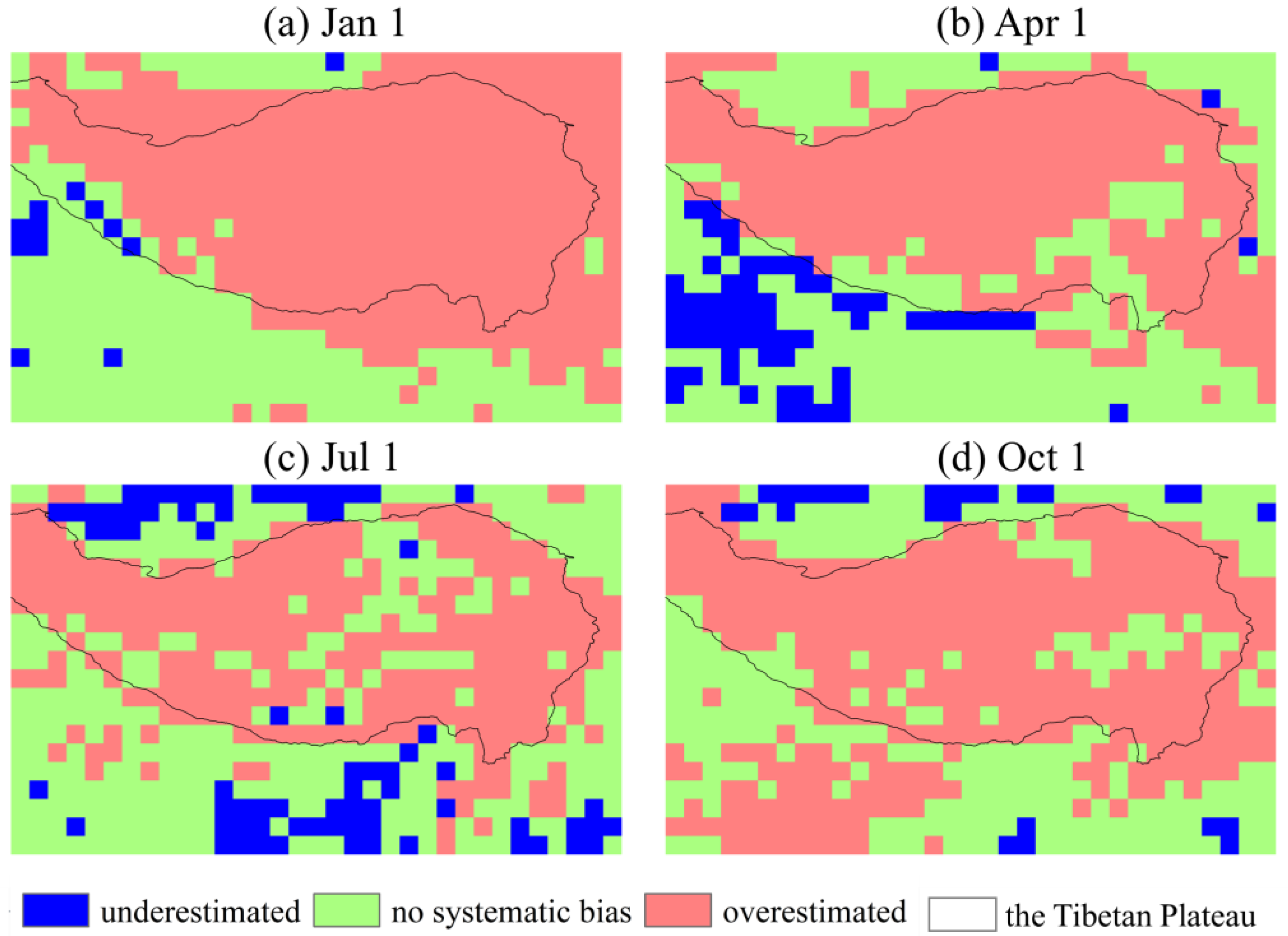
The evaluation process commenced by assessing precipitation forecast data for systematic errors and identifying their characteristics. For each of the 13 years from 2008 to 2020, cumulative precipitation over the subsequent 32 days was calculated using both forecast and observational data. If the forecasted value exceeded the measured value in more than 75% of cases (10 out of 13 pairs), the forecast for that date was classified as systematically overestimated. Conversely, if the forecasted value was less than the measured value in over 75% of cases, it was classified as systematically underestimated.
Corrections were subsequently applied based on the LS method to areas identified as systematically overestimated or underestimated. Correction factors representative of specific dates of the year were determined by summing 13 pairs of values (accumulated forecasted and observed precipitation over the next 32 days) for the same date across each year. Correction factors α t and corrected precipitation P y , t , i b c were calculated using the following equations:
α t =     y = 2008 2020 i = 1 L P y , t , i o b s     /   y = 2008 2020 i = 1 L P y , t , i f r c
P y , t , i b c =   α t   P y , t , i f r c
where y is the year from 2008 to 2020, t is the date of the year, and the others are the same as in Equations (1) and (2). The period from 2008 to 2020, during which the correction factors were derived from precipitation data, is designated as the calibration period. Subsequently, the 2021–2023 data served as the validation period for assessing the validity of these factors.
Finally, the efficacy of the precipitation bias correction was verified. Hydrological models in three basins were forced with three types of precipitation data: original forecasts, corrected forecasts, and observations. The resulting simulations were then compared against those driven by observed precipitation. This approach, rather than using measured streamflow as the benchmark, isolates the impact of precipitation errors by excluding uncertainties from other model inputs and the hydrological model itself. Total water volume is a crucial target for long-term hydrological forecasting. Systematic deviation in precipitation patterns across extensive regions may propagate inaccuracies in total water volume estimates. Our overarching aim is to mitigate systemic biases inherent in precipitation data and enhance the predictive precision of hydrological variables, particularly total water volume. Consequently, the relative error in total water volume emerged as the primary metric for evaluating the efficacy of the correction.

2.4. Hydrological Model

The hydrological model employed in this study is the Tsinghua Hydrological Model based on Representative Elementary Watershed (THREW) [63]. THREW integrates a set of equilibrium equations for mass, momentum, energy, and entropy, along with constitutive relationships governing various fluxes between representative units and sub-regions within these units. This model has demonstrated versatility across watersheds characterized by diverse climates and geological conditions, including applications in the Urumqi River basin [64], Han River basin [65], and Brahmaputra River basin [66].
In this study, THREW models were developed for the Upper Mekong basin, Upper Salween basin, and Brahmaputra basin. The data used for model construction, driving, and calibration were introduced earlier. The models operated on a daily scale. Calibration of the models utilized data from all hydrographic stations within the respective basins. The calibration process followed a sequential approach; parameters of the model in the upstream region were calibrated using data from the most upstream hydrological station (denoted as A). Subsequently, parameters in the region between stations A and the next downstream station (denoted as B) were calibrated using data from station B.
The calibration optimization target was the Nash–Sutcliffe Efficiency (NSE), given by:
N S E = 1 t = 1 n   Q t o b s Q t s i m 2 t = 1 n   Q t o b s Q o b s ¯ 2
where Q t o b s and Q t s i m are the daily streamflow for the observed and simulated time series, respectively. Q o b s ¯ is the average value of the observed streamflow.
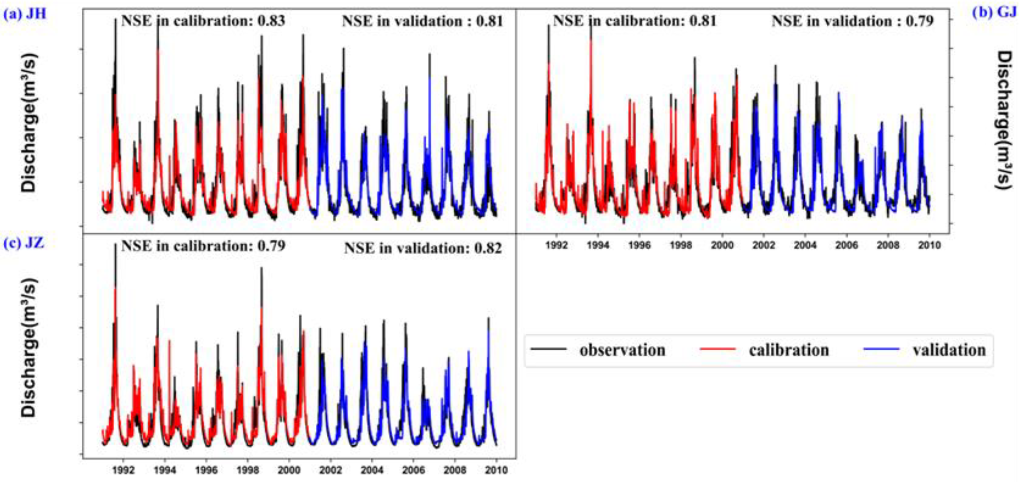
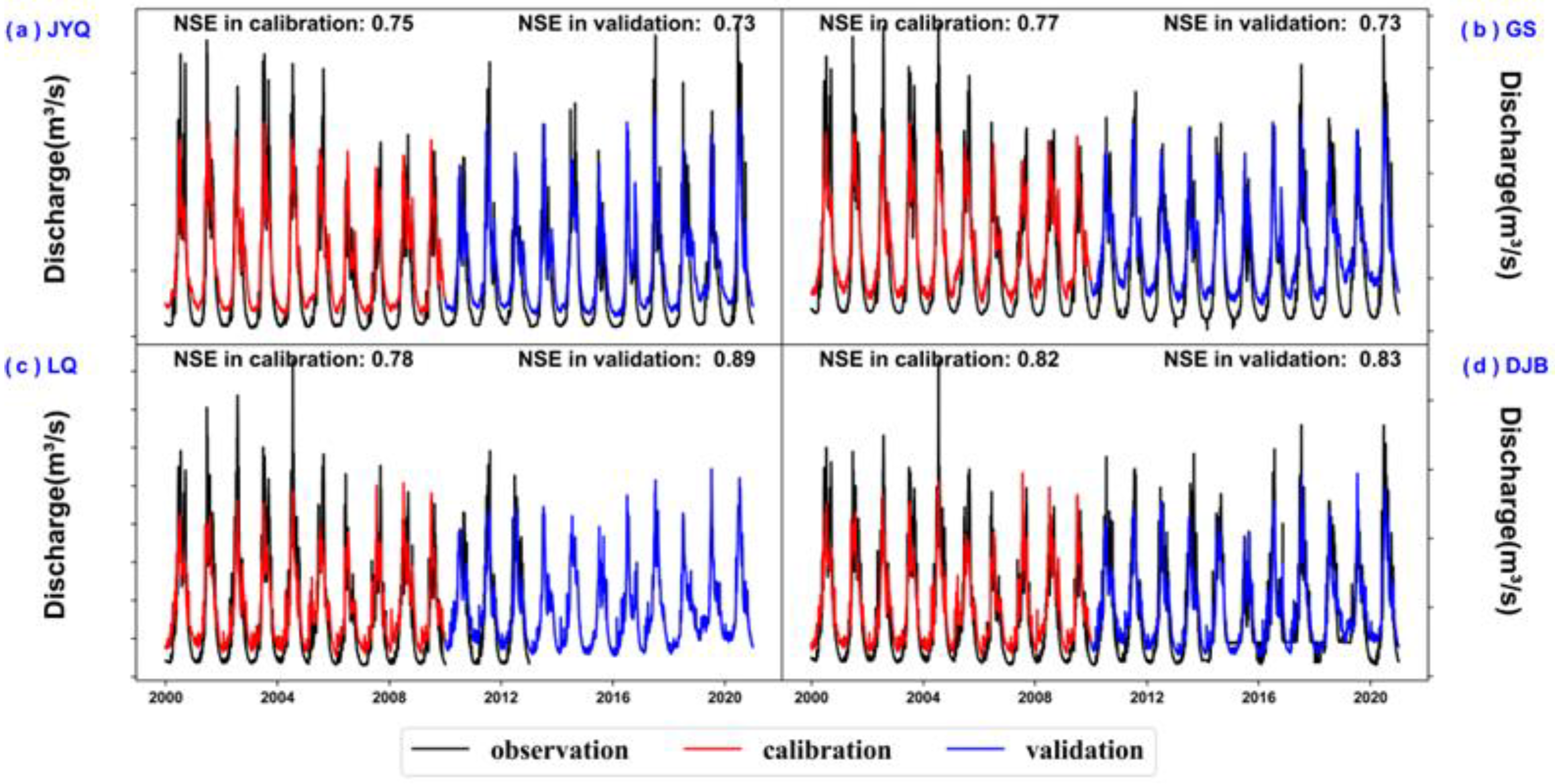
The performance of the model on a daily scale across three study basins evaluated at nine hydrological stations is presented in Table 1. The time series of the simulated and measured streamflow at the hydrological stations in the Upper Mekong and Salween River Basins Figures are illustrated in Figure A1 and Figure A2 in Appendix A. Detailed results for the Brahmaputra River Basin can be found in the previous study by Lyu et al. [67]. Notably, the hydrological models demonstrated excellent performance in all basins during both the calibration and validation periods, with Nash–Sutcliffe Efficiency (NSE) values exceeding 0.75, and more than half surpassing 0.8.

3. Results

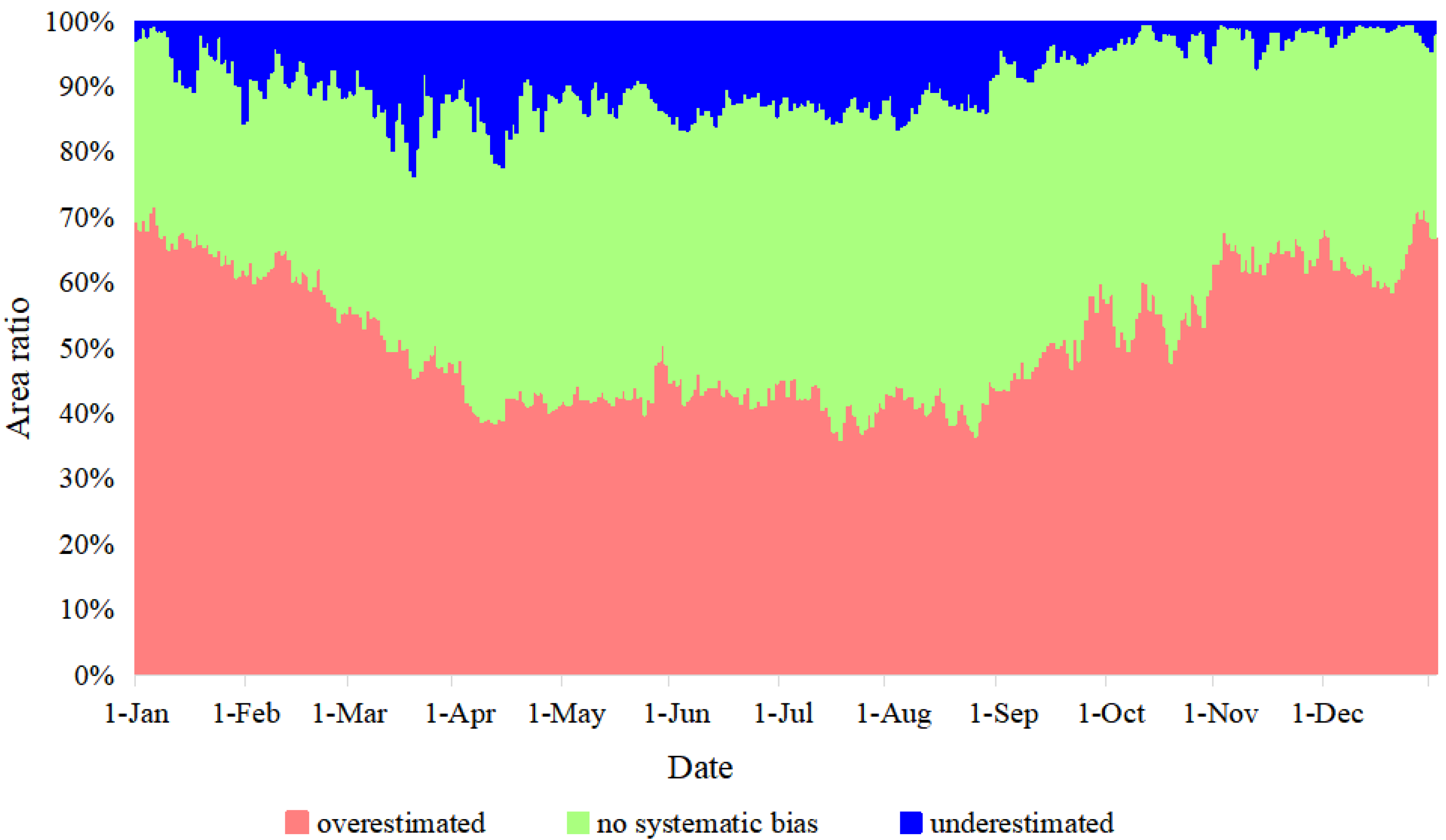
The evaluation of precipitation forecasts, as detailed in Section 2.3, yielded results illustrated in Figure 2, which are consistent across other dates. The daily area ratio, highlighting regions with systematic bias, is presented in Figure 3. Notably, the results indicate a prevalent overestimation of precipitation in most areas. Specifically, 40–70% of the study area experiences overestimation, while underestimation is limited to 0–20% of the region. The overestimation is more pronounced during the dry season, covering a larger geographical extent.
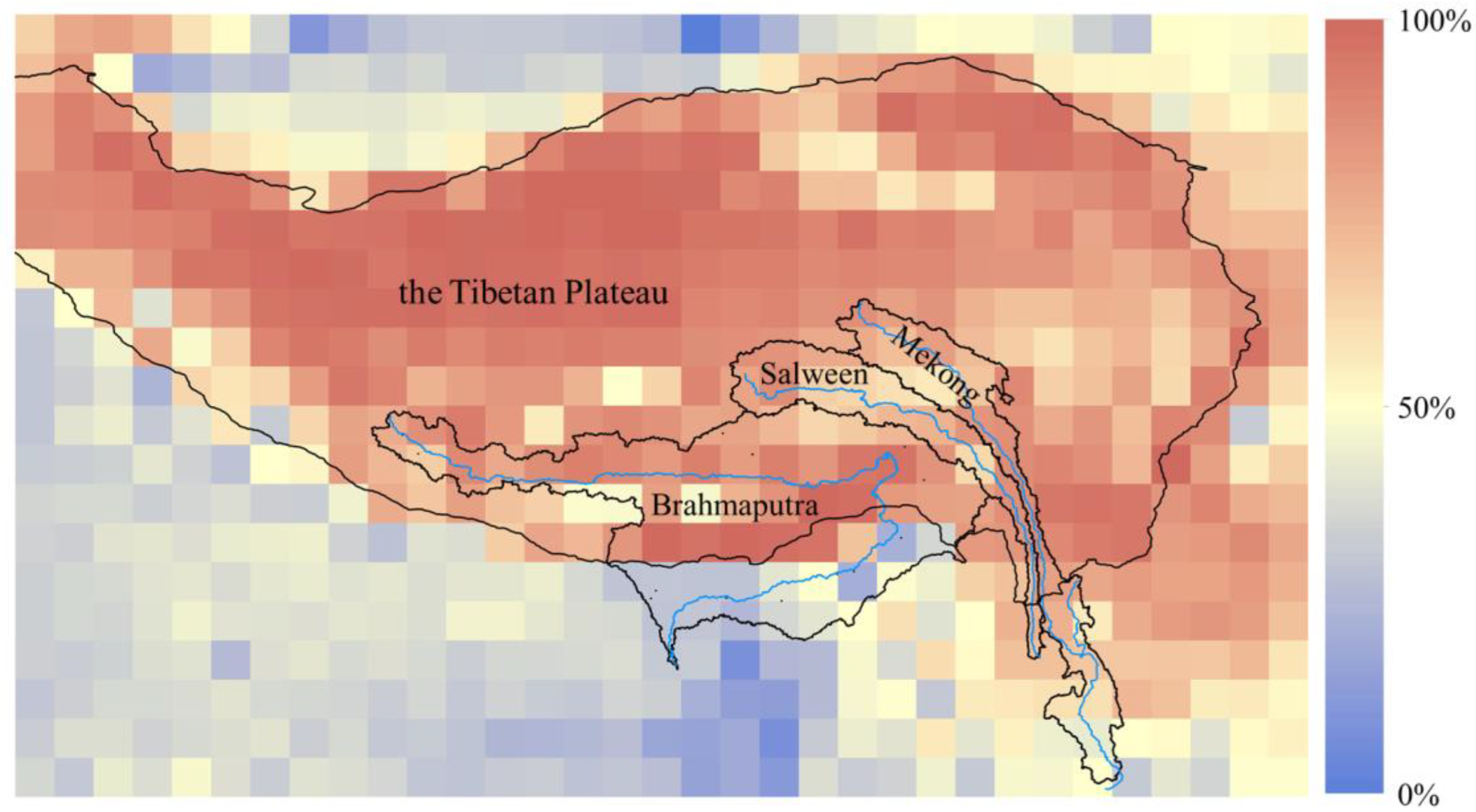
Spatially, the areas of overestimation closely correspond to the topography of the Tibetan Plateau, especially its high-altitude regions along the ridges with a significant altitudinal gradient. In contrast, the distribution of the underestimated area appears relatively random on a daily scale. An examination of the mean frequency of bias, illustrated in Figure 4, reveals that the underestimated areas are predominantly located in the estuary delta region of the Ganges and Brahmaputra, characterized by abundant precipitation to the south of the Tibetan Plateau, and the arid Tarim Basin to the north.
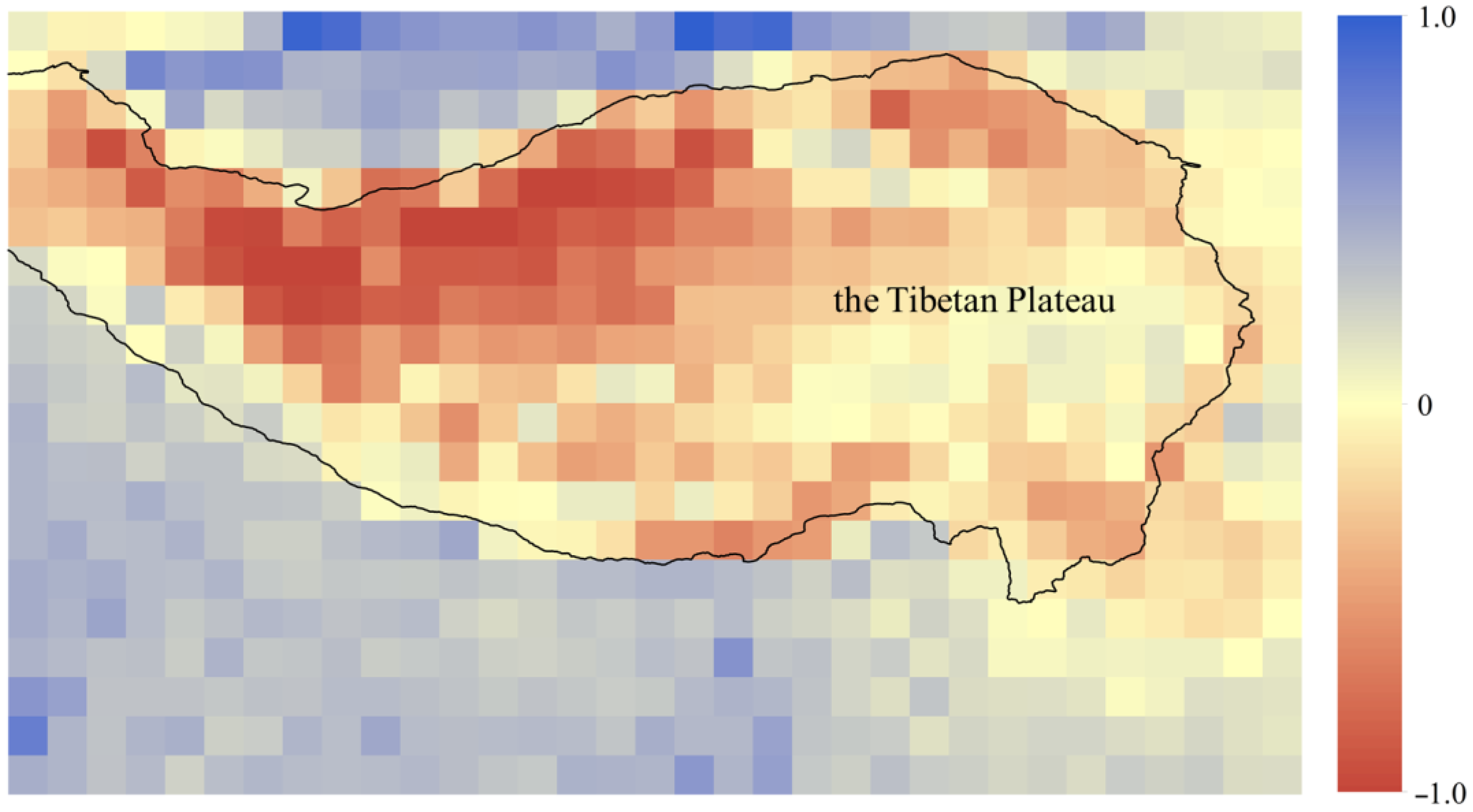
Applying the methodology detailed in Section 2.3, correction factors were calculated using ECMWF precipitation forecast data and GPM IMERG precipitation observation data. Figure 5 illustrates the spatial distribution of the base-10 logarithm of the mean correction factors. Logarithmic values, below zero, signify an average correction factor of less than one, indicating a prevalent overestimation of rainfall in the region. Conversely, positive logarithmic values denote underestimation. Notably, the logarithmic boundary line closely aligns with the topographical boundary of the Tibetan Plateau, which is consistent with previous frequency bias results. The correction factor, serving as a quantification of bias, provides further insight into the extent of overestimation, particularly in the northwestern part and along the ridgeline in the southern Brahmaputra basin within the Tibetan Plateau.
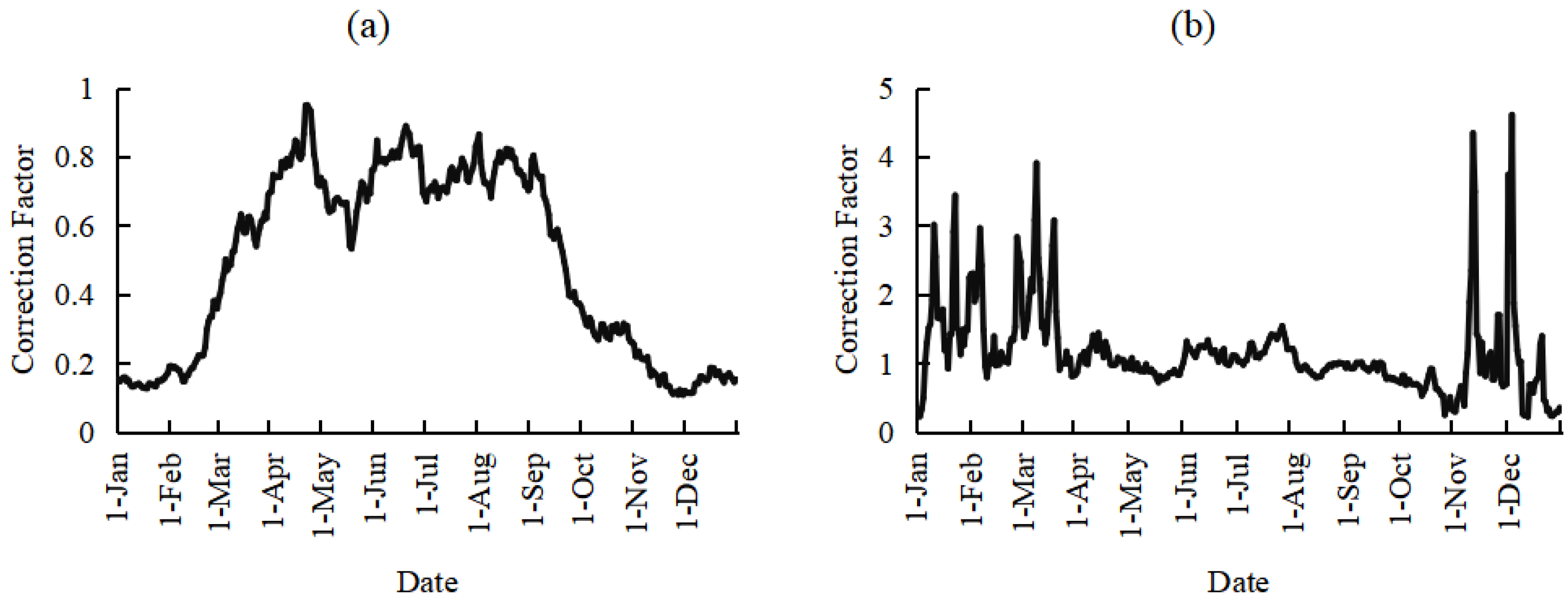
As exemplars, the time series of correction factors at the Nuxia and Bahadurabad hydrological stations in the Brahmaputra River basin are illustrated in Figure 6. In Nuxia, a region characterized by systematic overestimation of precipitation, the correction factor remains consistently below 1.0 throughout the year, with lower values observed during the dry season compared to the rainy season. This indicates a pronounced overestimation during the dry season, while the rainfall forecasts in the rainy season, although still overestimated, demonstrate relatively greater accuracy. Similar trends are observed in other regions where precipitation is overestimated. Conversely, Bahadurabad, located in an area where precipitation is underestimated, exhibits varying correction factors. During the rainy season, the correction factors fluctuate around 1.0, suggesting relatively accurate precipitation forecasts. However, in the dry season, precipitation is consistently underestimated. Comparable trends are noted in other regions where precipitation is underestimated.
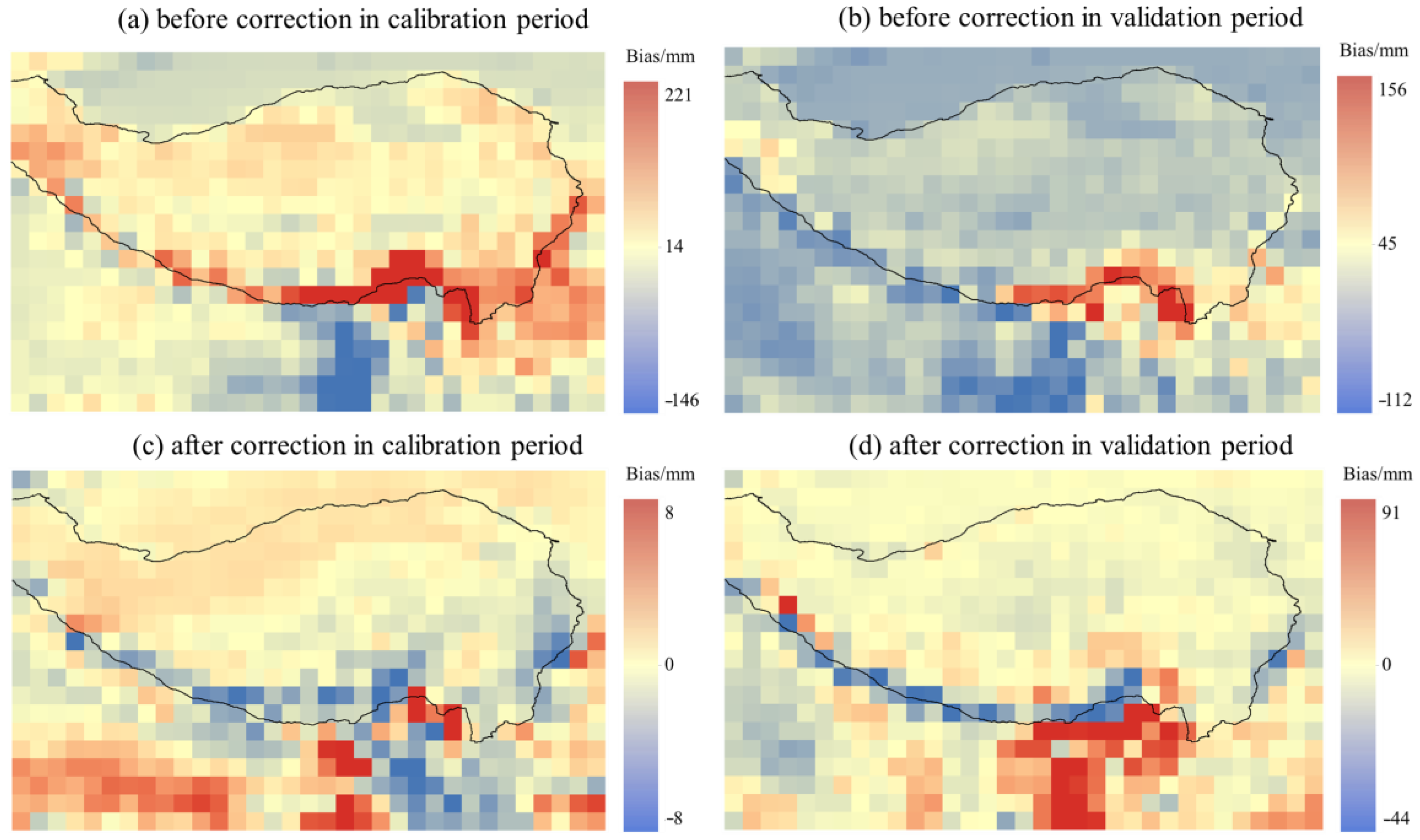
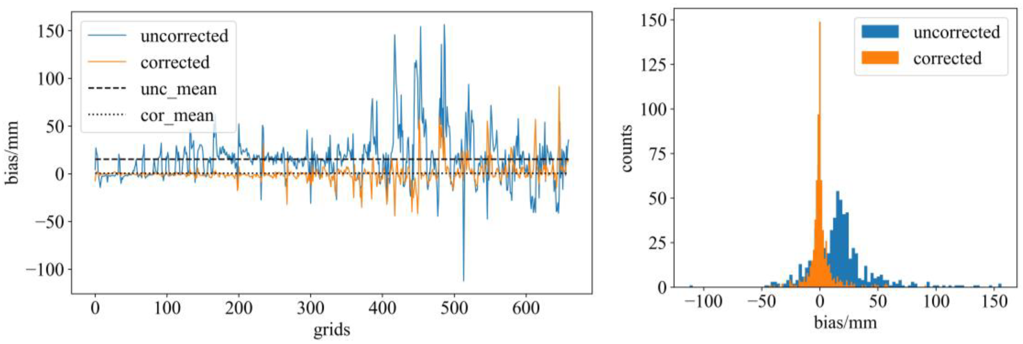
The spatial distribution of the mean bias of the 32-day cumulative precipitation both before and after correction, during the calibration period (2008–2020) and the validation period (2021–2023), is illustrated in Figure 7. Additionally, as an important metric, the mean bias on each grid before and after correction during the validation period is presented in Figure 8. The pattern of mean bias before correction in the calibration period is consistent with the pattern of mean frequency of overestimation, exhibiting a mean of 15 mm, a maximum of 221 mm and a minimum of −146 mm. After correction, the mean bias is reduced to 0, and the range of variation is significantly narrowed. Such a low bias is anticipated during the calibration period. During the validation period, the pattern of the mean bias before correction remains consistent with that during the calibration period, with a mean of 15 mm, a maximum of 156 mm and a minimum of −112 mm. After correction, the mean bias is reduced to 0.6 mm, and the range of variation is also confined to between 91 mm and −44 mm. The standard deviation decreases from 26.2 mm to 10.8 mm. Most grid points exhibit a reduction in bias, although some grids show a reversal in bias. Prior to bias correction, grids located along the southern border of the Tibetan Plateau display positive (overestimated) biases; however, after correction, these grids exhibit negative biases. Conversely, the delta areas of the Ganges and Brahmaputra estuaries, which initially demonstrated negative biases, showed positive biases after correction. Nevertheless, even in these regions, the absolute value of the reversed bias is generally smaller than the original bias.
Overall, the precipitation bias over the whole study area is reduced after the correction.
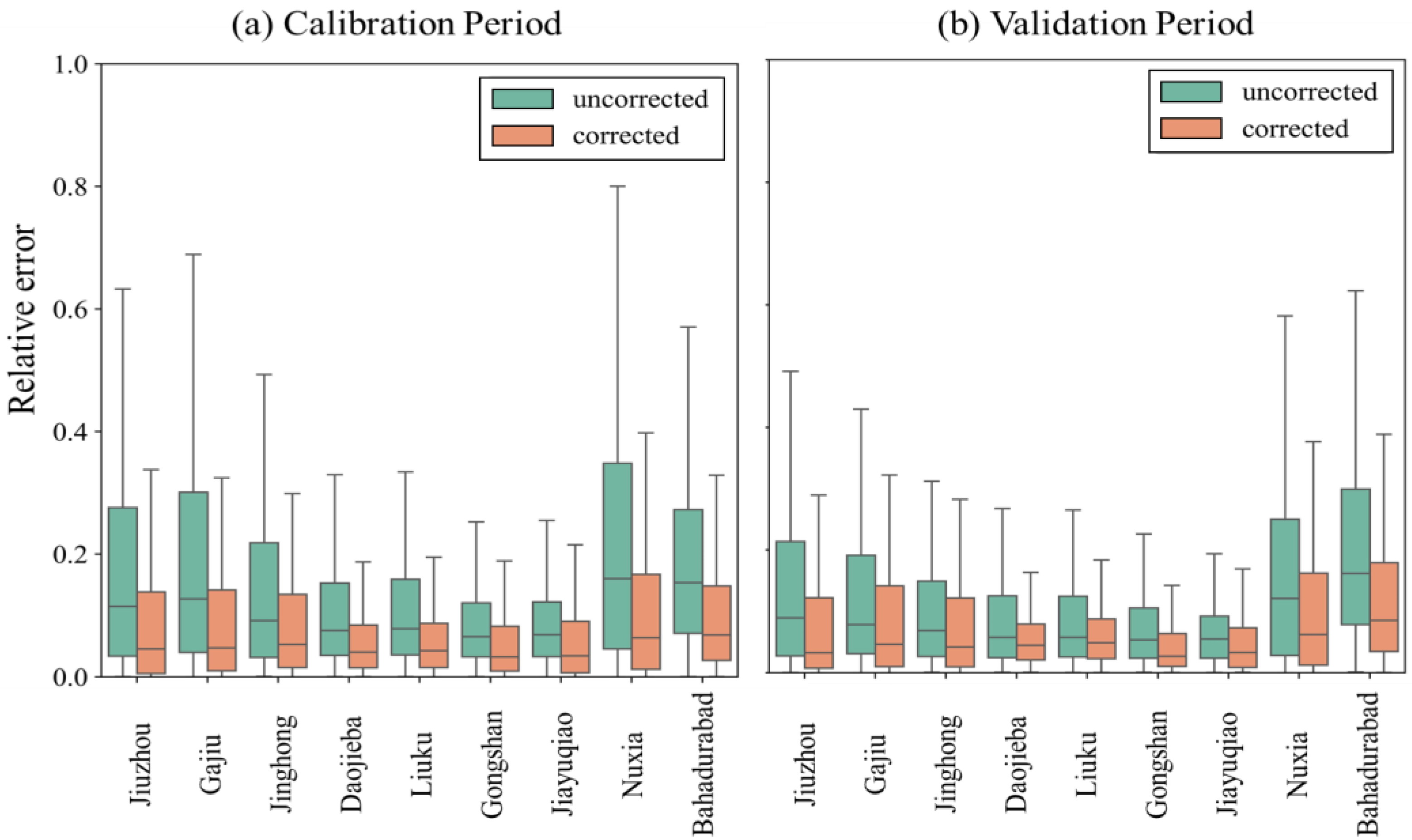
In an effort to isolate the effects of errors in other input data and the hydrological model itself, the results of the hydrological model driven by corrected forecasted precipitation were compared with those driven by measured precipitation, rather than measured streamflow. Utilizing 1398 precipitation forecasts from ECMWF, the original precipitation forecast data, corrected precipitation forecast data, and measured precipitation data were separately employed to drive the hydrological model. Subsequently, the total water volume over the next 32 days was calculated, and the relative error was determined. The results are presented in Figure 9 and Table 2.
The mean relative error before and after correction in the calibration period and the validation period is detailed in columns 3, 4 and 6, 7 of Table 2. A comparison of the relative errors in total water volume before and after bias correction demonstrates the efficacy of the correction applied to the original precipitation forecasts, particularly in the Brahmaputra basin, where the correction effect is notably significant. For stations such as Nuxia and Bahadurabad, the relative errors during the calibration period decreased from 25.32% and 20.37% to 9.58% and 8.36%, respectively. This reduction in relative error is consistent across all other stations during both calibration and validation periods, with the relative error nearly halved after correction.
The analysis evaluated the effectiveness of various corrections made during the calibration and validation periods by assessing how many of these corrections led to improvements in hydrological forecasting, particularly in terms of reducing relative error. Columns 5 and 8 in Table 2 illustrates the improvement frequency (IF). Remarkably, the correction method proved effective, enhancing the accuracy of hydrological forecasts in at least 70% of all forecasts across all stations during the calibration period, with this value exceeding 65% in the validation period. Notably, at the two stations located in the Brahmaputra River basin, the improvement frequency reached impressive levels of 95% and 89% during the calibration and validation period, respectively.
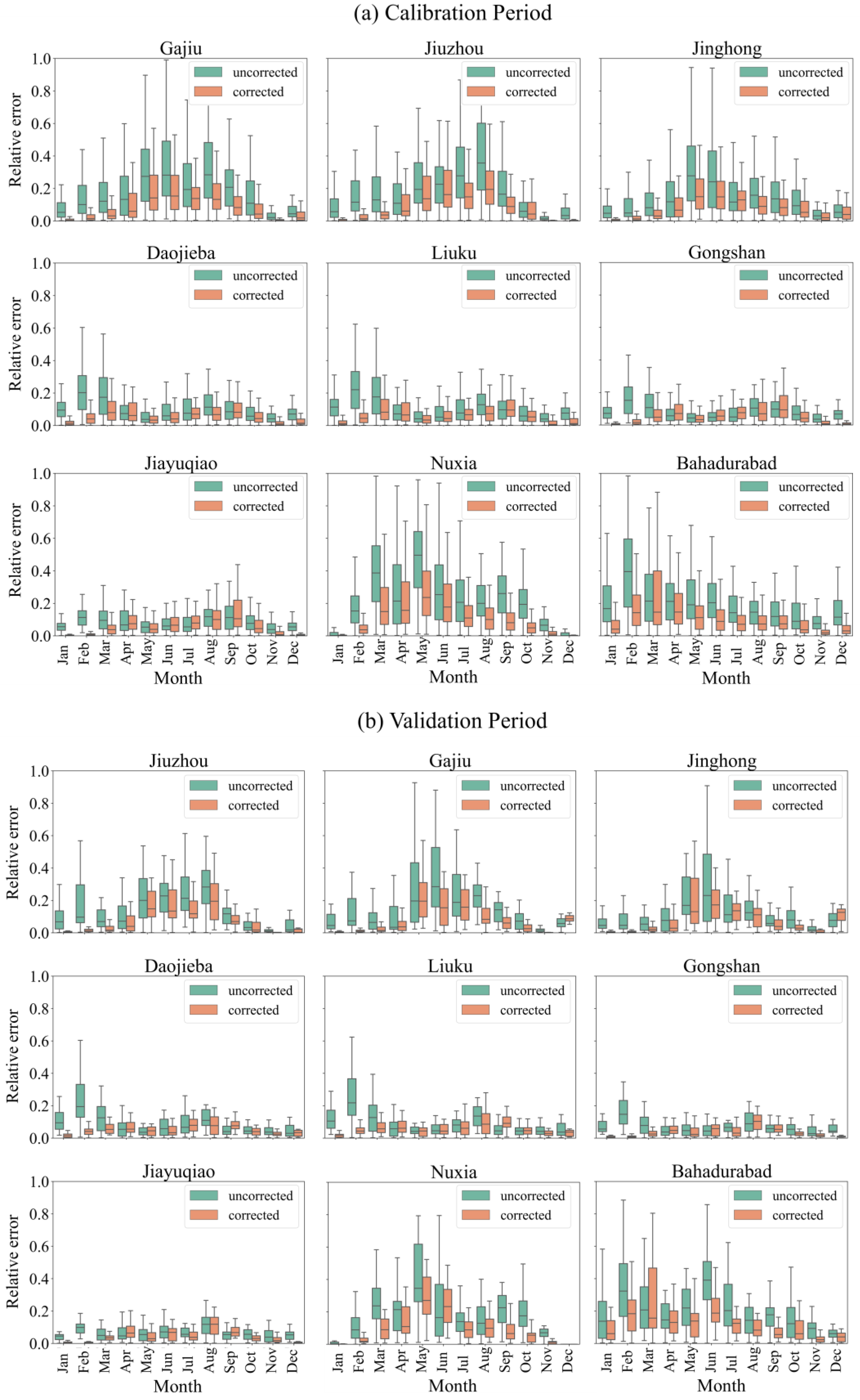
Considering that precipitation characteristics, including total amount and intensity, typically exhibit significant seasonal variations, and that Figure 2 and Figure 6 reveal corresponding temporal patterns in the forecast bias and its correction factors, we aggregated the relative error of total water volume at hydrological stations across the three study basins before and after the correction of precipitation bias during the calibration and validation periods on a monthly scale. This approach allows us to assess the method’s performance across different seasons, with the results presented in Figure 10.
In the Upper Mekong River Basin, the relative error for the three stations was predominantly concentrated during the flood season from May to August, exhibiting relatively high averages and variability. Following precipitation correction, the relative error decreased significantly across all months, particularly in the cold season, where the average relative error nearly approached zero. The four stations in the Salween River Basin exhibited a relatively smaller relative error compared to the other two basins both before and after correction. The original relative error was primarily noted in February and March, and after precipitation correction, the average relative error for most months fell below 10%. In the Brahmaputra River Basin, the relative error was mainly observed in the pre-flood months from February to May, and precipitation correction also contributed to a reduction in relative error in this basin. At Bahadurabad station, the variability range in March increased slightly after correction, although the average value still declined. During the validation period, the overall trend mirrored that of the calibration period, with both the average and range of relative error decreasing in most months after correction. Nonetheless, certain stations exhibited anomalies in specific months, for instance, Gongshan Station experienced a slight increase in both the mean and range of relative error in September after precipitation correction, although this increase was not significant.

4. Discussion

4.1. Impact of the Selection of Correction Factors

The results demonstrate the effectiveness of the correction method and correction factor series in enhancing the accuracy of medium- and long-term hydrological forecasting, as evidenced by improvements in both the extent of error reduction and the frequency of successful corrections.
However, it is noteworthy that even during the calibration period, approximately 15–30% of cases in the upper Mekong and upper Salween basins exhibited a greater relative error in hydrological forecasts after precipitation correction, compared to less than 5% in the Brahmaputra basin. This discrepancy may arise from varying degrees of systematic bias in precipitation forecasts across the three basins. Figure 4 and Figure 5 reveal that, particularly in the upper Brahmaputra region within the Tibetan Plateau, along the ridgelines, the frequency and magnitude of bias are more pronounced than in the upper Mekong and upper Salween basins. The upper Brahmaputra exhibited an average bias frequency of 86%, and an average logarithm of the correction factor of −0.35, while the corresponding values in the upper Mekong and upper Salween basins were 76%, −0.17 and 79%, −0.23, respectively. Notably, along the ridgelines in the upper Brahmaputra, the average bias frequency exceeded 95%, and the average logarithm of the correction factor was lower than −0.5. Due to the more stable and substantial systematic errors in the Brahmaputra basin, determining a stable and effective correction factor is relatively easier.
In the other two basins, while systematic bias is present, it exhibits a more random pattern. Applying a uniform correction factor to each forecast may lead to over-correction of precipitation in certain instances, resulting in reverse errors. For instance, in areas that are consistently overestimated, there is a risk of excessively reducing precipitation after correction. This study evaluated the systematic deviation in forecast data over the past 15 years in these basins. The question arose: Can a correction factor be determined based on the frequency of systematic bias, thereby preventing over-correction of precipitation and ensuring improved accuracy in hydrological forecasts across a broader spectrum of cases?
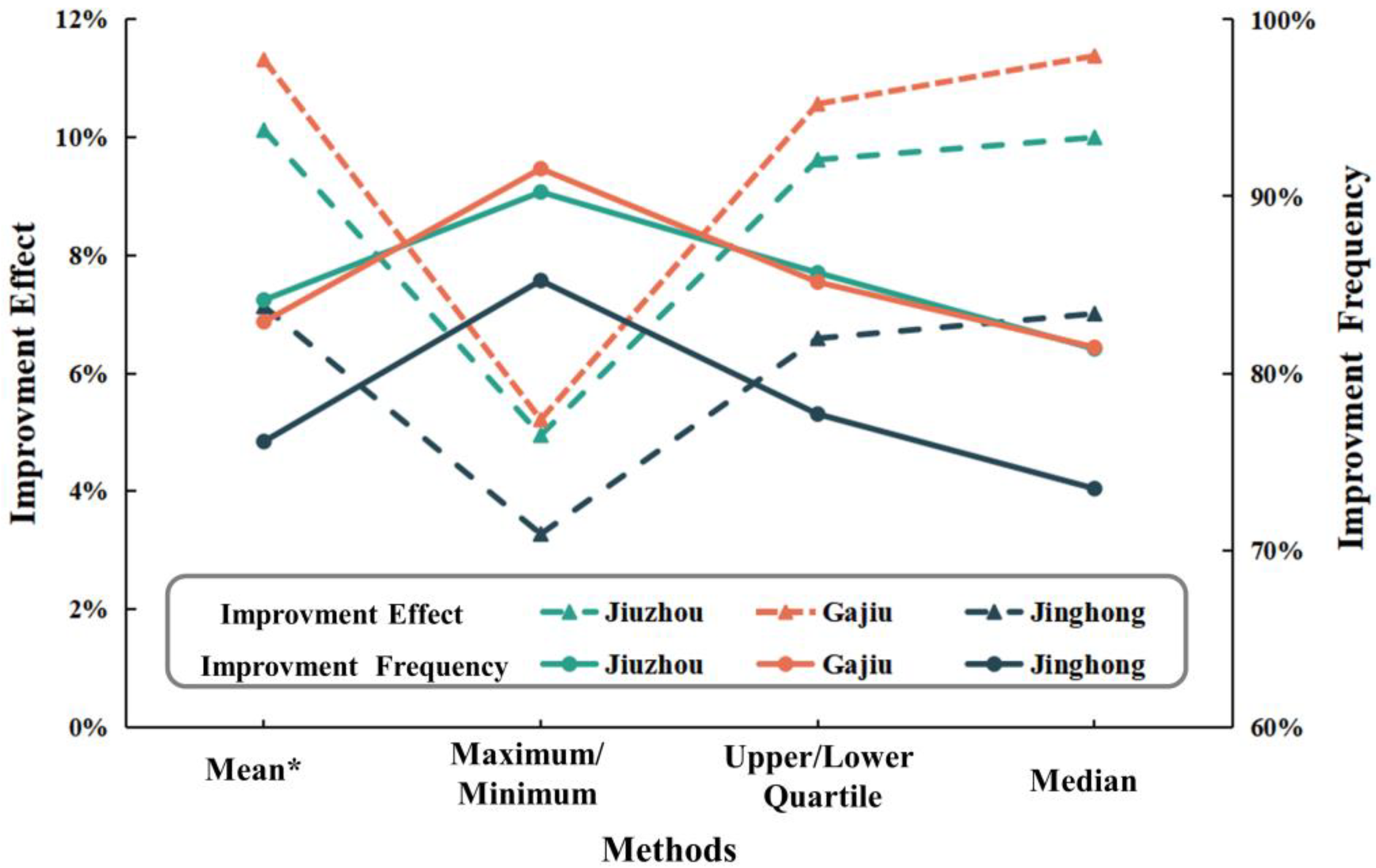
In the preceding section, 13 pairs of cumulative forecasted and observed precipitation for each year, spanning from 2008 to 2020 on the same date, were computed to establish bias frequencies. Subsequently, 13 correction factors were derived from these pairs using Equation (1). In cases of overestimation, any correction factor less than 1 effectively corrects the forecasted data. Consequently, for systematically overestimated areas (grids), the correction factors were filtered to identify those less than 1.0, which were then sorted. The maximum value, upper quartile, and median of these selected correction factors were employed individually as correction factors. Similarly, for systematically underestimated areas (grids), the correction factors greater than 1.0 were filtered, sorted, and the minimum value, lower quartile, and median were utilized as correction coefficients, respectively. These correction factors were applied separately to correct precipitation and subsequently drove the hydrological model in the upper Mekong basin as an example. The results are shown in Figure 11.
The results indicate that the frequency of improvement increases when the maximum or minimum correction factor is applied. This phenomenon can be attributed to the correction of precipitation bias in most instances without overcorrection. However, concurrently, the improvement effect decreases as the precipitation bias is only marginally corrected through this conservative approach. In comparison to the maximum (or minimum) value, when the upper (or lower) quartile and median are applied, the improvement frequency decreases, but the improvement effect increases. This suggests that when employing the linear scaling method in regions where the linear relationship between predictions and observations is weak, the improvement effect and frequency can become contradictory optimization objectives when a fixed correction factor is applied. This phenomenon arises from the differing expected correction factors that correspond to different cases. In practical hydrological forecasting, the selection of appropriate correction factors should be guided by a balanced consideration of the desired objectives, whether they prioritize effectiveness or probability.

4.2. Limitations and Future Outlook

While our study has contributed to uncovering the spatial and temporal distribution of biases in the ECMWF extended forecast of precipitation for the study region and improving long-term streamflow forecasting accuracy by correcting the raw precipitation forecast, it is essential to acknowledge certain limitations that should be considered in future research endeavors.
As mentioned in the Introduction section, numerous bias correction and post-processing methods have been proposed [17,18,19,20,21,22,23,24,25,26,27,28,29], each demonstrating varying performance depending on the modeling chain and the study area. Given that the straightforward bias correction method, the LS method, proved effective in reducing precipitation biases and enhancing hydrological forecasts in this study, no additional bias correction methods were adopted, nor were comparative studies conducted. This work provides a foundation for future investigations into comparative studies.
As a pioneering study, this study is based on the ECMWF’s control forecasts and the IMERG Final Run dataset, conducted at a 1° spatial resolution with a 32-day lead time, utilizing the Linear Scaling method for bias correction. Further research is expected to explore several areas that could provide a more comprehensive understanding and further improve streamflow forecasting accuracy in the study area. These areas include the use of all ensemble members, higher-precision observational data, evaluations across more spatial and temporal scales, and comparative analyses of various post-processing methods.

5. Conclusions

This study focuses on evaluating and correcting the ECMWF long-term precipitation forecasts over the confluence of the Asian monsoons and westerlies, emphasizing the derivation of time series correction factors for hydrological forecasting. The analysis revealed a significant systematic bias in the ECMWF Set VI-ENS forecasted precipitation data over the study area. Specifically, the ECMWF Set VI-ENS forecasted precipitation data exhibited a notable systematic bias over the confluence area of the Asian monsoons and westerlies. Approximately half of the region, particularly the entire Tibetan Plateau, experienced overestimated precipitation, with higher relative errors observed during dry seasons compared to wet seasons. Additionally, the application of the linear scaling method for bias correction on the original forecasted precipitation data proved effective. Notably, the Brahmaputra River basin demonstrated substantial correction effects, leading to a significant reduction in the relative error of total water in hydrological forecasts—from 25% to 10% during the calibration period and from 20% to 9% during the validation period. This correction proved effective in over 90% and 85% of hydrological forecasts at Nuxia for the two periods, respectively. Across all hydrographic stations in the three study basins, the ratio exceeded 70% and 65%.
Nevertheless, in specific regions where the linear relationship between forecasted and actual values was weak, the effectiveness and frequency of bias correction using linear scaling methods showed contradictions, highlighting the need for careful consideration and adjustment of correction factors based on specific objectives in practical hydrological forecasting.
These findings underscore the presence of significant systematic bias in long-term precipitation forecasts, particularly in areas with complex physiogeographic conditions. Such biases should be taken into account when utilizing ECMWF forecast data. As ground-based precipitation measurement infrastructure improves, future evaluations and corrections are anticipated to become more accurate and reliable.

Author Contributions

Conceptualization, resources, writing—review: M.T., F.T., K.Z. and H.L.; methodology, visualization: M.T.; software, data curation: M.T. and K.Z.; investigation, validation: M.T., K.Z. and H.L.; supervision, funding acquisition: F.T. All authors have read and agreed to the published version of the manuscript.

Funding

This research was funded by the National Key Research and Development Program of China under grant numbers 2024YFC3013304 and 2022YFC3002900.

Data Availability Statement

The original contributions presented in this study are included in the article. For more information, please contact the corresponding author.

Acknowledgments

The authors acknowledge the contributions of these data source including ECMWF, GPM, MERIT and NOAA Climate Data Record (CDR).

Conflicts of Interest

The authors declare no conflicts of interest.

Appendix A

The time series of the simulated and measured streamflow during the calibration and validation period at hydrological stations in the Upper Mekong and Salween River Basin are showed in Figure A1 and Figure A2, respectively. Due to confidentiality reasons, the vertical axis has been concealed.
Figure A1. The time series of the simulated and measured streamflow during the calibration and validation period at hydrological stations in the Upper Mekong River Basin.
Hydrology 12 00218 g0a1
Figure A2. The time series of the simulated and measured streamflow during the calibration and validation period at hydrological stations in the Salween River Basin.
Hydrology 12 00218 g0a2

References

  1. Ng, K.W.; Huang, Y.F.; Koo, C.H.; Chong, K.L.; El-Shafie, A.; Ahmed, A.N. A review of hybrid deep learning applications for streamflow forecasting. J. Hydrol. 2023, 625, 130141. [Google Scholar] [CrossRef]
  2. Cheng, M.; Fang, F.; Kinouchi, T.; Navon, I.M.; Pain, C.C. Long lead-time daily and monthly streamflow forecasting using machine learning methods. J. Hydrol. 2020, 590, 125376. [Google Scholar] [CrossRef]
  3. Sun, A.Y.; Wang, D.; Xu, X. Monthly streamflow forecasting using Gaussian process regression. J. Hydrol. 2014, 511, 72–81. [Google Scholar] [CrossRef]
  4. Ni, L.; Wang, D.; Singh, V.P.; Wu, J.; Wang, Y.; Tao, Y.; Zhang, J. Streamflow and rainfall forecasting by two long short-term memory-based models. J. Hydrol. 2019, 583, 124296. [Google Scholar] [CrossRef]
  5. Gomez, M.; Sharma, S.; Reed, S.; Mejia, A. Skill of ensemble flood inundation forecasts at short-to medium-range timescales. J. Hydrol. 2019, 568, 207–220. [Google Scholar] [CrossRef]
  6. Sharma, S.; Raj Ghimire, G.; Siddique, R. Machine learning for postprocessing ensemble streamflow forecasts. J. Hydroinform. 2023, 25, 126–139. [Google Scholar] [CrossRef]
  7. Yang, C.; Yuan, H.; Su, X. Bias correction of ensemble precipitation forecasts in the improvement of summer streamflow prediction skill. J. Hydrol. 2020, 588, 124955. [Google Scholar] [CrossRef]
  8. Su, X.; Yuan, H.; Zhu, Y.; Luo, Y.; Wang, Y. Evaluation of TIGGE ensemble predictions of Northern Hemisphere summer precipitation during 2008–2012. J. Geophys. Res. Atmos. 2014, 119, 7292–7310. [Google Scholar] [CrossRef]
  9. Lavers, D.A.; Harrigan, S.; Prudhomme, C. Precipitation Biases in the ECMWF Integrated Forecasting System. J. Hydrometeor. 2021, 22, 1187–1198. [Google Scholar] [CrossRef]
  10. Li, W.; Hu, S.; Hsu, P.C.; Guo, W.; Wei, J. Systematic bias of Tibetan Plateau snow cover in subseasonal-to-seasonal models. Cryosphere 2020, 14, 3565–3579. [Google Scholar] [CrossRef]
  11. Yuan, W.H.; Hu, X.L.; Li, Y.S. Evaluation of the hourly rainfall in the ECMWF forecasting over southwestern China. Meteor. Appl. 2020, 27, e1936. [Google Scholar] [CrossRef]
  12. Xie, Y.; Yuan, W.; Hu, X. Evaluation of hourly forecasts of the European Centre for Medium-Range Weather Forecasts over the southeastern extension of the Tibetan Plateau. Int. J. Climatol. 2022, 42, 5232–5241. [Google Scholar] [CrossRef]
  13. Liu, C.; Sun, J.; Yang, X.; Jin, S.; Fu, S. Evaluation of ECMWF precipitation predictions in China during 2015–18. Weather Forecast. 2021, 36, 1043–1060. [Google Scholar] [CrossRef]
  14. Verkade, J.S.; Brown, J.D.; Reggiani, P.; Weerts, A.H. Post-processing ECMWF precipitation and temperature ensemble reforecasts for operational hydrologic forecasting at various spatial scales. J. Hydrol. 2013, 501, 73–91. [Google Scholar] [CrossRef]
  15. Pappenberger, F.; Cloke, H.L.; Balsamo, G.; Ngo-Duc, T.; Oki, T. Global runoff routing with the hydrological component of the ECMWF NWP system. Int. J. Climatol. 2010, 30, 2155–2174. [Google Scholar] [CrossRef]
  16. Balsamo, G.; Viterbo, P.; Beljaars, A.; den Hurk, B.V.; Hirchi, M.; Betts, A.; Scipal, K. A revised hydrology for the ECMWF model: Verification from field site to terrestrial water storage and impact in the integrated forecast system. J. Hydrometeorol. 2008, 10, 623–643. [Google Scholar] [CrossRef]
  17. Gneiting, T.; Raftery, A.; Westveld, A.; Goldman, T. Calibrated probabilistic forecasting using ensemble model output statistics and minimum CRPS estimation. Mon. Weather Rev. 2005, 133, 1098–1118. [Google Scholar] [CrossRef]
  18. Hagedorn, R.; Hamill, T.; Whitaker, J. Probabilistic forecast calibration using ECMWF and GFS ensemble reforecasts. Part I: Two-meter temperatures. Mon. Weather Rev. 2008, 136, 2608–2619. [Google Scholar] [CrossRef]
  19. Roulin, E.; Vannitsem, S. Postprocessing of Ensemble Precipitation Predictions with Extended Logistic Regression Based on Hindcasts. Mon. Weather Rev. 2012, 140, 874–888. [Google Scholar] [CrossRef]
  20. Wilks, D.S. Extending logistic regression to provide full-probability-distribution MOS forecasts. Meteorol. Appl. 2009, 16, 361–368. [Google Scholar] [CrossRef]
  21. Block, P.J.; Souza-Filho, F.A.; Sun, L.; Kwon, H.H. A Stream-flow Forecasting Framework using Multiple Climate and Hydrological Models. J. Am. Water Resour. Assoc. 2009, 45, 828–843. [Google Scholar] [CrossRef]
  22. Déqué, M.; Rowell, D.P.; Lüthi, D.; Giorgi, F.; Christensen, J.H.; Rockel, B.; Jacob, D.; Kjellström, E.; de Castro, M.; Van Den Hurk, B. An intercomparison of regional climate simulations for Europe: Assessing uncertainties in model projections. Clim. Change 2007, 81, 53–70. [Google Scholar] [CrossRef]
  23. Kim, D.I.; Kwon, H.H.; Han, D. Bias correction of daily precipitation over South Korea from the long-term reanalysis using a composite Gamma-Pareto distribution approach. Hydrol. Res. 2019, 50, 1138–1161. [Google Scholar] [CrossRef]
  24. Sloughter, J.M.L.; Raftery, A.E.; Gneiting, T.; Fraley, C. Probabilistic quantitative precipitation forecasting using Bayesian Model Averaging. Mon. Weather Rev. 2007, 135, 3209–3220. [Google Scholar] [CrossRef]
  25. Hamill, T.M.; Hagedorn, R.; Whitaker, J.S. Probabilistic Forecast Calibration Using ECMWF and GFS Ensemble Reforecasts. Part II: Precipitation. Mon. Weather Rev. 2008, 136, 2620–2632. [Google Scholar] [CrossRef]
  26. Ma, Y.; Yang, Y.; Han, Z.; Tang, G.; Maguire, L.; Chu, Z.; Hong, Y. Comprehensive evaluation of Ensemble Multi-Satellite Precipitation Dataset using the Dynamic Bayesian Model Averaging scheme over the Tibetan plateau. J. Hydrol. 2018, 556, 634–644. [Google Scholar] [CrossRef]
  27. Yuan, H.; Gao, X.; Mullen, S.L.; Sorooshian, S.; Du, J.; Juang, H.-M.H. Calibration of probabilistic quantitative precipitation forecasts with an artificial neural network. Weather Forecast. 2007, 22, 1287–1303. [Google Scholar] [CrossRef]
  28. Wilks, D.S.; Hamill, T.M. Comparison of ensemble-MOS methods using GFS reforecasts. Mon. Weather Rev. 2007, 135, 2379–2390. [Google Scholar] [CrossRef]
  29. Mendez, M.; Maathuis, B.; Hein-Griggs, D.; Alvarado-Gamboa, L.-F. Performance Evaluation of Bias Correction Methods for Climate Change Monthly Precipitation Projections over Costa Rica. Water 2020, 12, 482. [Google Scholar] [CrossRef]
  30. Crochemore, L.; Ramos, M.H.; Pappenberger, F. Bias correcting precipitation forecasts to improve the skill of seasonal streamflow forecasts. Hydrol. Earth Syst. Sci. 2016, 20, 3601–3618. [Google Scholar] [CrossRef]
  31. Wang, P.; Clemens, S.; Beaufort, L.; Braconnot, P.; Ganssen, G.; Jian, Z.; Kershaw, P.; Sarnthein, M. Evolution and variability of the Asian monsoon system: State of the art and outstanding issues. Quat. Sci. Rev. 2005, 24, 595–629. [Google Scholar] [CrossRef]
  32. Tada, R.; Zheng, H.; Clift, P.D. Evolution and variability of the Asian monsoon and its potential linkage with uplift of the Himalaya and Tibetan Plateau. Prog. Earth Planet. Sci. 2016, 3, 4. [Google Scholar] [CrossRef]
  33. Ma, Q.; You, Q.; Ma, Y.; Cao, Y.; Zhang, J.; Niu, M.; Zhang, Y. Changes in cloud amount over the Tibetan Plateau and impacts of large-scale circulation. Atmos. Res. 2021, 249, 105332. [Google Scholar] [CrossRef]
  34. Lu, H.; Zheng, D.; Yang, K.; Yang, F. Last-decade progress in understanding and modeling the land surface processes on the Tibetan Plateau. Hydrol. Earth Syst. Sci. 2020, 24, 5745–5758. [Google Scholar] [CrossRef]
  35. Zhang, F.; Thapa, S.; Immerzeel, W.; Zhang, H.; Lutz, A. Water availability on the Third Pole: A review. Water Secur. 2019, 7, 100033. [Google Scholar] [CrossRef]
  36. Li, S.F.; Valdes, P.J.; Farnsworth, A.; Davies-Barnard, T.; Su, T.; Lunt, D.J.; Spicer, R.A.; Liu, J.; Deng, W.Y.D.; Huang, J.; et al. Orographic evolution of northern Tibet shaped vegetation and plant diversity in eastern Asia. Sci. Adv. 2021, 7, eabc7741. [Google Scholar] [CrossRef]
  37. Guo, D.; Wang, H. The significant climate warming in the northern Tibetan Plateau and its possible causes. Int. J. Climatol. 2012, 32, 1775–1781. [Google Scholar] [CrossRef]
  38. Kuang, X.; Jiao, J.J. Review on climate change on the Tibetan Plateau during the last half century. J. Geophys. Res. Atmos. 2016, 121, 3979–4007. [Google Scholar] [CrossRef]
  39. American Meteorological Society. Long-Term Hydrological Forecast. Glossary of Meteorology. 2025. Available online: https://glossary.ametsoc.org/wiki/Long-term_hydrological_forecast (accessed on 10 May 2025).
  40. Li, D.; Yang, K.; Tang, W.; Li, X.; Zhou, X.; Guo, D. Characterizing precipitation in high altitudes of the western Tibetan plateau with a focus on major glacier areas. Int. J. Climatol. 2020, 40, 5114–5127. [Google Scholar] [CrossRef]
  41. Zheng, H.; Yang, Q.; Cao, S.; Clift, P.D.; He, M.; Kano, A.; Sakuma, A.; Xu, H.; Tada, R.; Jourdan, F. From desert to monsoon: Irreversible climatic transition at ~36 Ma in southeastern Tibetan Plateau. Prog. Earth Planet. Sci. 2022, 9, 12. [Google Scholar] [CrossRef]
  42. Yao, T.; Thompson, L.; Yang, W.; Yu, W.; Gao, Y.; Guo, X.; Yang, X.; Duan, K.; Zhao, H.; Xu, B.; et al. Different glacier status with atmospheric circulations in Tibetan Plateau and surroundings. Nat. Clim. Change 2012, 2, 663–667. [Google Scholar] [CrossRef]
  43. Huang, L.; Chen, J.; Yang, K.; Yang, Y.; Huang, W.; Zhang, X.; Chen, F. The northern boundary of the Asian summer monsoon and division of westerlies and monsoon regimes over the Tibetan Plateau in present-day. Sci. China Earth Sci. 2023, 66, 882–893. [Google Scholar] [CrossRef]
  44. Tan, J.; Huffman, G.J.; Bolvin, D.T.; Nelkin, E.J. Diurnal cycle of IMERG V06 precipitation. Geophys. Res. Lett. 2019, 46, 13584–13592. [Google Scholar] [CrossRef]
  45. Huffman, G.J.; Bolvin, D.T.; Braithwaite, D.; Hsu, K.; Joyce, R.; Kidd, C.; Nelkin, E.J.; Sorooshian, S.; Tan, J.; Xie, P. NASA Global Precipitation Measurement (GPM) Integrated Multi SatellitE Retrievals for GPM (IMERG); Algorithm Theoretical Basis Document (ATBD) Version 06; National Aeronautics and Space Administration (NASA): Washington, DC, USA, 2019. [Google Scholar]
  46. Ma, L.; Zhao, L.; Tian, L.; Yuan, L.M.; Xiao, Y.; Zhang, L.L.; Zou, F.D.; Qiao, Y.P. Evaluation of the integrated multi-satellite retrievals for global precipitation measurement over the Tibetan Plateau. J. Mt. Sci. 2019, 16, 1500–1514. [Google Scholar] [CrossRef]
  47. Zhang, W.; Di, Z.; Liu, J.; Zhang, S.; Liu, Z.; Wang, X.; Sun, H. Evaluation of five satellite-based precipitation products for extreme rainfall estimations over the Qinghai-Tibet Plateau. Remote Sens. 2023, 15, 5379. [Google Scholar] [CrossRef]
  48. Zhang, S.; Wang, D.; Qin, Z.; Zheng, Y.; Guo, J. Assessment of the GPM and TRMM precipitation products using the rain gauge network over the Tibetan Plateau. J. Meteorol. Res. 2018, 32, 324–336. [Google Scholar] [CrossRef]
  49. Lei, H.; Li, H.; Zhao, H.; Ao, T.; Li, X. Comprehensive evaluation of satellite and reanalysis precipitation products over the eastern Tibetan plateau characterized by a high diversity of topographies. Atmos. Res. 2021, 259, 105661. [Google Scholar] [CrossRef]
  50. Muñoz-Sabater, J.; Dutra, E.; Agustí-Panareda, A.; Albergel, C.; Arduini, G.; Balsamo, G.; Boussetta, S.; Choulga, M.; Harrigan, S.; Hersbach, H.; et al. ERA5-Land: A state-of-the-art global reanalysis dataset for land applications. Earth Syst. Sci. Data 2021, 13, 4349–4383. [Google Scholar] [CrossRef]
  51. Wu, X.; Su, J.; Ren, W.; Lü, H.; Yuan, F. Statistical comparison and hydrological utility evaluation of ERA5-Land and IMERG precipitation products on the Tibetan Plateau. J. Hydrol. 2023, 620, 129384. [Google Scholar] [CrossRef]
  52. Xu, J.; Ma, Z.; Yan, S.; Peng, J. Do ERA5 and ERA5-land precipitation estimates outperform satellite-based precipitation products? A comprehensive comparison between state-of-the-art model-based and satellite-based precipitation products over mainland China. J. Hydrol. 2022, 605, 127353. [Google Scholar] [CrossRef]
  53. Lyu, Y.; Yong, B.; Huang, F.; Qi, W.; Tian, F.; Wang, G.; Zhang, J. Investigating twelve mainstream global precipitation datasets: Which one performs better on the Tibetan Plateau? J. Hydrol. 2024, 633, 130947. [Google Scholar] [CrossRef]
  54. Ghimire, U.; Akhtar, T.; Shrestha, N.K.; Paul, P.K.; Schürz, C.; Srinivasan, R.; Daggupati, P. A long-term global comparison of IMERG and CFSR with surface precipitation stations. Water Resour. Manag. 2022, 36, 5695–5709. [Google Scholar] [CrossRef]
  55. Li, Y.; Wang, W.; Lu, H.; Khem, S.; Yang, K.; Huang, X. Evaluation of three satellite-based precipitation products over the lower Mekong river basin using rain gauge observations and hydrological modeling. IEEE J. Sel. Top. Appl. Earth Obs. Remote Sens. 2019, 12, 2357–2373. [Google Scholar] [CrossRef]
  56. Nepal, B.; Shrestha, D.; Sharma, S.; Shrestha, M.S.; Aryal, D.; Shrestha, N. Assessment of GPM-Era Satellite Products’ (IMERG and GSMaP) Ability to Detect Precipitation Extremes over Mountainous Country Nepal. Atmosphere 2021, 12, 254. [Google Scholar] [CrossRef]
  57. Tran, T.N.D.; Nguyen, B.Q.; Zhang, R.; Aryal, A.; Grodzka-Łukaszewska, M.; Sinicyn, G.; Lakshmi, V. Quantification of gridded precipitation products for the streamflow simulation on the Mekong River Basin using rainfall assessment framework: A case study for the Srepok River subbasin, central highland Vietnam. Remote Sens. 2023, 15, 1030. [Google Scholar] [CrossRef]
  58. Jawad, M.; Bhattacharya, B.; Young, A.; van Andel, S.J. Evaluation of Near Real-Time Global Precipitation Measurement (GPM) Precipitation Products for Hydrological Modelling and Flood Inundation Mapping of Sparsely Gauged Large Transboundary Basins—A Case Study of the Brahmaputra Basin. Remote Sens. 2024, 16, 1756. [Google Scholar] [CrossRef]
  59. Yamazaki, D.; Ikeshima, D.; Tawatari, R.; Yamaguchi, T.; O’Loughlin, F.; Neal, J.C.; Sampson, C.C.; Kanae, S. A high accuracy map of global terrain elevations. Geophys. Res. Lett. 2017, 44, 5844–5853. [Google Scholar] [CrossRef]
  60. Muñoz Sabater, J.; ERA5-Land Hourly Data from 1950 to Present. Copernicus Climate Change Service (C3S) Climate Data Store (CDS). 2019. Available online: https://cds.climate.copernicus.eu/datasets/reanalysis-era5-land (accessed on 1 July 2022).
  61. Eric, V.; Chris, J.; Ivan, C.; Jeff, E.; Ranga, M.; Frederic, B.; Edward, M.; Robert, W.; Martin, C.; NOAA CDR Program. NOAA Climate Data Record (CDR) of Normalized Difference Vegetation Index (NDVI), Version 4; NOAA National Climatic Data Center: Asheville, NC, USA, 2014. [Google Scholar]
  62. Lenderink, G.; Buishand, A.; Van Deursen, W. Estimates of future discharges of the river Rhine using two scenario methodologies: Direct versus delta approach. Hydrol. Earth Syst. Sci. 2007, 11, 1145–1159. [Google Scholar] [CrossRef]
  63. Tian, F.; Hu, H.; Lei, Z.; Sivapalan, M. Extension of the Representative Elementary Watershed approach for cold regions via explicit treatment of energy related processes. Hydrol. Earth Syst. Sci. 2006, 10, 619–644. [Google Scholar] [CrossRef]
  64. Mou, L.; Tian, F.; Hu, H. Artificial neural network model of runoff prediction in high and cold mountainous regions: A case study in the source drainage area of Urumqi River. J. Hydroelectr. Eng. 2009, 28, 64–69. [Google Scholar]
  65. Sun, Y.; Tian, F.; Yang, L.; Hu, H. Exploring the spatial variability of contributions from climate variation and change in catchment properties to streamflow decrease in a mesoscale basin by three different methods. J. Hydrol. 2014, 508, 170–180. [Google Scholar] [CrossRef]
  66. Cui, T.; Li, Y.; Yang, L.; Nan, Y.; Li, K.; Tudaji, M.; Hu, H.; Long, D.; Shahid, M.; Mubeen, A.; et al. Non-monotonic changes in Asian Water Towers’ streamflow at increasing warming levels. Nat. Commun. 2023, 14, 1176. [Google Scholar] [CrossRef]
  67. Lyu, H.; Tian, F.; Zhang, K.; Nan, Y. Water-energy-food nexus in the Yarlung Tsangpo-Brahmaputra River Basin: Impact of mainstream hydropower development. J. Hydrol. Reg. Stud. 2023, 45, 101293. [Google Scholar] [CrossRef]
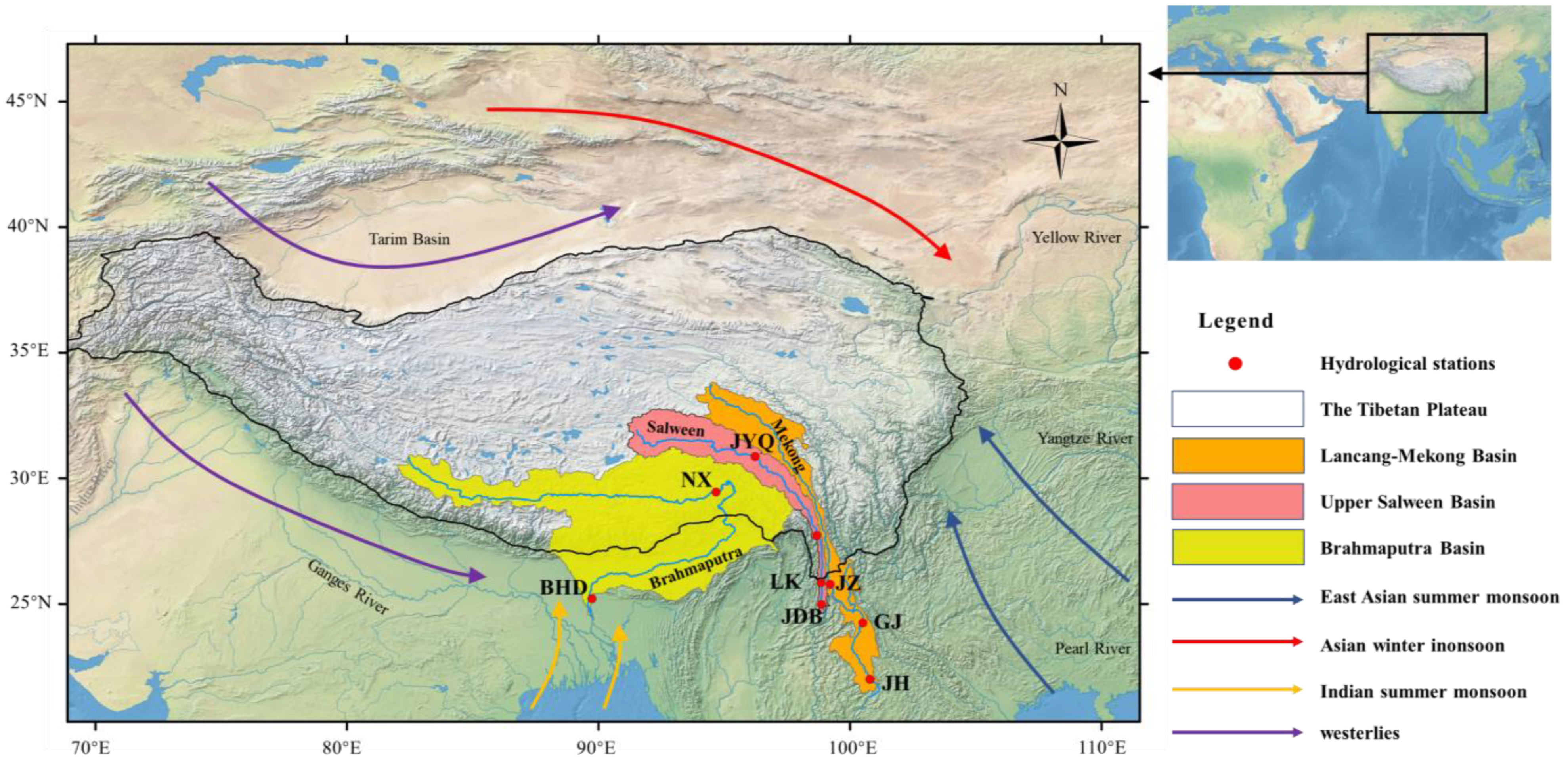
Figure 1. The location of the study area, regional river basins, hydrological stations and major monsoon and wind systems. Hydrological stations are JiuZhou (JZ), Gajiu (GJ), Jinghong (JH), Liuku (LK), Jiayuqiao (JYQ), Jiedaoba (JDB), Gongshan (GS), Nuxia (NX) and Bahadurabad (BHD).
Hydrology 12 00218 g001
Figure 2. Systematic bias distribution of ECMWF ENS extended forecast in a total of 13 years, 2008–2020.
Hydrology 12 00218 g002
Figure 3. The area ratio of the region with systematic bias.
Hydrology 12 00218 g003
Figure 4. Mean frequency of overestimating.
Hydrology 12 00218 g004
Figure 5. The logarithm of the mean correction factor (with a base of 10).
Hydrology 12 00218 g005
Figure 6. The time series of the correction factor at (a) Nuxia; (b) Bahadurabad.
Hydrology 12 00218 g006
Figure 7. Mean bias before and after correction in calibration and validation period.
Hydrology 12 00218 g007
Figure 8. The mean bias on each grid before and after correction during the validation period.
Hydrology 12 00218 g008
Figure 9. The hydrological forecasting performance at hydrological stations before and after correction of precipitation bias during (a) calibration period; (b) validation period.
Hydrology 12 00218 g009
Figure 10. Monthly aggregated relative error of total water volume at hydrological stations before and after correction of precipitation bias during (a) calibration period; (b) validation period.
Hydrology 12 00218 g010
Figure 11. Improvement effect and improvement frequency of different methods for determining the correction factor. * Note that the “mean” in the figure refers to the correction factor calculated using Equation (3), not the average of the correction factors.
Hydrology 12 00218 g011
Table 1. Daily-scale calibration and validation performance of the THREW model for specific stations across three study basins.
BasinCalibration PeriodValidation PeriodStationsNSE
CalibrationValidation
Upper Mekong1991–20002001–2009Jiuzhou0.790.82
Gajiu0.810.79
Jinghong0.830.81
Salween2000–20082009–2020Daojieba0.820.83
Liuku0.780.82
Gongshan0.770.73
Jiayuqiao0.750.73
Brahmaputra1983–20002001–2015Nuxia0.780.79
Bahadurabad0.870.80
Table 2. Mean relative error and improvement frequency in hydrological forecasting before and after correction of precipitation bias.
BasinStationsCalibration PeriodValidation Period
Mean Relative Error (%)IF (%)Mean Relative Error (%)IF (%)
BeforeAfterBeforeAfter
Upper MekongJiuzhou20.099.9384.1418.0410.0777.89
Gajiu21.369.9882.9118.919.8274.61
Jinghong16.439.2676.1419.649.5865.22
SalweenDaojieba10.885.9877.889.715.2469.60
Liuku11.196.3076.1910.526.8168.20
Gongshan8.685.6471.428.455.9166.59
Jiayuqiao8.886.2573.018.176.0265.64
BrahmaputraNuxia25.329.5891.4920.439.4585.72
Bahadurabad20.378.3688.1821.0810.4382.66
Disclaimer/Publisher’s Note: The statements, opinions and data contained in all publications are solely those of the individual author(s) and contributor(s) and not of MDPI and/or the editor(s). MDPI and/or the editor(s) disclaim responsibility for any injury to people or property resulting from any ideas, methods, instructions or products referred to in the content.