Precipitation-Related Atmospheric Nutrient Deposition in Farmington Bay: Analysis of Spatial and Temporal Patterns

Abstract

This study quantifies the atmospheric deposition (AD) of nutrient loads into the Farmington Bay ecosystem via wet deposition over a three-year period. We analyzed nutrient concentrations from 509 total phosphorus (TP), 507 orthophosphate (OP), and 511 total nitrogen (TN) samples collected at seven locations around the Bay. We estimated AD loads using two different spatial interpolation methods, Kriging and Inverse Distance Weighting (IDW), as well as average concentrations. The loads computed using Kriging and IDW were similar, but the loads computed using sample averages were about 70% smaller. We estimated that annual atmospherically deposited nutrient loads range from 306 to 594 Mg for TN, 73 to 195 Mg for TP, and 43 to 144 Mg for OP. The loads in 2023 were significantly higher than those in 2021 and 2022, a phenomenon we attribute to higher precipitation and a major loading event that occurred on 13 April 2023. Based on comparison with studies concerning nearby Utah Lake, the total loads could be two to three times larger than our estimates. These studies suggest that fine particulate matter may significantly contribute to AD nutrient loads, but these loads are not captured by our sampling method. However, the inclusion of non-water surfaces in Farmington Bay may mitigate this difference.

1. Introduction

1.1. Atmospheric Deposition of Nutrients into Lakes and Reservoirs

Total phosphorus (TP), orthophosphate (OP) content, and total nitrogen (TN) are important nutrients and are often measured in aquatic ecosystems to assess their health. TP and TN represent all phosphorus and nitrogen forms within a sample, including those present in algae and sediment particles, providing an integrated view of the available nutrients in the sample [1]. OP is the inorganic form of dissolved phosphorus, consisting of orthophosphate ions—mostly ${\mathrm{P}\mathrm{O}}_4^{3-}$. These ions are crucial for ecosystems as they are the only form of phosphorus that plants can directly use for growth. OP is typically derived from the mineralization of organic matter, and it is a key indicator of nutrient availability in aquatic environments [2].

Excess TN and TP inputs from anthropogenic and natural sources can trigger eutrophication in aquatic systems, facilitating harmful algal blooms (HABs) with substantial ecological and economic repercussions. These phytoplankton proliferations significantly disrupt aquatic ecosystem structure, leading to biodiversity declines and compromising regional biological resources. Some HABs involve the growth of toxin-producing cyanobacteria that can create dangerous conditions for humans and wildlife [3].

Nutrient loadings of TP, OP, and TN from atmospheric deposition (AD) are potentially significant sources of nutrients for aquatic ecosystems [4,5,6]. Hillary et al. [5] noted that research on air pollution and acidic deposition has significantly advanced our understanding of atmospheric deposition rates and processes in recent years and that these processes are important for understanding aquatic systems. Atmospheric deposition should not be underestimated as a significant source of nutrients and a potential driving force of eutrophication [7].

AD can be very episodic, and a significant portion of the total load occurs during discrete events [8]. Wet deposition associated with precipitation events can be both episodic, based on atmospheric particles and rainfall events, and spatially and temporally heterogenous [8,9]. Studies of AD with respect to the Mediterranean Sea have shown that only a few intense events provide the bulk of the annual load [10,11]. Studies have documented short-term events, on the order of a few hours, having fluxes on the order of 20 g/m² [12,13,14].

Three recent studies of AD in Utah Lake, which is located along the Wasatch Front about 50 km south of Farmington Bay, documented nutrient loads using two different measurement methods. Two studies measured both bulk and dry deposition in Utah Lake: The first estimated total AD loads of 320 and 140 Mg/year TP and 420 and 460 Mg/year of dissolved inorganic nitrogen (DIN) for 2017 and 2018, respectively [15]. In the second study, updated collection methods were used, and the researchers estimated 240 and 120 Mg/year of TP and 955 and 440 Mg/year of DIN for 2019 and 2020, respectively [16]. Assuming the average area of Utah Lake is 38,000 hectares [17], these are TP deposition rates of approximately 0.84, 0.34, 0.63, and 0.32 g/m²/year and DIN deposition rates of 1.1, 1.2, 2.5, and 1.2 g/m²/year for 2017, 2018, 2019, and 2020, respectively [15,16].

A third Utah Lake study estimated annual AD rates only based on precipitation events over a 5 year period: the rates for TP, OP, and TN were 120 Mg/year, 61 Mg/year, and 435 Mg/year, respectively [17]. Brown et al. [17] estimated that AD from precipitation sources contributes between 25% and 40% of the total AD nutrient load. Brown et al. [17] collected data on precipitation after events, measured nutrient concentrations in the collected samples, and used rain gage data to estimate the total storm volume on the lake. The nutrient loadings were estimated by multiplying the measured concentration by the precipitation volume.

Brown et al. [17] separated AD into three categories to match the field conditions used in their study and previous Utah Lake studies [15,16]. These categories used to classify AD are based on the different deposition processes (which are analyzed using different sampling methods): settlement (dust), contact (suspended, small particles), and precipitation (or washout). These categories do not follow the categories from traditional AD research, in which two categories and a combined category are commonly used: wet (gases washed out during precipitation), dry (settled dust and particulates), and bulk (a combination of the wet and dry processes).

We follow the categories used by Brown et al. [17], which separate precipitation AD from AD through other sources, because we followed their field collection methods. These methods generally capture particles in the atmosphere during precipitation but do not include fine dust deposition outside of precipitation events. This is different from the bulk or wet deposition definitions commonly used in the AD literature. Brown et al. [17] provide more detailed descriptions of these categories. This approach directly measures wet deposition, but because of the design of the samplers, they capture little dry deposition and no small particulate deposition. Brown et al. [17] concluded that the AD nutrient loads estimated using precipitation measurements are between 25% to 40% of those estimated using sampling procedures that capture all three categories, i.e., settlement (dust), contact (small particles), and precipitation, in a study pertaining to Utah Lake, a lake located about 50 km south of Farmington Bay, with similar environmental and AD conditions.

1.2. Farmington Bay of the Great Salt Lake

This study focuses on Farmington Bay, which is part of the Great Salt Lake in Utah, USA. Farmington Bay functions as a receiving basin for municipal and industrial wastewater from the major urban areas of Davis and Salt Lake counties while also collecting non-point source pollution from agricultural and urban runoff. Previous research has extensively documented various aspects of the dynamics of the Farmington Bay ecosystem, including nutrient fluxes within the bay and the movement of groundwater through sediment pore spaces [18]. Anthropogenic impacts have been thoroughly investigated through comprehensive metal analyses [19], while numerous studies have focused on the bay’s eutrophication status, limnological characteristics [20], and chlorophyll concentrations [21]. Investigations have evaluated the effects of various processes on aquatic life and migratory bird populations that depend on this ecosystem [22].

While researchers have conducted detailed analyses of TP, OP, and TN loads from sewage discharged into Farmington Bay and concluded that approximately 50% of nutrients going into the Bay come from sewage treatment plants [23], there remains a significant gap regarding the contribution of AD to these nutrient loads. We attempt to address this critical research gap by specifically examining atmospheric deposition of TP, OP, and TN nutrients, which have not been previously investigated in the Farmington Bay ecosystem.

1.3. Study Overview

The aim of this study was to quantify and assess the precipitation-related AD rates of TP, OP, and TN in Farmington Bay, Great Salt Lake, from 2021 to 2024 using the sample collection methods reported by Brown et al. [17]. We collected nutrient concentration data from seven sampling stations around Farmington Bay, and we accessed precipitation data from seven meteorological stations and wind data from four anemometer stations. We employed and compared two different spatial interpolation techniques, namely, Kriging and Inverse Distance Weighting (IDW), to generate areal distributions of concentration and precipitation and used these distributions to compute the nutrient AD loads.

Here, we present a comprehensive analysis of TP, OP, and TN loads from precipitation-related AD in Farmington Bay. We provide a detailed investigation of the relationships between the nutrient concentrations measured and environmental factors, including precipitation patterns, wind conditions, and atmospheric pollution. We discuss the episodic nature of the data and show how single deposition events can provide significant loads, contrary to the common assumption that AD provides a steady but small inflow of nutrients. This is in line with the AD literature, which shows that single events can provide a significant portion of AD loads [24,25].

This research addresses two primary questions: (1) what are the spatial and temporal patterns of AD for TP, OP, and TN in Farmington Bay, and (2) how do precipitation patterns, wind characteristics, and pollutants in the environment influence the AD of these nutrients? We provide estimates of total annual loads for the three years studied. These estimates can provide resource managers with information that can inform decisions on nutrient impacts and mitigation.

This investigation provides valuable insights into nutrient deposition dynamics in Farmington Bay, informing water quality management strategies by providing a better understanding of the atmospherically deposited loads in the Bay. This study also contributes to the understanding of nutrient loads in similar lake ecosystems. AD loads are often neglected or assumed to be minimal, and this study shows that AD can provide significant nutrient loads to water systems.

Characterizing and understanding nutrient AD loads is an important issue for evaluating the environmental impacts on aquatic ecosystems and a nutrient load source that is often overlooked. AD can provide significant nutrient loads to water bodies, contributing to processes like eutrophication, which disrupts ecological balance and harms aquatic life [16,17,25]. Studies focused on nutrient AD loads provide critical insights into episodic deposition events and their role in shaping nutrient dynamics, revealing that these events often deliver substantial nutrient loads that are overlooked in steady-state assumptions [6,7,13]. Since AD sources can make a significant contribution to total nutrient loads, this information is helpful for resource managers, enabling them to developed strategies for mitigating nutrient pollution, preserving water quality, and managing the ecological health of sensitive ecosystems like Farmington Bay.

This study has broader applicability to other water bodies that are impacted by excess nutrients. We present methods involving the use of spatial interpolation, precipitation sampling for nutrient concentration, and precipitation volumes that allow researchers and managers to uncover the patterns and drivers of nutrient deposition across aquatic environments. These findings provide better information on total nutrient loads that can inform management strategies for lakes, rivers, and coastal systems experiencing similar challenges. Understanding AD nutrient loads enhances our ability to predict and mitigate anthropogenic impacts, contributing to the global effort to sustain aquatic ecosystems and their vital functions for biodiversity and human livelihoods.

2. Study Area, Data, and Methods

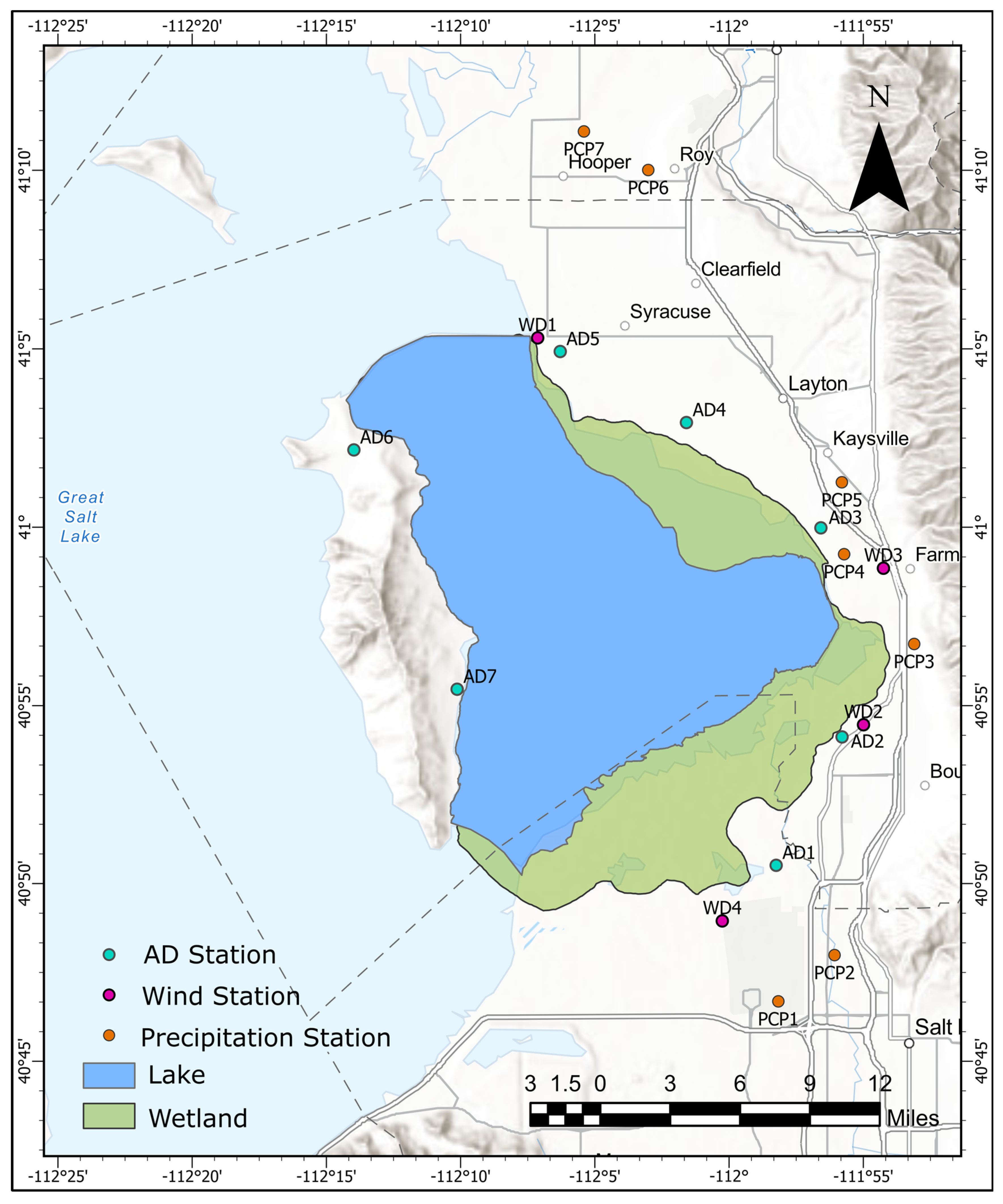
2.1. Farmington Bay Area

Our study area is Farmington Bay, one of the 5 bays of the Great Salt Lake, located in the Southeast portion of the lake. The geographical boundary for Farmington Bay is defined by the Utah Administrative Code (R317-2-6) for beneficial use category 5D for Water Quality. This legal description notes that Farmington Bay includes all open water at or below approximately an elevation of 4208 feet (1282.6 m) east of Antelope Island and south of the Antelope Island Causeway.

In our study, we limited the boundary on the Southwest section to a dike connecting the mainland to Antelope Island’s southernmost tip, as shown in Figure 1. To precisely delineate this area, we traced a contour of the Great Salt Lake’s bathymetry in raster format using data provided by a HydroShare resource [26]. These data were created by mosaicking multiple elevation datasets, including the National Elevation Dataset (NED) Digital Elevation Module and field survey data [26]. From this elevation dataset, we extracted a boundary corresponding to the 4208-foot elevation contour. We further divided the study area into two distinct zones based on flooding frequency or lake level: a water area, comprising regions subject to seasonal inundation as defined by the Utah Geological Survey (UGS) wetland classification, which is the blue area in Figure 1, and a wetland area, shown as the green area in Figure 1, which encompasses the remaining regions classified by UGS as intermittently flooded. The water area is 325 km², and the wetland area is 165 km², together amounting to a total area of 490 km². Figure 1 shows AD concentration, precipitation, and wind measurement stations.

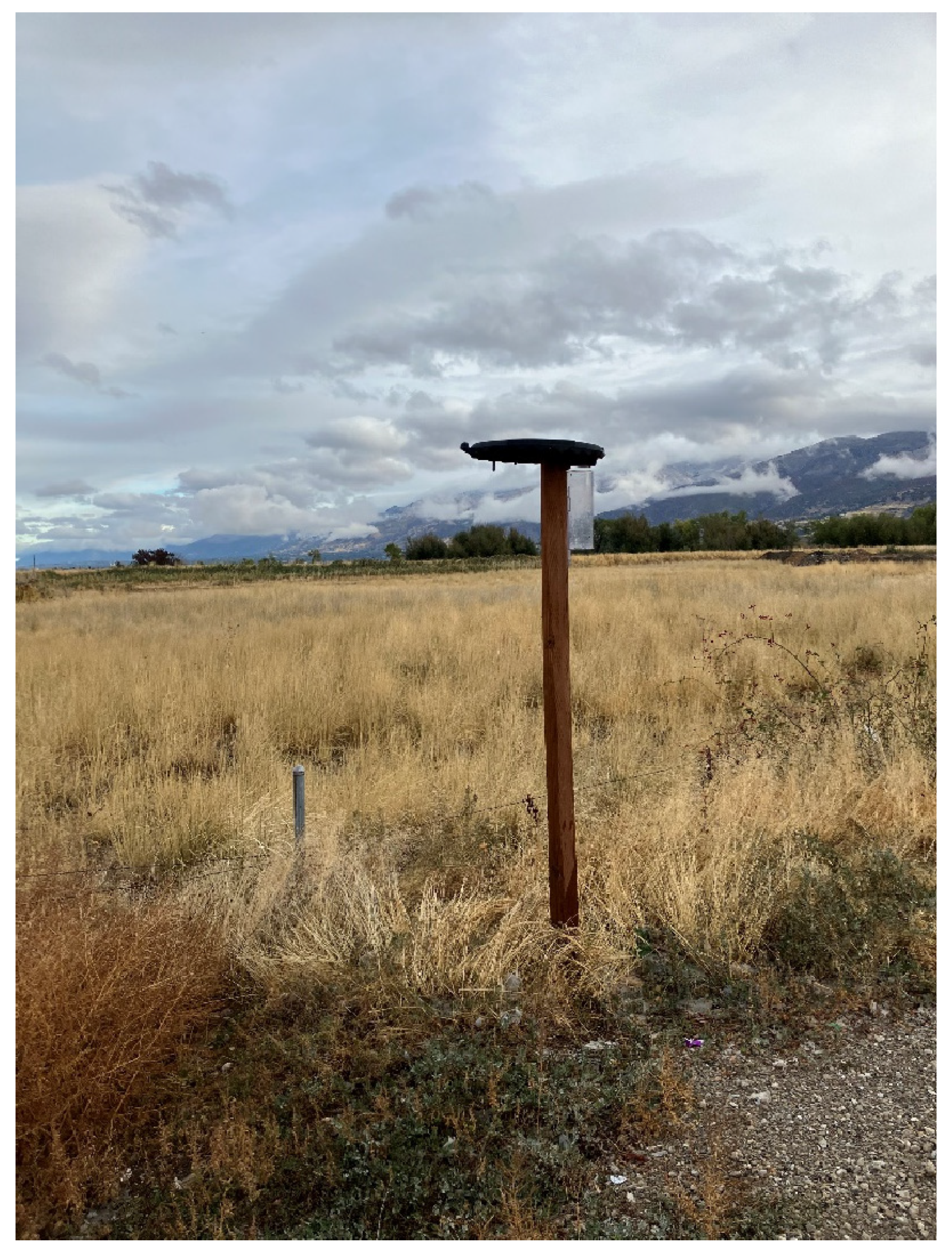
2.2. AD Sample Collection

We established sampling stations (AD stations) at 7 locations around Farmington Bay (Figure 1). A picture of one of the sampling stations is shown in Figure 2. The samplers are designed to capture precipitation but not AD from dry or particulate depositions. The design of the samplers was replicated based on the study by Brown et al. [17]. We collected water from these stations after each rainfall event from 13 March 2021 to 7 January 2024. This effort resulted in 509, 507, and 511 measurements of TP, OP, and TN, respectively. The names and locations of the sampling stations are presented in

Table 1. Atmospheric-monitoring stations surrounding Farmington Bay, Utah.

Station Index	Name	Latitude	Longitude
AD1	Gillmor Farm	40.842	−111.971
AD2	South Davis	40.902	−111.930
AD3	Central Davis	41.000	−111.943
AD4	GSL Preserve	41.049	−112.026
AD5	North Davis	41.082	−112.105
AD6	Buffalo Pens	41.036	−112.233
AD7	Garr Ranch	40.924	−112.169

and shown in Figure 1 as green dots.

We collected samples typically the day after storm events, with only minor deviations from this protocol, in order to reduce potential sample evaporation, as this method measures concentrations. We examined samples for issues such as bird droppings or dead insects. The samples were generally clear, showing no visible contamination. We transported the samples in sealed bottles. We cleaned the samplers after each sample collection phase.

The samplers do not generally retain dry dust depositions from larger particles, as these dry particles are easily resuspended by wind and blown from the surface, though some become trapped in the container. These samplers do not collect appreciable quantities of very small particles (<10 µm) that are suspended in the atmosphere and deposited in water bodies through contact with the water surface. Thus, the nutrients in the samples mostly stem from precipitation AD, with some smaller portions stemming from settlement (dust) and contact (fine particulate matter). We attribute the loads estimated from these samples to “precipitation AD loads”, though there are minor contributions from settlement and contact deposition processes.

Chemtech-Ford Laboratories, a TNI-accredited environmental testing facility, analyzed samples for TP, OP, and TN concentrations, with results reported in milligrams per liter (mg/L). They used EPA methods 200.7 and 353.2 for TP and TN, respectively (www.epa.gov), and SM45000 P-E/F Phosphorus by Ascorbic Acid (Ascorbic Acid Method) Standard Methods Online, National Environmental Methods Index (NEMI) (https://www.nemi.gov/methods/method_summary/7436/, accessed on 13 March 2025). The detection limits were 0.007 mg/L for TP and OP and 0.1 mg/L for TN. Samples with concentrations below these limits were reported as below detection limit (BDL) by the instrument. For the analysis purposes of this study, we replaced the reported BDL values with half of the detection limits.

2.3. Precipitation Data Source

We acquired daily precipitation data from three different networks, namely, Community Collaborative Rain, Hail, and Snow Network (CoCoRaHS); Global Historical Climatology Network (GHCN); and Meteorological and Climatological Historical Database (MCHD), all downloaded from (https://climate.usu.edu/swco/. Accessed on 10 September 2024). We selected stations that had precipitation data for the duration of the study period. We further screened the stations based on their locations. We did not include stations too far away from Farmington Bay, stations near the mountains (which received a different precipitation pattern), and those very near the urban areas, resulting in 10 candidates. We discovered that two of these stations had a significant number of missing values. Additionally, in some cases, the reported data showed a meaningful difference from the average precipitation data for other stations, so we did not use these stations. Through this process, we selected 7 precipitation stations, shown in Figure 1 as orange dots, with details in

Table 2. Precipitation monitoring stations surrounding Farmington Bay, Utah.

Station Index	Station Name	Latitude	Longitude	Elevation (m)	Network
PCP1	Salt Lake City Intl Ap	40.778	−111.969	1288	GHCN
PCP2	Rose Park	40.800	−111.935	1287	MCHD
PCP3	Centerville 1.3 N	40.945	−111.885	1300	CoCoRaHS
PCP4	Farmington 1.8 W	40.987	−111.929	1292	GHCN
PCP5	Kaysville—USU Farm	41.021	−111.930	1372	MCHD
PCP6	Eagle Lake	41.167	−112.050	1334	MCHD
PCP7	West Haven 2.0 SW	41.185	−112.090	1292	GHCN

.

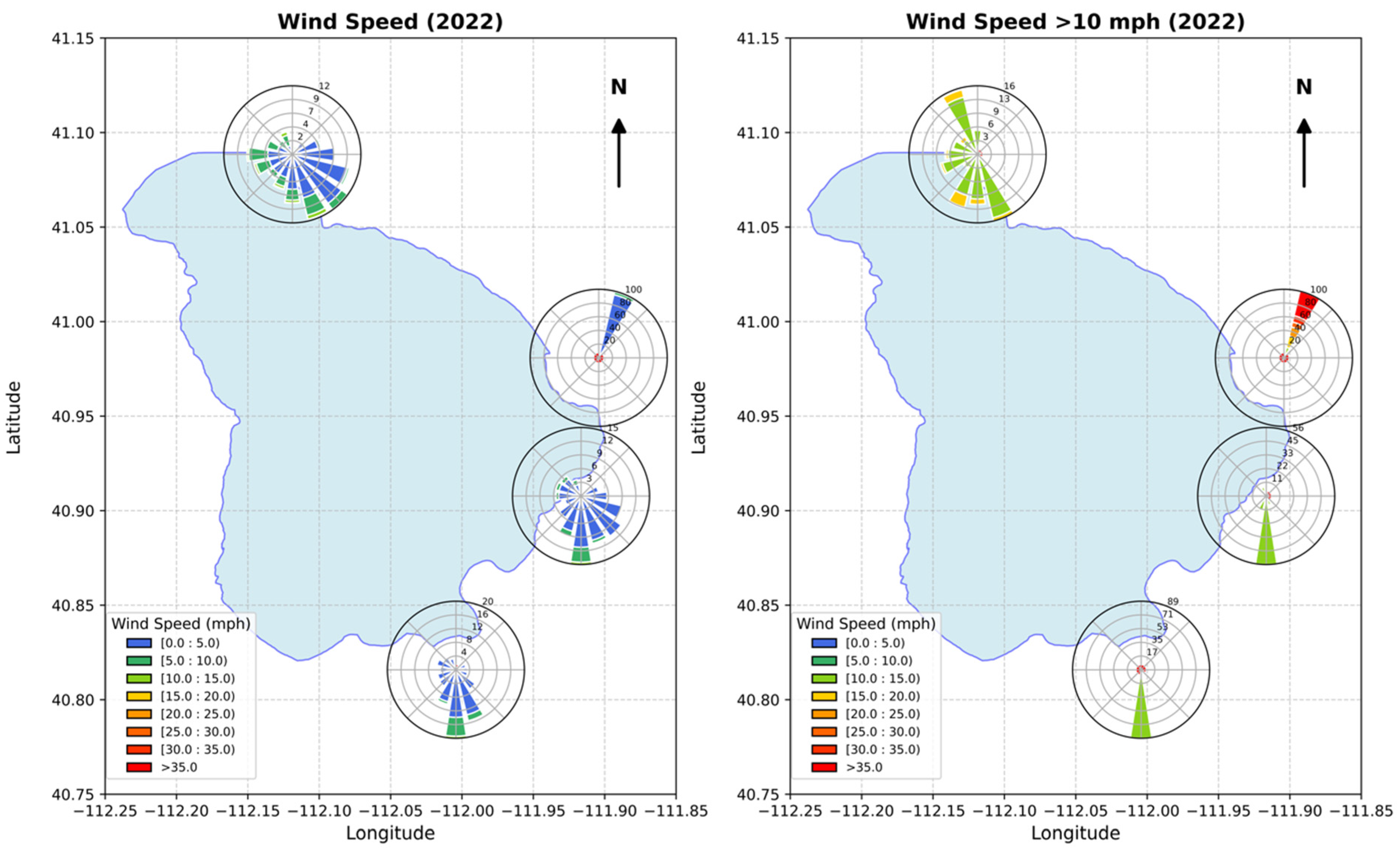
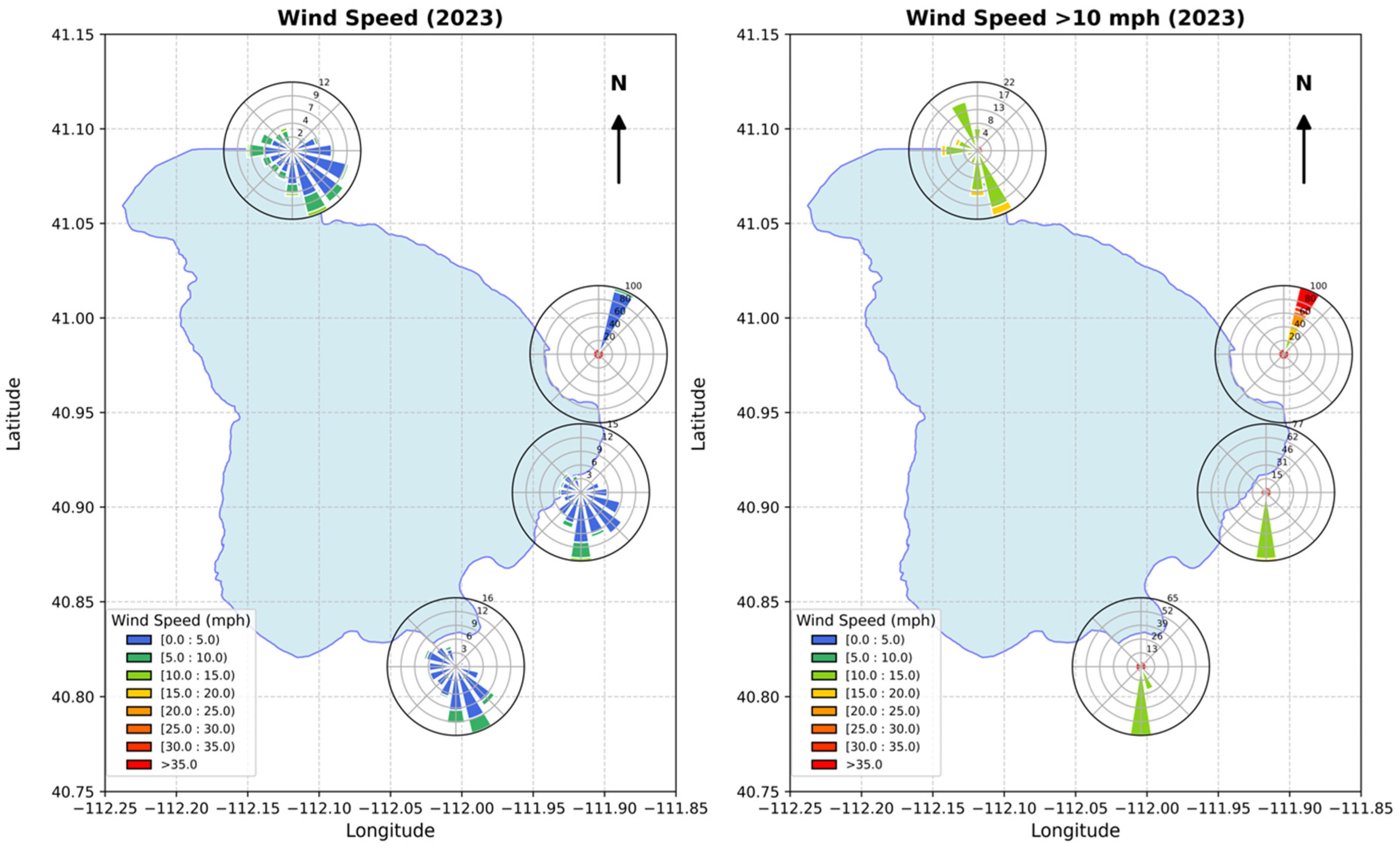
2.4. Wind Data Sources

We obtained wind data from the MESOWEST network (https://climate.usu.edu/swco/. Accessed on 16 October 2024) for stations across the study area. Of the seven initially identified stations, we excluded three: the two near Gillmor Farm and Buffalo Pens, which lacked complete wind data for the study period, and a third that was located too far from the primary area. We selected four wind stations (Figure 1 and

Table 3. Wind stations used in this study.

Station Index	Station Name	Station ID	Latitude	Longitude	Elevation (m)	Network
WD1	Syracuse	UUSYR	41.088	−112.119	1285	MESOWEST
WD2	Legacy Parkway	UTLGP	40.908	−111.917	1284	MESOWEST
WD3	KJ7NO-2 Farmington	AP611	40.981	−111.904	1290	MESOWEST
WD4	SLC Airport Wind 2	SLCNW	40.816	−112.004	1304	MESOWEST

) with continuous, sub-hourly interval measurements and no missing data during the study period for our analysis.

2.5. Air Quality

Fine particulate matter measured for health considerations is classified based on a particle’s aerodynamic diameter. Particles with diameter less than 2.5 µm are classified as PM2.5, and those less than 10 µm in diameter are classified as PM10 [27]. PM2.5 particulates typically originate from sources such as the combustion of fossil fuels, biomass burning, transportation, and industrial processes, whereas PM10 particulates typically originate from mobilized soil or dust from processes and locations such as construction sites, landfills, unpaved roads, and agricultural activities [27,28]. Particulates, especially PM2.5, can be formed in the atmosphere through chemical reactions of different gases [27].

In AD studies, these particulates play a crucial role, as PM2.5 has been known to contribute to TP and OP, and the same is true for PM10 with respect to TN. We accessed Environmental Protection Agency (EPA) air quality data for the study area to evaluate correlations with measured AD patterns (https://www.epa.gov/outdoor-air-quality-data/download-daily-data. Accessed on 3 November 2024).

2.6. Load Calculation

We used and compared two different methods, ordinary Kriging and IDW, for performing spatial interpolation of both concentration and precipitation data for use in calculating nutrient loads. Ordinary Kriging and IDW are similar: estimated values at a point are computed using a weighted average of all the measured data. The difference lies in how the weights are computed. In both methods, it is assumed that the measured values are more similar to values measured at nearby locations. In IDW, it is assumed that measured values, no matter hows far away, influence the estimated value, though weights drop off quickly with distance. In Kriging, it is assumed that there is a range beyond which measured values do not influence the estimated value and that the best estimate is the average value. Kriging has an advantage: in addition to computing an estimated value, it also computes an uncertainty measure for each estimate. In either method, the interpolated value is most influenced by the nearest measured value.

Both methods can be expressed as follows:

$$S_0=\sum _{i=i}^n{\lambda }_i{S}_i$$

(1)

where $S_i$ is the $i$ measured value at location $S_i$, $S_0$ is the estimated value at location $S_0$, ${\lambda }_i$ is the weight for the measurement, and n is the number of measured values.

In IDW, ${\lambda }_i$, which is the weight for a given measurement, is based on the distance to the estimated location from each of the measured values, computed as

$${\lambda }_i={\displaystyle \frac{d_i^{-\alpha }}{\sum _{i=1}^n{d}_i^{-\alpha }}}$$

(2)

where $d_i$ is the distance between the location of the measured value $S_i$ and the location to be predicted, $S_0$, and α is the weighting factor. For our work, we used $\alpha =2$, i.e., inverse distance squared.

In Kriging, the weights are based both on the distance from the measurement to the prediction location and a function that captures the range of influence among the data—or the distance over which we would expect values to be influenced by nearby measurements. This is quantified using a spatial autocorrelation function fitted to the semi variance of the data. We chose to use a spherical variogram model as the distance-weighting function. A spherical variogram was defined:

$$\gamma \left(h\right)=\left\{\begin{array}{cc}{c}_0+c\left({\displaystyle \frac{3h}{2a}}-{\displaystyle \frac{1}{2}}\left({\displaystyle \frac{h^3}{a^3}}\right)\right)& 0<h\le a\\ c_0+c& h>a\\ c_0& h=0\end{array}\right.$$

(3)

where $\gamma \left(h\right)$ is the semi variance at distance $h$; $c_0$ is the nugget, or variance at a distance of 0; c is the sill or maximum variance; and a is a fitting parameter related to the range of the variogram or the distance over which values are related to each other.

The maximum distance between the stations is 30.78 km. For the variogram, we set the range to 30% of this value, which is about 9.26 km. We selected zero as the nugget value and set the sill equal to the standard deviation of all measured concentrations or precipitation for each nutrient or rainfall value.

2.7. Analysis Overview

We used the two methods to spatially interpolate the precipitation and each nutrient concentration value onto a grid with a spacing of 25 m × 25 m that covered both the lake area and the wetland area. For each day for which we had nutrient measurements, we generated a grid of interpolated values. We summed the daily precipitation values from the day following the preceding nutrient-sampling date to the day of the next sampling date. This resulted in the total amount of precipitation observed since the last nutrient measurement. Generally, there was only the precipitation event related to the nutrient sampling event as we attempted to collect samples after each event. However, in some cases, we summed multiple recorded precipitation events.

This resulted in two sets of grids or rasters for each nutrient-sampling event. One set was the estimated concentration at each grid square of each nutrient (mg/L), and the second was the estimated precipitation amount at each grid square for each nutrient-sampling event (mm).

To compute the loads, we multiplied the precipitation raster by the area of each grid, 625 m², to obtain volume; then, we multiplied each precipitation volume raster and each nutrient concentration (mg/L) and used a conversion factor of 10⁻⁶ to obtain AD loads for each nutrient for each grid square in kilograms/grid-square. We clipped the raster with the lake boundary and wetland boundary to extract the respective AD values for these two areas.

To obtain the total load per event, we summed the raster values. This gave us a total kg of load for each nutrient for the selected area. For annual loads, we summed the event loads by year. For reporting, we converted these values from kg to Mg (1000 kg).

3. Data Analysis

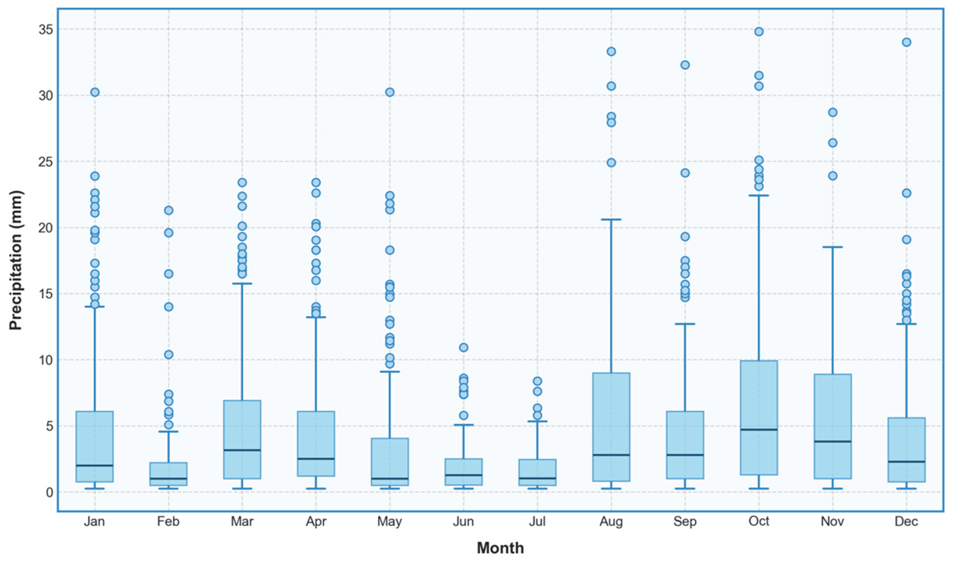
3.1. Precipitation Data Analysis

Figure 3 shows the distribution of daily precipitation for each station over the study period. The rainfall amounts are similar across all stations, though stations PCP3 and PCP4 have slightly higher median values, which is expected as they are nearer to the mountains. The windward slope of the Wasatch Range receives more rainfall than the valley floor. All the stations have some outliers, but the daily measured precipitation does not exceed 35 mm at any station.

Figure 4 shows the distribution of precipitation by month over the study period. There is a seasonal pattern, with the summer season (June to August) being the driest period and precipitation beginning to increase in August. This occurs due to the meteorological phenomenon wherein Utah experiences isolated and intense rainstorms in the late summer [29]. This occurs due to the movement of moisture-laden air masses from the Gulf of Mexico. The data show higher precipitation in late summer and fall (September to November), peaking around October, with a relatively consistent precipitation pattern throughout the Winter and Spring before decreasing during summer, though February consistently has lower precipitation than January or March.

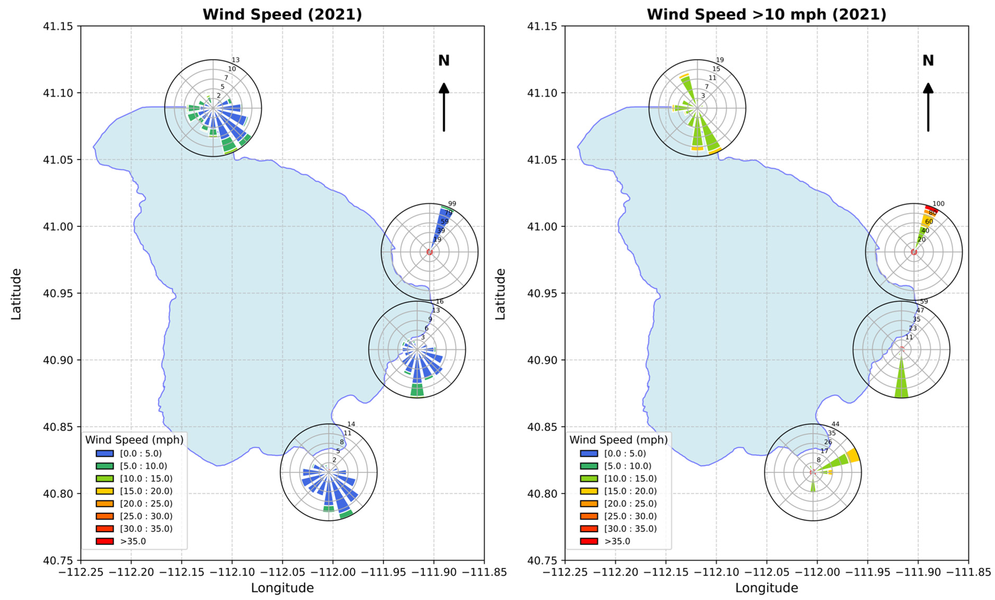
3.2. Wind Data Analysis

To characterize wind patterns, we constructed two different wind rose diagrams: one using all the available data for each year and another showing the prevailing directions of the higher-speed winds using only data for wind speeds above 10 miles per hour (mph) (4.5 m/s), as high wind speeds are more likely to mobilize and deposit dust. Wind data for 2021 are presented in Figure 5. Data from 2022 and 2023 are presented in Figure A1 and Figure A2, located in the Appendix A. The figures show wind roses with all the data in the left panel and only winds above 10 mph (4.5 m/s) in the right panel.

Prevailing wind directions vary significantly around Farmington Bay. The highest wind speeds occur at Station WD3, the northern station on the east side of the Bay (Figure 1). This station is closer to the mountain front and is most likely influenced by canyon winds. The prevailing wind direction and the direction of the winds over 10 mph (16 km per hour) are both from the northeast with slight variation, which is unusual; we attribute this constant direction to influence from the canyons. The two stations midway up the eastern shore, WD2 and WD3 (Figure 1), have prevailing high winds (Figure 5, right panel) nearly opposite each other. The station at the Salt Lake airport, WD4, has high-speed winds (Figure 5, right panel) from the northeast that occur rarely, with prevailing winds (Figure 5, left panel) from the southeast. However, the winds from 2022 and 2023 (Appendix A Figure A1 and Figure A2) have different patterns, with the high-speed winds blowing in from the South in both years. The station on the northeast corner of the Bay WD1 (Figure 1) has variable winds, with the prevailing direction for the higher winds being similar to the general wind rose. In the next section, we attribute some of the variability in the data to these varying wind directions and speeds in different areas of the Bay. Wind direction influences ADtransport, and higher wind speeds can mobilize dust and other particulate matter.

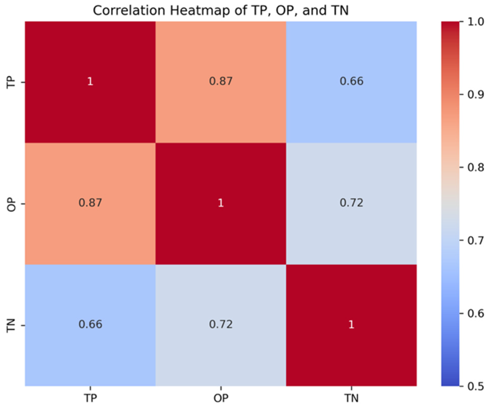
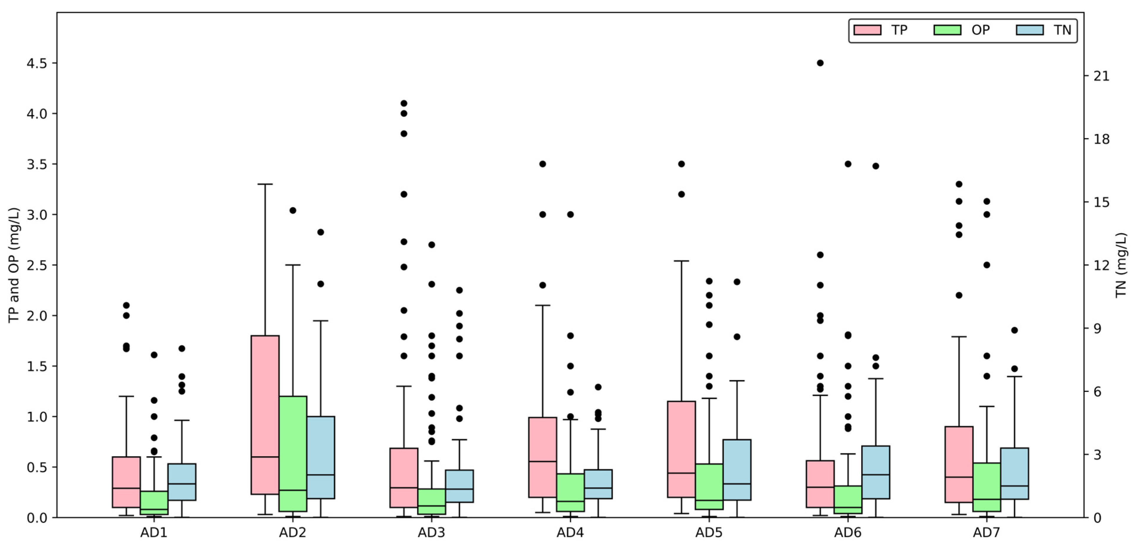
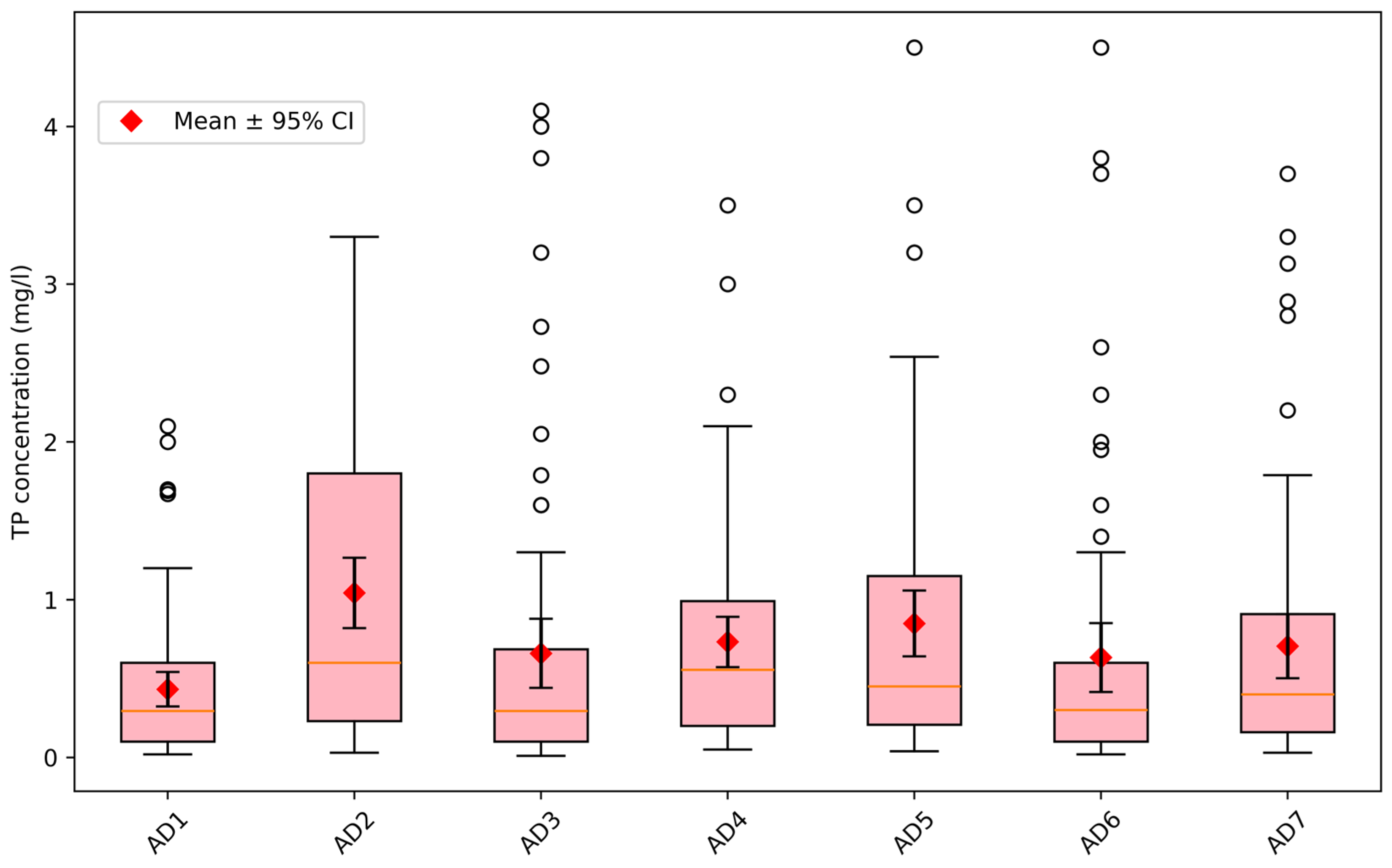
3.3. Nutrient Concentration Data

Table 4. Statistical summary of nutrient concentration data.

Nutrient	Station Index	Number of samples	Mean (mg/L)	Median (mg/L)	Max (mg/L)	Skew
TP	AD1	74	0.43	0.30	2.10	1.88
	AD2	73	1.04	0.60	3.30	0.80
	AD3	74	0.66	0.30	4.10	2.29
	AD4	74	0.73	0.55	3.50	1.72
	AD5	74	0.85	0.45	4.50	1.77
	AD6	70	0.63	0.30	4.50	2.52
	AD7	70	0.71	0.40	3.70	1.89
OP	AD1	74	0.21	0.08	1.61	2.51
	AD2	73	0.67	0.27	3.04	1.09
	AD3	74	0.35	0.11	2.70	2.36
	AD4	74	0.34	0.16	3.00	3.09
	AD5	73	0.42	0.17	2.34	1.98
	AD6	68	0.34	0.10	3.50	3.27
	AD7	69	0.43	0.18	3.13	2.64
TN	AD1	73	1.90	1.60	8.03	1.73
	AD2	74	3.24	2.04	13.56	1.34
	AD3	75	2.14	1.40	12.90	2.49
	AD4	74	1.79	1.40	6.20	1.24
	AD5	73	2.37	1.60	11.20	1.60
	AD6	71	2.82	2.11	16.70	2.65
	AD7	70	2.53	1.55	13.70	2.00

summarizes the nutrient concentration data collected at each station. The information includes the number of samples analyzed for each nutrient at each station; the mean, median, and maximum values; and the skew of the data. Depending on the station, we collected between 70 to 74 TP samples, 68 to 74 OP samples, and 70 to 75 TN samples at the seven AD measurement stations (Table 4).

The OP data are the most skewed, with a mean skew value of 2.4 and two stations, AD4 and AD6, presenting skew values over 3. The mean skew values for the TN and TP data are similar, amounting to 1.86 and 1.84, respectively. The two stations with the most skewed data for all three nutrient concentrations are AD3 and AD6, with AD3 located about midway up the eastern side of the Bay and AD6, the northern station on Antelope Island, being on the west side (Figure 1). This might be somewhat explained by the wind data, as the winds at the northwest of the Bay near AD6 are the most varied (Figure 5), while the wind roses for the stations on either side of AD3 show prevailing winds almost 180 degrees away from each other (Figure 5).

Figure 6 presents concentration data as box plots and histograms for each nutrient with the data aggregated from all the stations. The TN data have a higher concentration range and more extreme outliers compared to the TP and OP data. The TN data display the widest interquartile range, indicating greater variability, while TP and OP have lower median concentrations and fewer extreme values. Both the TP and OP values exhibit clustering around lower concentrations, with a few high outliers. The distributions of all three nutrients are skewed right, as indicated by the skew values, with most values lying towards the low end of the range, but all exhibit significant tails at higher concentrations, with a few high values occurring for each of the different nutrients.

Figure 7 shows a strong positive correlation between TP and OP (0.87), indicating they generally increase and decrease together, as expected. TN is positively correlated with both TP (0.66) and OP (0.72), though the correlation is slightly weaker. The measured concentrations of the three nutrients are positively correlated with each other, suggesting they share common sources or processes that influence concentrations. We expected the nutrient concentrations to be correlated, as we hypothesize that nutrient loads are a function of the concentration of particulates in the atmosphere at the time of a precipitation event.

Figure 8 presents distributions of all three nutrients organized by sampling station. The TN concentrations are consistently higher and more variable than the TP or OP concentrations. The Central Davis (AD3) sampling station has the largest number of TN outliers, showing frequent spikes in nitrogen concentration, though the central distribution, median, and mean values are lower than those for most of the other stations. South Davis (AD2) has the largest median and mean values along with the largest range in TN concentrations, indicating higher TN deposition concentrations possibly linked to nearby sources. In contrast, the TP and OP levels exhibit a more similar distribution across the sampling sites, with fewer outliers, pointing to less variation in phosphorus concentrations. As with TN, South Davis (AD2) has higher mean and median TP and OP concentration values than the other stations. The lowest concentrations for all three nutrients occur at Gillmor Farm (AD1). The remainder of the stations are similar to each other.

Phosphorous is of particular concern for eutrophication in Farmington Bay. To better understand the spatial distribution and compare the concentrations at the different sampling locations, we created Figure 9, which presents the distribution of only the TP concentration measurements by site, with more information displayed in comparison to that in Figure 8. In Figure 9, the ends of the boxes represent the 25th and 75th quartiles, and the ends of the whiskers represent the 1.5 IQR, with the line indicating the 50th quartile or median value (the same as Figure 8). In addition, Figure 9 shows a red diamond that indicates the mean value, with the black bracket presenting the 95% confidence interval for the mean value.

To determine how similar the mean TP values are at the different locations, we performed a pair-wise statistical analysis using two methods: Tukey–Kramer HSD and the Student’s t-test. The results are presented in

Table 5. Statistical comparison of mean values of TP by location with an alpha value of 0.05. For a column containing a letter A, B, or C, the corresponding groups in rows are NOT statistically different from each other.

Station Index	Mean	Tukey-Kramer HSD		Student’s t-Test
AD2	1.04	A		A
AD6	0.84	A		A	B
AD7	0.73	A	B		B
AD5	0.70	A	B		B
AD3	0.65	A	B		B	C
AD4	0.63		B		B	C
AD1	0.43		B			C

. These tests assume that the data being analyzed are normally distributed, but this is not the case for our data. However, they still provide insights even on skewed data and can indicate if distributions between the sites are similar [30]. We used an alpha value of 0.05 for these tests.

These tests assign letters to each site. If a site has the same letter as another location, then we cannot say the means are different at the chosen alpha level (Table 5). According to the Tukey–Kramer HSD results, the five sites with the highest mean values of TP were grouped into Group A, and the five sites with the lowest mean values were grouped into Group B. Furthermore, the Tukey-Kramer HSD test grouped the three sites with the lowest means in Group A and the three sites with the highest mean values in Group B into two groups. This indicates that while the top and bottom two sites are different from the remaining sites, the middle sites are all similar. However, neither the top two nor bottom two sites can be distinguished from the others in their respective groups.

The Student’s t-test categorized the locations into three groups. The first two sites with the highest mean values were placed in Group A; the second through sixth sites, in order of mean value, were grouped together in Group B; and the last three stations, with the lowest mean values, were assigned to Group C. Again, the Student’s t-test indicates an overlap between the groups.

This analysis shows that while the stations with the highest mean TP measurements, AD2 and AD6, are statistically different from the stations with the lowest mean values, there is a continuum among the stations. The Student’s t-test separated out the middle stations and the two extremes, with less overlap between the groups, while the Tukey-Kramer HSD test only separated the sampling sites into two groups.

There is some spatial correlation between the groups, but there are no obvious patterns. Nearby stations are not necessarily in the same groups. The three stations with the lowest means, AD1, AD3, and AD4, are all along the shore in the southeast portion of the lake (Figure 1), but the station with the highest mean, AD2, is located between AD1 and AD3. However, AD2 is located near a major highway and an urban area, while the other shoreline stations are farther away from development and transportation. AD5, another high station at the north end of the bay, is relatively close to the lake, but it is also near more developed areas. We attribute the higher concentrations at AD2 and AD5 to influence from urban processes. The two stations on Antelope Island, AD6 and AD7, are very isolated from urban development and transportation structures (Figure 1), but they are both in the groups with the higher mean values (Table 5). We attribute the higher concentrations measured at the stations on Antelope Island, AD6 and AD7 (Figure 1), to dust from the bare ground and higher winds.

4. Results and AD Load Estimates

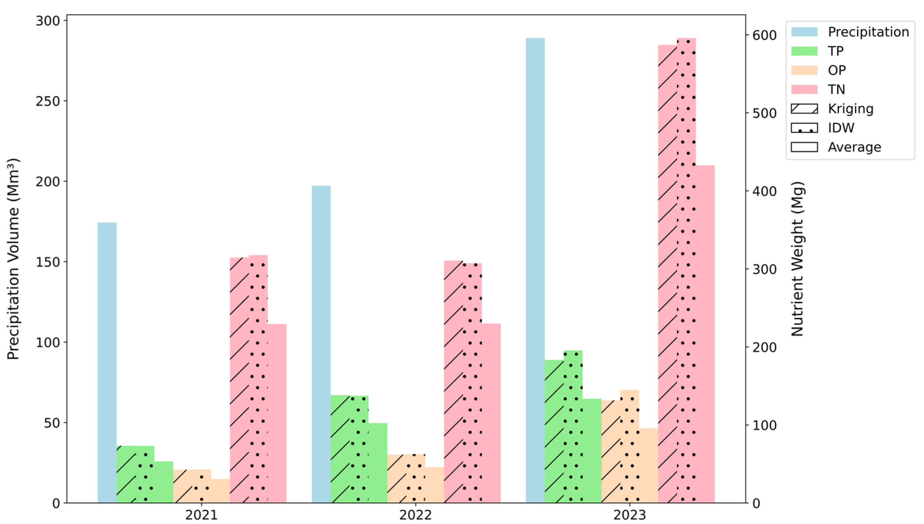
4.1. Annual Load Rates

Figure 10 shows the annual totals for precipitation (Mm³) and AD loads for TP, OP, and TN (in Mg or Metric tons). In 2021, the total precipitation volume was 174 Mm³, increasing to 197 Mm³ in 2022 and reaching 289 Mm³ in 2023 (Figure 10). The AD loads for all three nutrients follow the precipitation totals, which increase over the three-year period. The two spatial interpolation methods, Kriging and IDW, provide similar estimates, with IDW giving slightly higher estimates in 2023 than Kriging but almost identical estimates for 2021 and 2022. We also computed loads assuming the concentration over the Bay was the average of the concentration measured at the sites for a comparison. For all three years and all three nutrients, the estimate calculated using the average concentrations was significantly lower than the loads estimated using spatial interpolation. We will discuss the spatial distribution of the loads in more detail below.

Table 6. Annual AD loads for TP, OP, and TN over the three-year study period (2021, 2022, and 2023) estimated using three different spatial interpolation methods: Kriging, IDW, and the average values.

	2021			2022			2023
	Kriging (Mg)	IDW (Mg)	Avg (Mg)	Kriging (Mg)	IDW (Mg)	Avg (Mg)	Kriging (Mg)	IDW (Mg)	Avg (Mg)
TP	73.3	73.2	53.4	138.2	137.5	102.5	183.2	195.5	133.6
OP	42.6	42.8	31.0	62.0	62.6	45.9	131.6	145.0	95.8
TN	314.5	317.5	229.4	310.7	307.3	230.1	587.0	595.8	432.8

shows that the TP, OP, and TN loads follow similar trends, with Kriging-estimated TP annual loads of 73, 138, and 183 Mg and Kriging-estimated OP annual loads of 42, 62, and 131 Mg in 2021, 2022, and 2023, respectively (Figure 10 and Table 6). IDW-estimated values were similar, with TP load estimates of 73, 137, and 195 Mg and OP load estimates of 43, 62, and 145 Mg for 2021, 2022, and 2023, respectively (Figure 10 and Table 6). TN exhibited a different pattern, with Kriging-estimated TN loads of 314 Mg in 2021 and 311 Mg in 2022, which are about the same, but the estimated TN load in 2023 was significantly higher, at 587 Mg, almost double the load in the previous two years (Figure 10 and Table 6). The IDW-estimated loads were essentially the same as those estimated using Kriging (Table 6). The AD loads estimated using the average values were approximately 73% of those estimated using Kriging or IDW.

In Figure 1, we present the area we defined as Farmington Bay, based on statutes and geography, and further divided the Bay into Wetland and Lake areas. We based this division on the presence or absence of plant growth and open water. We chose to divide the Bay into two areas, and the impact of AD loads in these two areas may be different, though we have not explored this issue. AD loads in the lake area immediately impact the water column, raising water column nutrient concentrations. AD loads in the Wetland area are more complex and involve the interaction of plants, soil sorption, and potentially other processes.

Figure 11 shows the cumulative AD loads (Mg) separated by wetland and lake areas over the three-year study period. The left panel shows the cumulative loads for the lake area, and the right panel presents the cumulative loads for the wetland area. The areas are delineated in Figure 1. From top to bottom, the nutrients are arranged as follows: TP, OP, and TN. The graphs show that the loading rates are relatively constant and similar for both areas, with increases in late summer and fall following precipitation patterns. The total loads are different because of the difference in the size of the two areas.

Both the lake and wetland areas show a significant AD load for all three nutrients on 13 April 2023, which was caused by a very large amount of precipitation between the previous sample on 16 March and the 13 April 2023 sample. While there were several precipitation events during this period, we collected only one concentration sample on 13 April 2023. This single sample likely represented a conservative estimate of concentrations over these precipitation events, as the large rainfall events most likely resulted in dilution of the samples because the samplers overflowed. During this period, the precipitation measured at the seven stations ranged from 74 to 162 mm, with an average of 106.2 mm. This single event generated Kriging-estimated AD loads of 101, 89, and 231 Mg for TP, OP, and TN, respectively. The AD loads from this single load had an order of magnitude similar to that of the total annual loads.

As with the annual AD loads, the Kriging- and IDW-estimated cumulative AD loads are similar, though there is some difference in the estimated load from the 13 April 2023 event for OP, with the Kriging load being lower in the Lake area and higher in the Wetland area. This is a result of where the largest loading rates occurred.

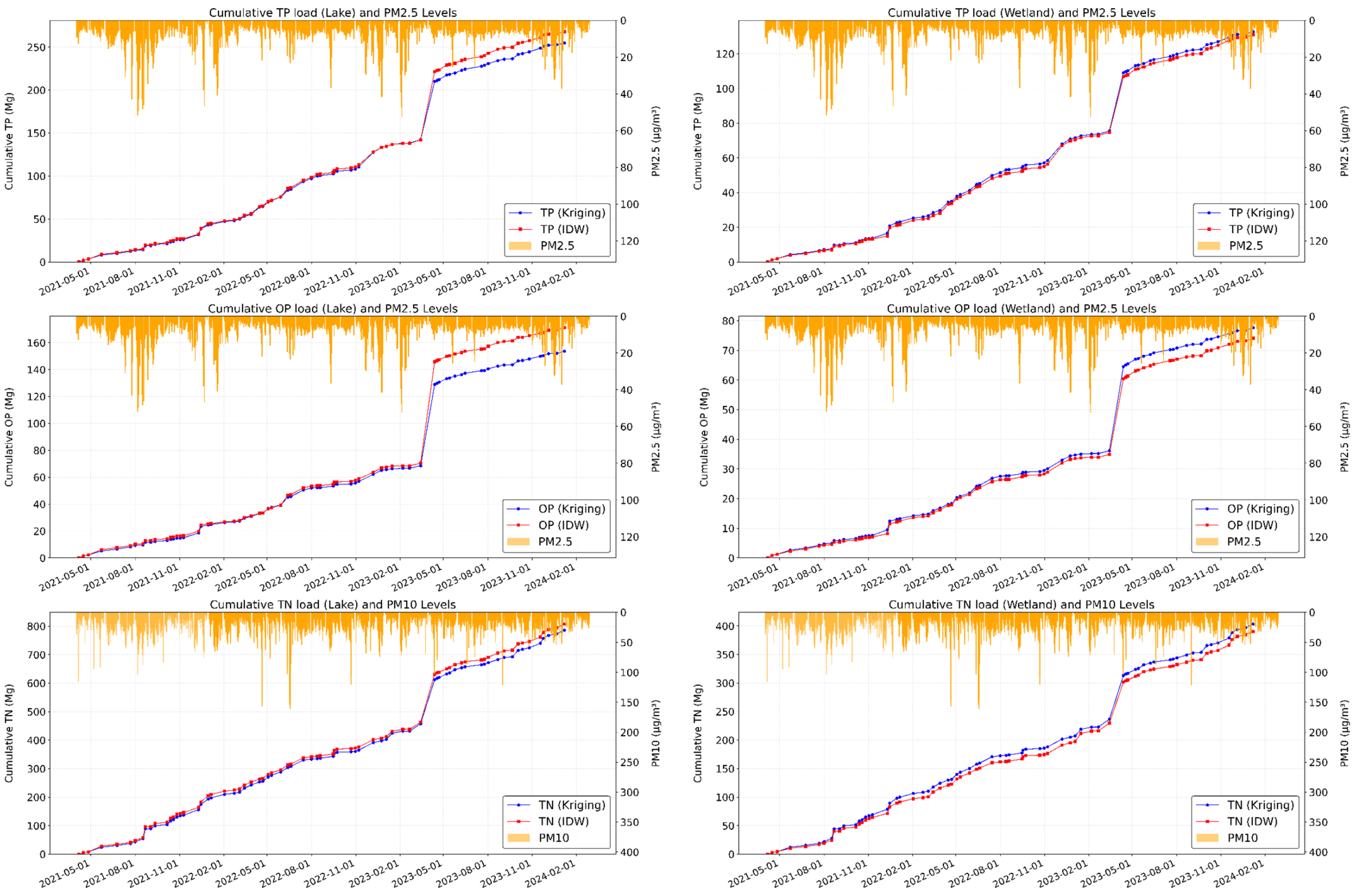
4.2. Nutrient Loads and Air Quality Analysis

Figure 11 shows the air pollutant levels of PM2.5 and PM10 measured in addition to the cumulative AD loads. We used PM10 data from an EPA air quality station located at 240 N 1950 W, Salt Lake City, and the PM2.5 data from Herriman EPA station. Herriman station is over 20 km south of the lake, but it is one of the closest stations with PM2.5 data. In Figure 11, the PM10 data are plotted in the bottom panel with the TN loads, while the PM2.5 data are plotted in the top two panels with the TP and OP data. We chose to present the data in this way as relatively coarser particles along with fine pollutants contribute to TN [31], while finer pollutants have greater percentages of phosphorus than coarser ones [32].

The atmospheric particulate data and AD loads were not strongly correlated. The one exception was during 2023, when we saw both high PM2.5 levels and PM10 levels along with increased nutrient deposits (TP, TN, and OP) coinciding with the large deposition event leading to the 13 April event. PM2.5 values were high immediately prior to this event. This increase, along with the heavy rainfall during this time, suggests that the combination of high levels of particulate matter and precipitation may have led to higher AD rates. However, the data imply that the large amount of precipitation was the main driver.

The lack of consistent relationships between pollution and AD levels suggests that nutrient deposits in Farmington Bay are influenced by various environmental factors, including coarse dust, not just fine particulate levels.

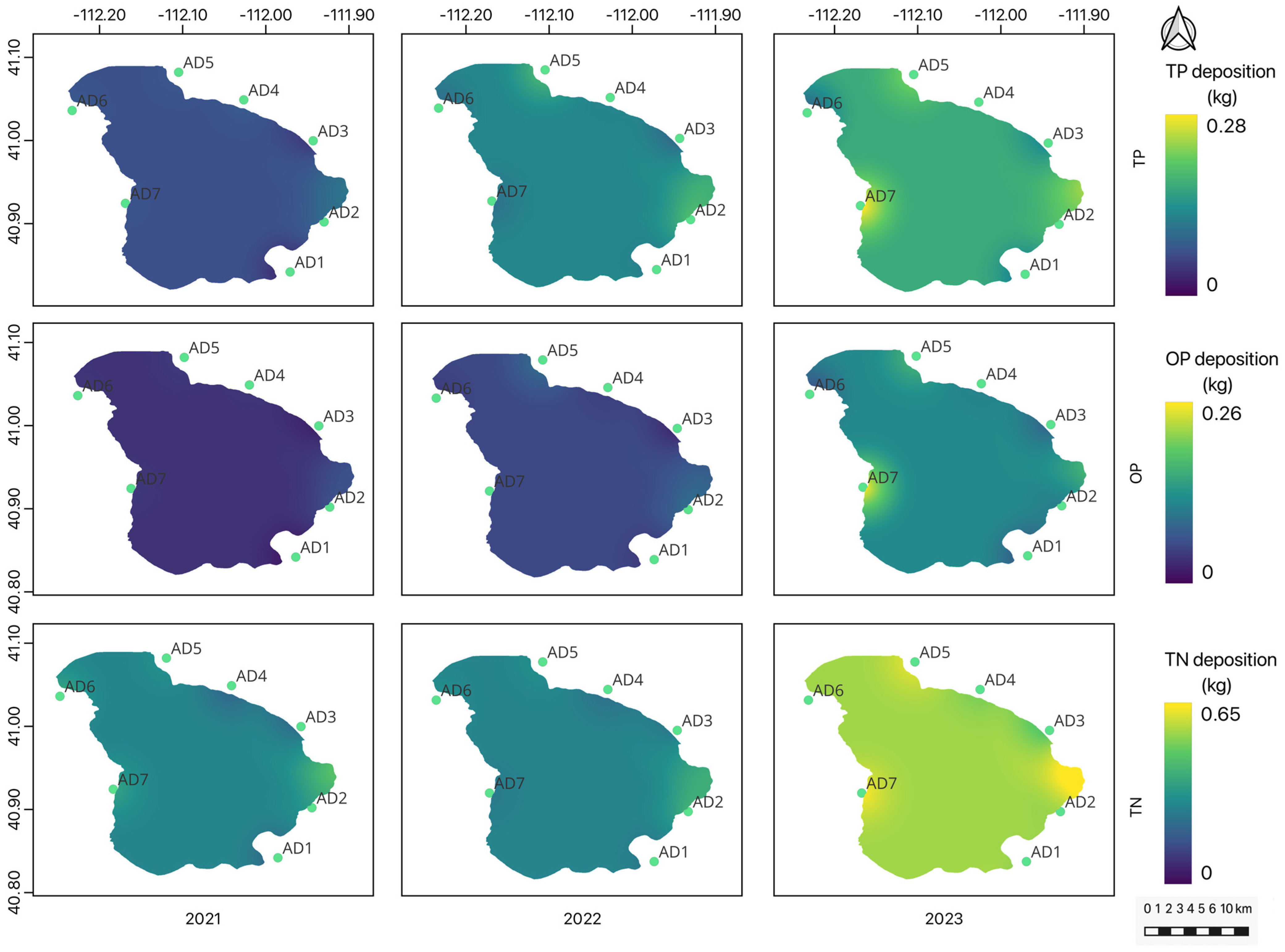
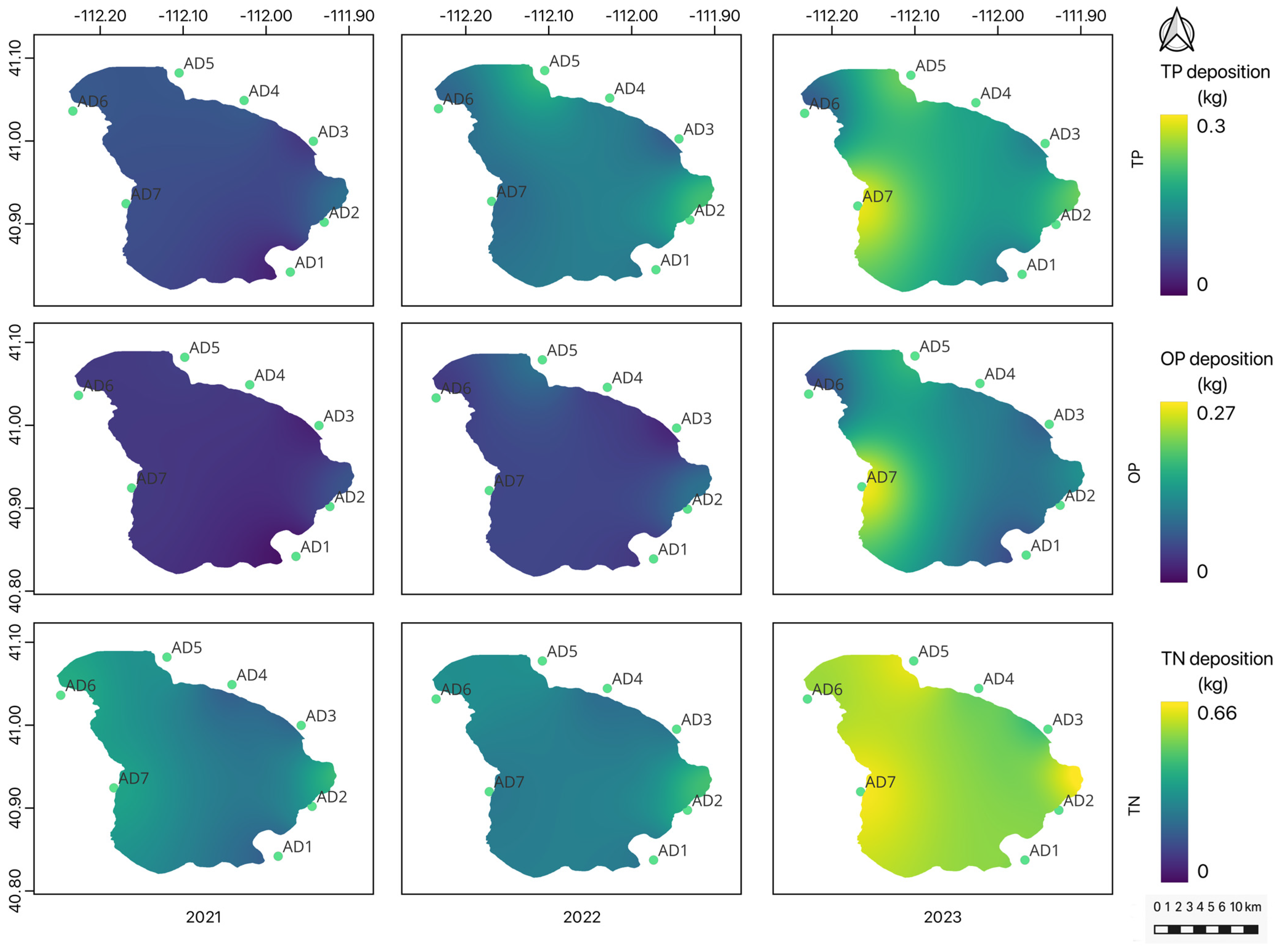
4.3. Spatial and Temporal Distribution of AD Loads

The spatial analysis of AD revealed distinct temporal and spatial patterns across Farmington Bay. Figure 12 presents the estimates made using Kriging spatial interpolation, while Figure 13 presents the IDW results. Both the Kriging and IDW estimates compute a mean value when there is a large distance from the stations. This can be seen in Figure 12, where the center of the Bay is essentially the mean value and is the same for both methods. This value is representative of the value used in the average method. The plots show that IDW has a larger correlation length than the range we used for Kriging, meaning that each individual station influences a larger region before returning to the average value. All nutrients exhibited increased loads from 2021 to 2023, with 2023 showing a peak load, largely driven by the April 2023 event. We used QGIS, version 3.4, to generate spatial figures (www.qgis.org/).

The central eastern region of Farmington Bay demonstrated consistently elevated nutrient deposition across all study years (AD2 and AD5), while the western sector, particularly near Buffalo Pens station (AD6), also maintained higher AD levels. The central eastern station, AD2, is near the urban areas and the Legacy Parkway. The northernmost station on the eastern side, AD5, is also higher than average and close to urban development. These patterns are best observed in Figure 13, though they are also apparent in Figure 12.

The northwestern area showed relatively higher concentrations throughout the study period. The TP and OP concentrations near Buffalo Pens station (AD6) remained comparable between 2021 and 2022, followed by a marked increase in 2023. The northeastern region experienced substantial increases in TP and OP deposition during the 2022–2023 period compared to the 2021 baseline levels. The eastern zone maintained consistently elevated AD levels for all nutrients throughout the study period. The interior portion of the lake is approximately the average value as this area is distant from any measurement station.

5. Discussion

5.1. Spatial and Temporal AD Load Variation

The Kriging and IDW spatial interpolation methods yielded very similar AD load estimates, while the loads estimated using the average of the measurements were about 70% lower. An analysis of the data grouped the seven stations into either two or three groups based on concentrations (Table 5). The stations with higher mean concentrations are not close to other stations, meaning that using either Kriging or IDW influences more than 1/7 the total area, while all the stations contribute 1/7 to the total when the average method is used.

The eastern side of the study region exhibited significantly higher atmospheric deposition (AD) rates. This spatial variation may be attributed to multiple factors, including prevailing wind patterns and potential limitations in sampling accessibility. The reduced sampling coverage on the western side, particularly in the Antelope Island area, could have introduced sampling bias that influenced the spatial distribution of nutrient deposition we observed.

In the study period, there was a significant increase in annual precipitation from 2021 to 2023, and there was a corresponding increase in AD nutrient loads. Because of the sampling method we used, i.e., collecting concentration data from precipitation samples and then computing nutrient loading mass based on the total precipitation volume over Farmington Bay, the precipitation and AD loads are somewhat correlated. During some storms, large precipitation events resulted in lower concentrations, probably due to dilution, while smaller events led to larger concentrations. These processes somewhat offset a direct correlation between precipitation and nutrient AD load.

Precipitation was the primary driver of AD nutrient loads, with the spatial distribution of nutrient concentration measurements also impacting total loads. Sampling stations near urban areas exhibited higher concentrations than other stations, though the southern station on Antelope Island, AD7, also had high concentrations. Nutrient concentrations were notably higher in areas adjacent to industrial and transportation zones within the study region, suggesting a significant anthropogenic influence on nutrient loading. The high concentrations measured on Antelope Island, specifically AD7 Garr Ranch, cannot be explained by industry or transportation. We did not explore this topic, but we expect this finding can be attributed to the higher dust levels in this area.

We arbitrarily divided Farmington Bay into lake and wetland areas derived from USGS flooded area. This is an arbitrary boundary, but we felt that nutrient loads atmospherically deposited in wetlands may have impacts different from those of loads deposited in open water.

Our definition of the Farmington Bay area is based on our interpretation of the corresponding statutory and regulatory definitions. However, the area of Farmington Bay used in this study is larger than that used in previous papers.

5.2. Relation to Previous Studies

We examined the influence of fine particulate matter in the atmosphere on loading events. Generally, there were no obvious correlations or patterns, except for the 13 April 2023 load, which was preceded by higher particulate concentrations. Data from Utah Lake, about 50 km south of Farmington Bay, reflected results obtained using different AD measurement methods. One study used the same methods used in this study, collecting precipitation, measuring nutrient concentration, and then computing loads using total precipitation [17]. The authors of a second set of studies used a wet collection method, where a container with a known area was exposed to the atmosphere with both concentration and volume measurements collected weekly [15,16]. From these data, a mass-per-area loading rate was computed for each week, with total loads based on the spatial interpolation of these measured rates.

Our measurement approach does not capture AD nutrient loads from fine particulate matter, which does not settle from the atmosphere [17]. However, these fine particles are captured when these particles contact a water surface. This means that nutrient loads in a water body are higher than those on a land surface.

Brown et al. [17] found that AD nutrient loads estimated via precipitation concentration were only 25% to 40% of loads based on measurements from samplers that captured settlement (dust), contact (small particles), and precipitation [16,17]. Based on these observations, the total AD nutrient loads in Farmington Bay could be 2 to 3 times higher than those estimated in this study. However, the Utah Lake study only considered loads deposited on the surface of the lake. This study includes significant areas that are not currently water surfaces, so the difference may not be as large.

6. Conclusions

We quantified AD loads in the Farmington Bay ecosystem using data collected over a 3-year period. We analyzed nutrient concentrations from 509 TP, 507 OP, and 511 TN samples collected across seven locations. We computed AD loads using two spatial interpolation methods, Kriging and IDW, and also estimated loads using the average concentration for a given sampling date. The estimated nutrient loads demonstrated significant variability, influenced by fluctuations in nutrient concentrations, precipitation patterns, and the spatial heterogeneity of measurements. Notably, the measured concentrations and precipitation amounts exhibited considerable temporal and spatial variations, with the measurements taken simultaneously revealing substantial differences across sampling locations. Comparative analysis of the two interpolation methods revealed distinct load estimations, with each method providing unique insights into the atmospheric nutrient deposition dynamics of the Farmington Bay ecosystem.

We estimated annual nutrient loads atmospherically deposited in Farmington Bay amount to between 306 and 594 Mg of TN, 73 and 195 Mg of TP, and 43 and 144 Mg of OP over the study period (Table 6). The loads in 2023 were significantly higher than the estimated loads in 2021 and 2022. This disparity was caused by the significantly higher precipitation in 2023 and a large single load, computed using the 13 April 2023 concentration sample, which contained a series of large precipitation events. The loads in 2021 and 2022 varied from 306 to 316 Mg for TN, 73 to 138 Mg for TP, and 43 to 62 Mg for OP (Table 6). The loads in 2023 were much higher, with approximately 590 Mg for TN, 190 Mg for TP, and 140 Mg for OP (Table 6).

Previous studies have shown that the AD nutrient loads from fine particulate matter may be significant, with the loads estimated using our sampling method being only 25% to 40% of those estimates made using methods that capture the total load including fine particulates [17]. This means that the total AD nutrient loads in Farmington Bay could be two to three times larger than our estimates. However, as the area of Farmington Bay includes areas that are not water surfaces, this difference may not be so great.

References

1. Bennett, M.G.; Schofield, K.A.; Lee, S.S.; Norton, S.B. Response of Chlorophyll a to Total Nitrogen and Total Phosphorus Concentrations in Lotic Ecosystems: A Systematic Review Protocol. Environ. Evid. 2017, 6, 18. [Google Scholar] [CrossRef] [PubMed]
2. Komala, P.S.; Primasari, B.; Ayunin, Q. The Influence of the Physicochemical Parameters on the Ortho Phosphate and Total Phosphate Concentrations of Maninjau Lake. J. Phys. Conf. Ser. 2020, 1625, 012061. [Google Scholar] [CrossRef]
3. Blaas, H.; Kroeze, C. Excessive Nitrogen and Phosphorus in European Rivers: 2000–2050. Ecol. Indic. 2016, 67, 328–337. [Google Scholar] [CrossRef]
4. Dabrowski, J.M. Applying SWAT to Predict Ortho-Phosphate Loads and Trophic Status in Four Reservoirs in the Upper Olifants Catchment, South Africa. Hydrol. Earth Syst. Sci. 2014, 18, 2629–2643. [Google Scholar] [CrossRef]
5. Hillery, B.R.; Simcik, M.F.; Basu, I.; Hoff, R.M.; Strachan, W.M.J.; Burniston, D.; Chan, C.H.; Brice, K.A.; Sweet, C.W.; Hites, R.A. Atmospheric Deposition of Toxic Pollutants to the Great Lakes As Measured by the Integrated Atmospheric Deposition Network. Environ. Sci. Technol. 1998, 32, 2216–2221. [Google Scholar] [CrossRef]
6. Koszelnik, P. Atmospheric Deposition as a Source of Nitrogen and Phosphorus Loads into the Rzeszów Reservoir, SE Poland. Environ. Prot. Eng. 2007, 33, 157. [Google Scholar]
7. Zheng, T.; Cao, H.; Liu, W.; Xu, J.; Yan, Y.; Lin, X.; Huang, J. Characteristics of Atmospheric Deposition during the Period of Algal Bloom Formation in Urban Water Bodies. Sustainability 2019, 11, 1703. [Google Scholar] [CrossRef]
8. Guieu, C.; Aumont, O.; Paytan, A.; Bopp, L.; Law, C.S.; Mahowald, N.; Achterberg, E.P.; Marañón, E.; Salihoglu, B.; Crise, A.; et al. The Significance of the Episodic Nature of Atmospheric Deposition to Low Nutrient Low Chlorophyll Regions. Glob. Biogeochem. Cycles 2014, 28, 1179–1198. [Google Scholar] [CrossRef]
9. Donaghay, P.L.; Liss, P.S.; Duce, R.A.; Kester, D.R.; Hanson, A.K. The Role of Episodic Atmospheric Nutrient Inputs in the Chemical and Biological Dynamics of Oceanic Ecosystems. Oceanography 2015, 4, 62–70. [Google Scholar] [CrossRef]
10. Loÿe-Pilot, M.D.; Martin, J.M. Saharan Dust Input to the Western Mediterranean: An Eleven Years Record in Corsica. In The Impact of Desert Dust Across the Mediterranean; Guerzoni, S., Chester, R., Eds.; Springer: Dordrecht, The Netherlands, 1996; pp. 191–199. ISBN 978-94-017-3354-0. [Google Scholar]
11. Guerzoni, S.; Chester, R.; Dulac, F.; Herut, B.; Loÿe-Pilot, M.-D.; Measures, C.; Migon, C.; Molinaroli, E.; Moulin, C.; Rossini, P.; et al. The Role of Atmospheric Deposition in the Biogeochemistry of the Mediterranean Sea. Prog. Oceanogr. 1999, 44, 147–190. [Google Scholar] [CrossRef]
12. Bonnet, S.; Guieu, C. Atmospheric Forcing on the Annual Iron Cycle in the Western Mediterranean Sea: A 1-Year Survey. J. Geophys. Res. Oceans 2006, 111, C09010. [Google Scholar] [CrossRef]
13. Guieu, C.; Dulac, F.; Desboeufs, K.; Wagener, T.; Pulido-Villena, E.; Grisoni, J.-M.; Louis, F.; Ridame, C.; Blain, S.; Brunet, C.; et al. Large Clean Mesocosms and Simulated Dust Deposition: A New Methodology to Investigate Responses of Marine Oligotrophic Ecosystems to Atmospheric Inputs. Biogeosciences 2010, 7, 2765–2784. [Google Scholar] [CrossRef]
14. Ternon, E.; Guieu, C.; Loÿe-Pilot, M.-D.; Leblond, N.; Bosc, E.; Gasser, B.; Miquel, J.-C.; Martín, J. The Impact of Saharan Dust on the Particulate Export in the Water Column of the North Western Mediterranean Sea. Biogeosciences 2010, 7, 809–826. [Google Scholar] [CrossRef]
15. Olsen, J.M.; Williams, G.P.; Miller, A.W.; Merritt, L. Measuring and Calculating Current Atmospheric Phosphorous and Nitrogen Loadings to Utah Lake Using Field Samples and Geostatistical Analysis. Hydrology 2018, 5, 45. [Google Scholar] [CrossRef]
16. Barrus, S.M.; Williams, G.P.; Miller, A.W.; Borup, M.B.; Merritt, L.B.; Richards, D.C.; Miller, T.G. Nutrient Atmospheric Deposition on Utah Lake: A Comparison of Sampling and Analytical Methods. Hydrology 2021, 8, 123. [Google Scholar] [CrossRef]
17. Brown, M.M.; Telfer, J.T.; Williams, G.P.; Miller, A.W.; Sowby, R.B.; Hales, R.C.; Tanner, K.B. Nutrient Loadings to Utah Lake from Precipitation-Related Atmospheric Deposition. Hydrology 2023, 10, 200. [Google Scholar] [CrossRef]
18. Gaichuk, I.V.; Finley, H. Groundwater Nutrient Fluxes and Hydrological Dynamics in the Farmington Bay Wetlands. Master’s Thesis, The University of Utah, Salt Lake City, UT, USA, 2023. [Google Scholar]
19. Gunnell, N.V. A Study of the Anthropogenic Impact in Farmington Bay through Isotopic and Elemental Analysis. Master’s Thesis, Brigham Young University, Provo, UT, USA, 2020. [Google Scholar]
20. Wurtsba, W.; Richards, C.; Hodson, J.; Rasmussen, C.; Winter, C. Biotic and Chemical Changes Along the Salinity Gradient in Farmington Bay, Great Salt Lake; Utah State University, Utah Division of Water Quality: Logan, UT, USA, 2015. [Google Scholar]
21. Wurtsbaugh, W.; Marcarelli, A. Eutrophication in Farmington Bay, Great Salt Lake, Utah 2005 Annual Report; Utah State University: Logan, UT, USA, 2005. [Google Scholar]
22. Armstrong, T.; Wurtsbaugh, W.A. Impacts of Eutrophication on Benthic Invertebrates & Fish Prey of Birds in Farmington and Bear River Bays of Great Salt Lake; Watershed Sciences Faculty Publications; Utah State University: Logan, UT, USA, 2019; p. 41. [Google Scholar]
23. Wurtsbaugh, W.; Marcarelli, A.M.; Christison, C.; Moore, J.; Gross, D.; Bates, S.; Kircher, S.J. Comparative Analysis of Pollution in Farmington Bay and the Great Salt Lake, Utah; Watershed Sciences Faculty Publications; Utah State University: Logan, UT, USA, 2002. [Google Scholar]
24. Peretti, M.; Piñeiro, G.; Fernández Long, M.E.; Carnelos, D.A. Influence of the Precipitation Interval on Wet Atmospheric Deposition. Atmos. Environ. 2020, 237, 117580. [Google Scholar] [CrossRef]
25. Stevenazzi, S.; Camera, C.A.S.; Masetti, M.; Azzoni, R.S.; Ferrari, E.S.; Tiepolo, M. Atmospheric Nitrogen Depositions in a Highly Human-Impacted Area. Water Air Soil Pollut. 2020, 231, 276. [Google Scholar] [CrossRef]
26. Tarboton, D.; Merck, M. Great Salt Lake Bathymetry, Hydroshare. 2023. Available online: http://www.hydroshare.org/resource/582060f00f6b443bb26e896426d9f62a (accessed on 10 November 2024).
27. Mitchell, L.E.; Zajchowski, C.A.B. The History of Air Quality in Utah: A Narrative Review. Sustainability 2022, 14, 9653. [Google Scholar] [CrossRef]
28. Hansen, J.C.; Woolwine, W.R., III.; Bates, B.L.; Clark, J.M.; Kuprov, R.Y.; Mukherjee, P.; Murray, J.A.; Simmons, M.A.; Waite, M.F.; Eatough, N.L.; et al. Semicontinuous PM2.5 and PM10 Mass and Composition Measurements in Lindon, Utah, during Winter 2007. J. Air Waste Manag. Assoc. 2010, 60, 346–355. [Google Scholar] [CrossRef]
29. Horel, J.D.; Powell, J.T. Analysis and Prediction of Summer Rainfall over Southwestern Utah. Weather Forecast. 2024, 39, 1007–1021. [Google Scholar] [CrossRef]
30. Sainani, K.L. Dealing with Non-Normal Data. PM&R 2012, 4, 1001–1005. [Google Scholar] [CrossRef]
31. Yu, X.; Wong, Y.K.; Yu, J.Z. Abundance and Sources of Organic Nitrogen in Fine (PM2.5) and Coarse (PM2.5–10) Particulate Matter in Urban Hong Kong. Sci. Total Environ. 2023, 901, 165880. [Google Scholar] [CrossRef] [PubMed]
32. Meng, Y.; Li, R.; Fu, H.; Bing, H.; Huang, K.; Wu, Y. The Sources and Atmospheric Pathway of Phosphorus to a High Alpine Forest in Eastern Tibetan Plateau, China. J. Geophys. Res. Atmos. 2020, 125, e2019JD031327. [Google Scholar] [CrossRef]
Figure 1. Farmington Bay areas (lake and wetland) along with the AD concentration, precipitation, and wind measurement stations. We divided Farmington Bay into a water area (blue) measuring 325 km2 and a wetland area (green) measuring 165 km2, making a total area of 490 km2.
Hydrology 12 00131 g001
Figure 2. A precipitation-AD-measuring station. The large funnel collects and directs rainwater to the collection tube below the funnel.
Hydrology 12 00131 g002
Figure 3. Distribution of daily precipitation data by station over the three-year study period. The ends of the boxes represent the 25th and 75th quartiles, while the ends of the whiskers represent the 1.5 interquartile range (IQR), with the line indicating the 50th quartile or median value.
Hydrology 12 00131 g003
Figure 4. Monthly distribution of daily precipitation across all stations over the three-year study period. The ends of the boxes represent the 25th and 75th quartiles, and the ends of the whiskers represent the 1.5 interquartile range (IQR), with the line indicating the 50th quartile or median value.
Hydrology 12 00131 g004
Figure 5. Wind roses based on 15 min wind data from 2021. The left panel includes all wind events, and the right panel only includes measurements over 10 miles per hour (mph) (4.5 m/s). The original data are in mph, and the figure reflects these units.
Hydrology 12 00131 g005
Figure 6. Distributions for the three nutrients. All are skewed right, with most values situated towards the low end of the range, but all exhibit significant tails with a few high values.
Hydrology 12 00131 g006
Figure 7. Correlation heat map for TN, OP, and TP nutrient concentration measurements.
Hydrology 12 00131 g007
Figure 8. Distribution of each nutrient at each location. TN has different scale (right) than TP and OP (left). The ends of the boxes represent the 25th and 75th quartiles, and the ends of the whiskers represent the 1.5 interquartile range (IQR), with the line indicating the 50th quartile or median value.
Hydrology 12 00131 g008
Figure 9. TP distributions by site. Boxes show the 25th, 50th, and 75th percentiles, with the diamonds and associated brackets showing the mean and 95% confidence interval. The whiskers represent 1.5 IQR, with outliers shown as circles.
Hydrology 12 00131 g009
Figure 10. Total annual values of precipitation volume and annual AD loads of TP, OP, and TN estimated using Kriging, IDW, and average values for the years 2021 to 2023 in Farmington Bay, for both lake and wetland areas combined.
Hydrology 12 00131 g010
Figure 11. Cumulative plots showing estimates from both Kriging and IDW interpolation methods for TP, OP, and TN in lake area (left) and wetland area (right) of Farmington Bay, with blue and red lines for Kriging and IDW, respectively. The plots include inverted bar graphs of particulate matter (PM) concentration levels. The bars show PM2.5 for TP and OP (top two panels) and PM10 for TN (bottom two panels). A large deposition event occurred on 13 April 2023, and it occurred at all the sampling sites, so we do not think it was a measurement mistake but instead an actual large loading event caused by a series of large precipitation events between the two samples.
Hydrology 12 00131 g011
Figure 12. Spatial analysis of annual AD patterns conducted using Kriging spatial estimation for TP, OP, and TN (top to bottom) across the Farmington Bay Area, Utah, for 2021, 2022, and 2023 in the left, center, and right columns, respectively. The data are given in Kg/grid-cell and indicate which areas of the Bay received most of the loads. Loads in 2023 were significantly higher than those in previous years, with about 1/3 of the total stemming from the 13 April 2023 load. The color scales for TP and OP are the same, with a different scale for TN, as the loads are larger.
Hydrology 12 00131 g012
Figure 13. Spatial analysis of annual AD patterns using IDW spatial interpolation for TP, OP, and TN (top to bottom) across the Farmington Bay Area, Utah, for 2021, 2022, and 2023 in the left, center, and right columns, respectively. The data are given in Kg/grid-cell and indicate which areas of the Bay received most of the loads. Loads in 2023 were significantly higher than those in previous years, mostly driven by the 13 April load.
Hydrology 12 00131 g013