Seasonal Freshwater Inflows in Cochin Backwater Estuary Inferred from Stable Isotopes and Machine Learning

Abstract

The Cochin Backwater region in Southern India is one of the most dynamic estuaries, strongly influenced by seasonal river runoff and seawater intrusion. This study explores the relationship between monsoonal rains, salinity, and stable isotopic composition (δ¹⁸O and δ¹³C) to estimate the contribution of freshwater fluxes at different seasonal intervals for the Cochin Backwater (CBW) estuary. Seasonal variations in oxygen isotopes and salinity revealed distinct trends indicative of freshwater–seawater mixing dynamics. The comparison of Local and Global Meteoric Water Lines highlighted the occurrence of enriched isotope values during the Premonsoon season, showing significant evaporation effects. Carbon (C) isotopic analysis in dissolved inorganic matter (δ¹³C_DIC) at 17 stations during the Premonsoon season revealed spatially distinct carbon dynamics zones, influenced by various sources. These characteristic zones were categorized as Zone 1, dominated by seawater, exhibiting heavier δ¹³C_DIC values; Zone 2, showing significant contributions of lighter terrestrial δ¹³C; and Zone 3, reflecting inputs from regional and local paddy fields with a distinct C₃ isotopic signature (−25‰), modified by estuarine productivity. In addition, different advanced machine learning techniques were tested to improve analysis and prediction of seasonal variations in isotopic composition and salinity. Although the data were sufficiently robust for demonstrating the feasibility and advantages of ML in isotopic hydrology, further expansion of the dataset would be essential for improving the accuracy of models, especially for δ¹³C. The combination of these advanced machine learning models not only improved the predictive accuracy of seasonal freshwater fluxes but also provided a robust framework for understanding the estuarine ecosystem and could pave the way for better management and conservation strategies of the CBW estuarine system.

1. Introduction

Estuaries are among the most dynamic transitional environments, acting as vital interfaces between terrestrial and marine systems. They provide a range of ecosystem services such as nutrient cycling, carbon sequestration, fisheries support, and biodiversity maintenance, making them critical socioecological systems worldwide [1]. The hydrology of estuaries is strongly governed by freshwater influx from rivers and saline water intrusion from the sea, processes that vary seasonally and exert profound influences on productivity, biogeochemistry, and ecological functioning. Globally, estuarine systems such as the Mekong Delta in Southeast Asia, the Amazon Estuary in South America, and Chesapeake Bay in North America have demonstrated how freshwater fluxes, tidal regimes, and anthropogenic pressures shape estuarine dynamics across spatial and temporal scales [1,2,3]. Understanding these dynamics is essential not only for local resource management but also for assessing the resilience of estuarine systems to climate variability and human-induced stressors.

In the Indian context, monsoon-fed estuaries represent a unique class of semi-enclosed coastal systems. Their hydrography is primarily regulated by the seasonal monsoons, in contrast to temperate estuaries where glacial meltwater or snowmelt often dominates seasonal fluxes [1,4]. Among these, the Cochin Backwater (CBW) estuary is one of the largest and most studied estuarine systems in Southern India. Fed by six rivers and strongly influenced by semi-diurnal tides, the CBW estuary experiences pronounced salinity stratification, seasonal freshwater inflows, and extensive anthropogenic interventions, including urbanization, dredging, and agricultural activities [5,6,7,8]. Prior studies in this estuary have largely focused on hydrochemistry, nutrient cycling, and anthropogenic impacts [6,7,8,9], yet a comprehensive seasonal assessment of freshwater fluxes using isotopic tracers has remained limited.

The primary sources of seasonal freshwater inflows into the CBW estuary are predominantly attributed to river discharges, as well as precipitation influenced by monsoonal patterns. CBW receives freshwater from six rivers, with the Periyar River contributing approximately 33% of the total river discharge (~19,000 million cubic meters/year) [10]. This riverine input is crucial for maintaining the estuarine salinity and nutrient levels, especially during the monsoon season when freshwater influx is at its peak [11]. In addition, these inflows significantly affect the estuarine ecosystem, nutrient dynamics, and isotopic signatures of the water. Seasonal variations in stable water isotopes indicate that monsoonal precipitation plays a significant role in freshwater inflow. The Southwest Monsoon (June–September) is characterized by marine moisture sources, while the Northeast Monsoon (October–December) shows continental contributions [12]. The isotopic composition of precipitation varies across different regions, reflecting the influence of altitude and local climatic conditions on freshwater sources [12].

Stable isotopes of oxygen (δ¹⁸O, δD) and carbon (δ¹³C) have long been recognized as robust tools to trace water sources, quantify mixing processes, and assess biogeochemical cycling in estuarine and coastal systems [13,14,15,16,17]. Globally, these approaches have successfully resolved freshwater–seawater mixing (e.g., Amazon, Mekong, Hooghly estuaries), evaporation effects, and carbon cycling linked to terrestrial versus marine inputs. In India, isotopic studies have addressed aspects of estuarine mixing in the Hooghly and Mandovi–Zuari estuaries [13,18] and carbon cycling in CBW [15,19], but these efforts have generally been localized in scope, event-specific, or limited to a single tracer. Systematic integration of δ¹⁸O, δD, and δ¹³C signatures with salinity to quantify freshwater contributions across multiple monsoon seasons remains underdeveloped, despite its potential to reveal spatial zonation and ecosystem-level processes.

Machine learning (ML) techniques are emerging as powerful alternatives to conventional statistical or box-model approaches in hydrology and geochemistry. Methods such as Artificial Neural Networks (ANNs), Random Forests (RFs), Support Vector Machines (SVMs), Gradient Boosting Machines (GBMs), and Gaussian Process Regression (GPR) have been widely applied to predict water quality parameters, isotopic compositions, and ecosystem responses in temperate and subtropical settings [20,21,22,23,24,25,26,27]. For example, in the Mediterranean Sea, RF and ANN models have successfully predicted isotopic and salinity variations with high accuracy [20]. Similarly, ML-based approaches have been used to forecast groundwater isotopes [21,24], eutrophication [23], and evaporation rates [26]. However, applications of ML in the Asian monsoon region, especially from an estuarine context are almost non-existent. To date, no study has systematically tested ML models for predicting stable isotopic tracers (δ¹⁸O, δ¹³C) and freshwater fluxes in tropical estuaries where seasonal variability is extreme.

Stable isotopic signatures, such as δ²H and δ¹⁸O, provide valuable insights into hydrological processes, including evaporation, precipitation, and mixing in complex tidal environments. The integration of ML models with isotopic data can enhance the accuracy of predictions by capturing the dynamic interactions within estuarine systems. Various ML models, including RF and Multivariate Adaptive Regression Spline (MARS), have been effectively used to reconstruct hydrological data, outperforming traditional methods like stage-discharge rating curves. These models have demonstrated reduced errors in predicting discharge, indicating their potential applicability in estuarine environments [28]. The use of stable isotopes in conjunction with machine learning can further refine predictions by providing continuous, high-resolution data on water residence times and mixing processes, which are critical for accurate inflow predictions [29]. While machine learning models and isotopic data offer promising tools for predicting freshwater inflows, challenges remain in accurately capturing the complex interactions in estuarine systems. Factors such as tidal influences, anthropogenic changes, and climatic variability can introduce uncertainties that require further refinement of models and methodologies. Nonetheless, the integration of these advanced techniques holds significant potential for enhancing our understanding and management of estuarine water resources.

In the above context, the present study provides the first combined application of stable isotopes and multiple machine learning models to estimate seasonal freshwater fluxes in the CBW estuary. The novelty of our work lies in comprehensive seasonal assessment to quantify freshwater contributions to CBW across Northeast Monsoon, Southwest Monsoon, and Premonsoon periods, using δ¹⁸O–salinity mass balance complemented by δ¹³C-based carbon cycling analysis. We used existing data from the Arabian Sea to establish seawater δ¹⁸O and salinity baselines and adopted seasonal rainwater composition from previous studies [30,31] for understanding the stable isotope mixing patterns. Furthermore, isotopic zonation of estuarine dynamics was studied using spatial field sampling to understand the effects of seawater dominance, terrestrial inputs, and agricultural runoff, with the aim of providing new insights into the biogeochemical stratification of the CBW estuary. In addition, with the aim of integrating ML techniques with isotope hydrology, we rigorously evaluated eight ML algorithms (RF, KNN, SVM, GBM, CART, GPR, ELM, RBNN) for predicting δ¹⁸O, δ¹³C, and salinity in the estuary. This is the first study in the Indian monsoon estuarine setting to systematically benchmark ML performance against isotope–salinity datasets. By doing so, this study not only addresses a critical knowledge gap in the estuarine isotope hydrology of the Indian subcontinent but also contributes a methodological advancement by coupling high-resolution geochemical tracers with state-of-the-art data-driven ML modeling approaches.

2. Materials and Methods

2.1. Study Area

Based on its dimensions, CBW is the largest estuarine system along the west coast of India and belongs to the Vembanad-Kol wetland system, one of the three Ramsar sites in Kerala that extends from Munambam (10°10′00″ N, 76°10′15″ E) in the north to Alappuzha (9°30′00″ N, 76°28′10″ E) in the south totalling 96.5 km in length (Figure 1). The width varies from 450 m to 4 km, and the depth ranges from 15 m at the Cochin Inlet to 3 m near the head, with an average depth of 1.5 m. The barrier spits are interrupted by tidal inlets at two locations: (i) Munambam Inlet in the north and (ii) Cochin Inlet in the middle.

The present study was conducted on CBW and Vembanad Lake, situated at the southern tip of the Indian subcontinent. This region experiences three distinct seasons: Premonsoon (PM, April–May), Southwest Monsoon (SWM, June–September), and Northeast Monsoon (NEM, October–December). During the monsoon season, the influx of freshwater significantly increases due to heavy precipitation, while the non-monsoon season (January–March) is characterized by reduced riverine input and dominant tidal forcing, leading to higher salinity levels in the estuary [14,32]. Water samples for δ¹⁸O and salinity analysis were collected fortnightly during high and low tides for a 1-year period between October and September of the subsequent year (

Table 1. Measured salinity and oxygen isotopic composition of Cochin Backwater collected biweekly during both low and high tides at sample site 1 as indicated in Figure 1.

Date of Sample Collection	Seasons	δ18OVSMOW (‰)		Salinity
		High Tide	Low Tide	High Tide	Low Tide
4-October	Northeast Monsoon	−2.84		0.2
18-October		−1.87	−1.9	8.5	5.1
2-November		−1.19	−3.49	12.6	11.1
16-November		−4.69	−4.21	1.9	1.3
2-December		−2.44	−3	11.5	7.1
16-December		−1.15	−2.22	19.4	12.3
31-December		−1.15	−1.54	20	16.2
15-January		−0.96	−1.86	19.6	17.8
30-January		−1.23	−0.7	21.1	18
13-February	Premonsoon	−0.41	−0.74	21.7	17.1
28-February		−0.3	−1.24	20.5	18.6
15-March		−0.58	−0.78	18.5	18.1
15-April		−0.75	−1.1	20.5	16.6
14-May		−0.72	−0.47	21.6	20.3
27-May		−1.01	−1.09	7.8	4.9
14-June	Southwest Monsoon	−3.72	−3.69	0.2	0.1
27-June		−3.2	−3.29	0.2	0.2
11-July		−2.83	−2.68	1	2.6
26-July		−2.66	−2.58	2.5	0.5
11-August		−2.26	−2.2	2.8	4
26-August		−2.74	−2.58	0.7	0.7
8-September		−2.01	−2.42	10.2	2.9
25-September		−5.01		0.1

). Fortnightly sampling during both high and low tides over a full annual cycle was essential to capture the temporal variability driven by monsoonal rainfall, tidal influences, and seasonal freshwater influx. This approach ensured high-resolution data reflecting both short-term tidal fluctuations and long-term seasonal shifts, which are critical for accurately characterizing estuarine mixing dynamics and validating isotope–salinity relationships. Additionally, a spatial survey covering 17 sites (Figure 1,

Table 2. Hydrological parameters of Cochin Backwater collected during the Premonsoon season.

Sl. No	Location	Lat (oN)	Long (oE)	Salinity (PSU)	δ18O (‰ VSMOW)	δ13CDIC (‰ VPDB)
1	Thevara ferry	9.926	76.304	0.10	0.42	−5.60
2	Panangad	9.883	76.331	18.80	0.54	−5.64
3	Arror	9.882	76.307	17.60	0.89	−10.52
4	Kudapuram (Eramallor)	9.829	76.320	15.70	NA	−9.01
5	Kodamthuruthu (Kuthiathodu)	9.803	76.326	13.10	2.49	−9.60
6	Thykkatusherry	9.773	76.331	11.70	3.31	−11.10
7A	Vyalar	9.718	76.345	10.40	1.52	−9.62
7B	Vyalar	9.718	76.350	10.40	0.43	−8.58
8	Punnamada	9.508	76.353	2.10	0.50	−14.09
9	Aaryad	9.544	76.353	0.10	1.76	−17.23
10	Pallathuserry	9.563	76.356	0.10	0.53	−21.34
11	Muhamma	9.604	76.362	3.40	1.23	−17.03
12	Thalayazham (Puthanpalam)	9.692	76.413	10.40	2.00	−11.97
13	Vaikom	9.749	76.389	11.60	3.06	−9.33
14	Kulasekaramagalam (Mekara)	9.799	76.379	11.90	0.78	−8.04
15	Punnakkaveli (South Paravoor)	9.855	76.379	12.45	2.45	−7.74
16	Chavakakadavuamera (Udayamperoor)	9.894	76.363	16.40	1.59	−7.20
17	Fort Kochi	9.968	76.244	28.00	−1.75	−2.90

) was conducted in the Premonsoon period (March–May) to document variability in isotopic composition and salinity. This spatial survey was conducted only in the Premonsoon period to capture the peak influence of seawater intrusion and evaporation-driven enrichment, which are most pronounced during the Premonsoon period when freshwater inflow is minimal. Documenting isotopic and salinity variability during this time provides critical insights into baseline estuarine dynamics before the onset of monsoonal dilution.

2.2. Sample Collection and Analysis

Surface water samples were collected in 50 mL HDPE bottles at a depth of 15 cm from the surface to avoid immediate surface film contaminants and stored until analysis. Sampling was conducted from the middle of the channel at each location to avoid bank effects. For the temporal study (Table 1), samples were collected fortnightly between the years 2009 and 2010 for one full year, at a single key station (Cochin Inlet, Station 1) during both high and low tides to capture the full range of tidal and seasonal variability at a strategic point of maximum seawater exchange. In total, 44 water samples were collected as shown in Table 1. For the spatial survey (Table 2), samples were collected from 17 stations/sampling points along the main axis of the estuary. It is important to note that this comprehensive spatial survey was conducted only during the Premonsoon period (March–May of 2015 for one year only). This period was specifically chosen to capture the baseline conditions of maximum seawater intrusion and salinity stratification before the onset of heavy monsoonal runoff. While this design provides a detailed spatial ‘snapshot’ under specific conditions, we acknowledge that it limits our ability to make direct spatial comparisons across all seasons, and that will be the focus of the future work.

Measurements of δ¹⁸O were conducted using the CO₂-H₂O equilibration method [33,34] on a Thermo Fisher MAT-253 isotope ratio mass spectrometer coupled with a GasBench II peripheral in a continuous flow mode, with a measurement reproducibility of 0.08‰. δD measurements were also carried out on the water samples with an aim to understand the dual water isotope behavior at the CBW estuary and compare with the well-established Meteoric Water Lines of the region. For δD analyses, samples were flushed with a He + H₂ (2.5%) mixture and equilibrated for 70 min at 25 °C in the presence of catalytic platinum sticks. The obtained reproducibility using this method was 1.2‰. Water samples were analyzed immediately after collection using a conductivity probe (Orion, range 0.1 to 42, accuracy ±0.1) connected to a Thermo Scientific (Bremen, Germany) Orion 5-star multimeter. The conductivity probe was standardized with Orion conductivity standards (147 μS/cm, 1413 μS/cm, and 12.9 mS/cm). For δ¹³C_DIC, water samples were collected in glass amber bottles with butyl rubber septa, treated with 1 mL of saturated HgCl₂ solution to inhibit biological activity, and stored. δ¹³C_DIC was measured by acidifying 2 mL of water with 0.5 mL of 100% orthophosphoric acid [35]. Standards, including NBS19 and MARJ1, were analyzed for calibration with a standard deviation of 0.09‰ for δ¹³C [36]. Rainfall data were obtained from the nearest weather station on Willingdon Island (latitude 9°57′14″ N, longitude 76°16′06″ E) (http://www.tutiempo.net, accessed on 12 June 2025) for comparison.

2.3. ML Methodology

To model and predict isotopic compositions and salinity, a suite of eight machine learning models was strategically selected to cover a range of learning approaches, from conventional algorithms to more advanced techniques. The rationale for this multimodel approach was to conduct a robust comparative analysis across diverse algorithmic families to assess their feasibility for this specific application. Given the relatively limited size of our dataset, we deliberately prioritized models that are less prone to overfitting and do not require extensive training data. Therefore, highly parameterized models such as Artificial Neural Networks (ANNs), which carry a greater risk of overfitting with smaller datasets, were excluded from this analysis in favor of a broader suite of benchmark and ensemble techniques. The selected models were chosen to represent a wide spectrum of learning strategies and are listed below:

• Conventional Models: K-Nearest Neighbor (KNN), Random Forest (RF), and Sup-port Vector Machine (SVM) were chosen as they have been previously applied in stable isotope modeling studies and serve as established benchmarks [20].
• Advanced Tree-Based Models: Gradient Boosting Machine (GBM) and Classification and Regression Tree (CART) were selected for their ability to capture complex non-linear interactions and provide insights into feature importance, which is crucial for understanding the environmental drivers.
• Other Advanced Models: Gaussian Process Regression (GPR) was included for its strength in quantifying prediction uncertainty. Extreme Learning Machines (ELMs) and Radial Basis Function Networks (RBNNs) were tested for their efficiency and effectiveness in modeling spatial gradients and patterns with potentially limited data.

The foundation of our predictive modeling workflow was the careful curation and preprocessing of the dataset. We selected four key predictor variables—latitude, longitude, month, and tide phase—as proxies for the spatial and temporal drivers of estuarine dynamics. These features were used to predict three target variables: salinity, δ¹⁸O, and δ¹³C. Prior to model training, a rigorous preprocessing pipeline was implemented to handle the diverse nature of this data. Continuous variables were normalized using Min–Max scaling to prevent features with larger numeric ranges from disproportionately influencing model outcomes. Categorical data, such as the tide phase, were numerically encoded to be machine-readable. Furthermore, the single missing data point for δ¹⁸O was addressed using Gaussian Process Regression, a method chosen for its ability to leverage the strong underlying correlation with salinity. For complete methodological transparency and to facilitate the replication of our results, all variables, their roles, and these specific preprocessing steps are consolidated and detailed in

Table 3. Description and preprocessing of features for machine learning models.

Feature Name	Role	Type	Unit/Description	Preprocessing Steps
Latitude	Predictor	Continuous	Degrees North (°N)	Normalized to a range using Min–Max scaling
Longitude	Predictor	Continuous	Degrees East (°E)	Normalized to a range using Min–Max scaling
Month	Predictor	Continuous	Numerical representation of the month (1 = January, …, 12 = December).	Normalized to a range using Min–Max scaling
Tide Phase	Predictor	Categorical	The tidal state during sampling (‘High Tide’ or ‘Low Tide’).	Converted to a binary numerical format: High Tide = 1, Low Tide = 0
Salinity	Target	Continuous	Practical Salinity Units (PSU)	Normalized to a range using Min–Max scaling
δ18O	Target	Continuous	Isotopic ratio relative to Vienna Standard Mean Ocean Water (‰ VSMOW).	Normalized to a range using Min–Max scaling. The single missing value from the spatial dataset was imputed via Gaussian Process Regression, using salinity as a covariance kernel
δ13C	Target	Continuous	Isotopic ratio relative to Vienna Pee Dee Belemnite (‰ VPDB).	Normalized to a range using Min–Max scaling

.

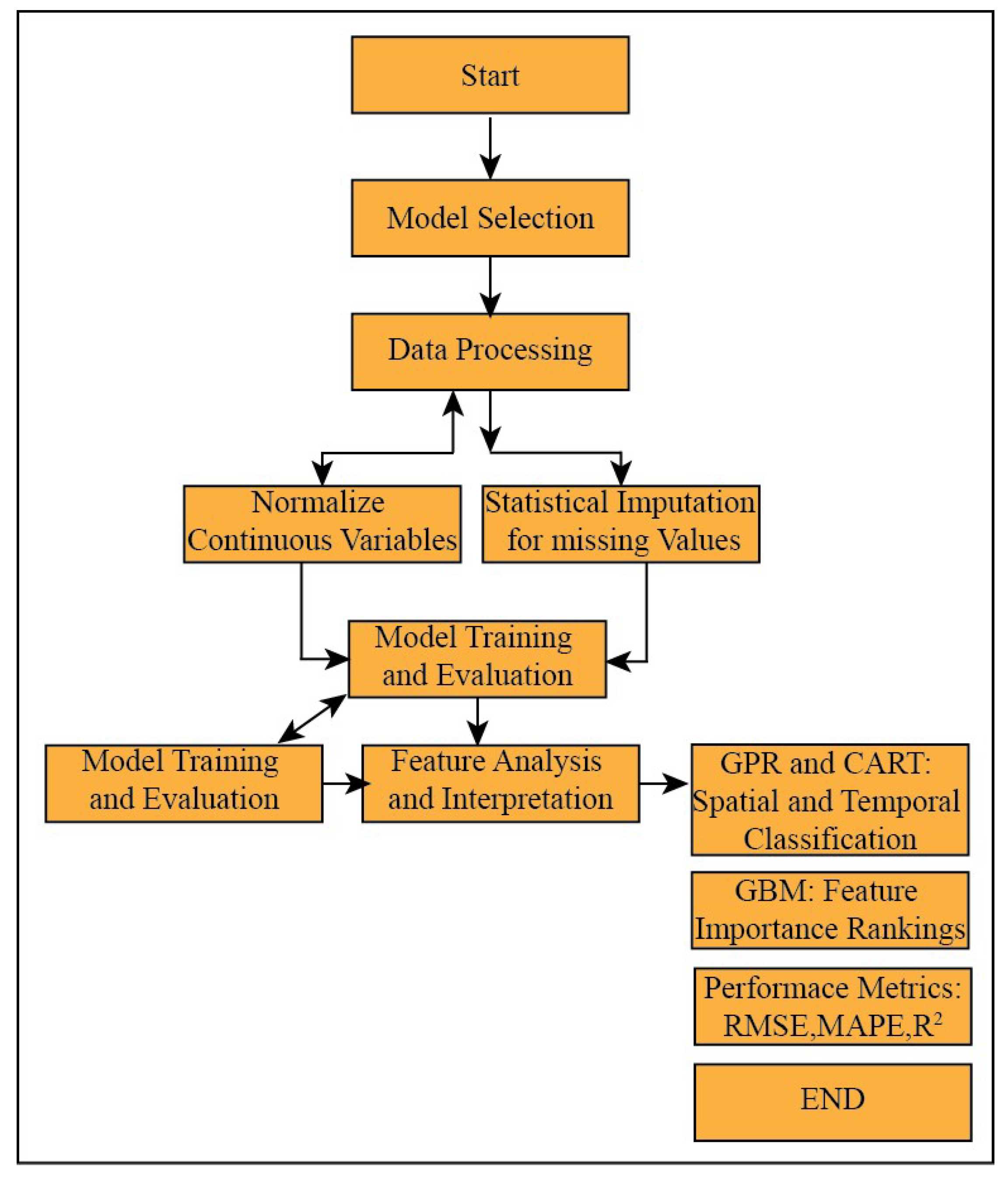
The overall workflow is depicted in Figure 2 and Table 3. The input features selected for the models included temporal variables (e.g., month, tidal phase) and spatial variables (latitude, longitude), which serve as proxies for the underlying environmental gradients. Before training, missing values for δ¹⁸O in the spatial dataset (one station) were imputed using Gaussian Process Regression, leveraging the strong covariance observed between salinity and δ¹⁸O. All continuous variables were normalized to a common scale to ensure compatibility across models. The dataset was partitioned into training (60%), validation (20%), and test (20%) subsets. Model hyperparameters were tuned using a Bayesian optimization approach over 100 iterations with the objective of minimizing the Root Mean Square Error (RMSE). Robustness was ensured through k-fold cross-validation during the training process.

The data preprocessing comprised all continuous variables, including salinity and isotopic ratios. All the data were normalized to ensure compatibility across models, and the missing values were addressed using statistical imputation methods. Hyperparameters were tuned via Bayesian optimization (GPyOpt library) with 100 iterations, prioritizing minimization of hydrological prediction uncertainty. A tiered data imputation of δ¹⁸O values (Table 2) was reconstructed via Gaussian Process Regression using salinity-δ¹⁸O covariance kernels. The Model Training and Evaluation step included dividing the data into training (60%), validation (20%), and test (20%) subsets. K-fold cross-validation was employed to ensure robust model evaluation. The determination of performance metrics included Root Mean Square Error (RMSE) (Equation (1)), Mean Absolute Percentage Error (MAPE) (Equation (2)), and Coefficient of Determination (R²) (Equation (3)) measures. The equations used for the individual performance metric estimations are as below:

$$RMSE=\sqrt{{\displaystyle \frac{1}{n}}{\sum }_{i=1}^n{\left(\widehat{y_i}-y_i\right)}^2}$$

(1)

$$MAPE={\displaystyle \frac{1}{n}}{\sum }_{i=1}^n|\widehat{y_i}-y_i|$$

(2)

$$R^2=1-{\displaystyle \frac{\sum {\left(y_i-\widehat{y_i}\right)}^2}{\sum {\left(y_i-\overline{y}\right)}^2}}$$

(3)

where n is the total number of observation data points, yᵢ is the observed (measured) value for the i-th data point, ŷᵢ is the predicted value for the i-th data point generated by the model, ȳ is the mean of the observed values, (ŷᵢ − yᵢ)² is the squared error between the predicted and observed values, and |ŷᵢ − yᵢ| is the absolute error between the predicted and observed values.

Feature analysis and interpretation was performed using GBM that provided feature importance rankings to identify key drivers of isotopic and salinity variations. GPR and CART enabled spatial and temporal classification of estuarine zones, revealing insights into monsoonal and non-monsoonal dynamics.

3. Results

3.1. Seasonal Variations in δ¹⁸O and Salinity

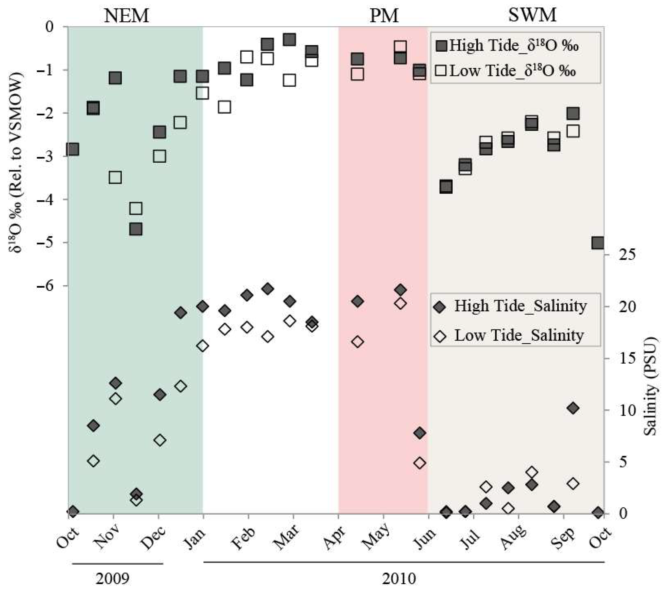
The seasonal δ¹⁸O and salinity data revealed significant oscillations in δ¹⁸O and salinity values, irrespective of tidal phases, as shown in Figure 3. During the Northeast Monsoon (NEM) period (October–December), δ¹⁸O values ranged from −4.69‰ to −1.15‰, with salinity values between 20 and 0.2. The Premonsoon (April–May) period exhibited δ¹⁸O values from −1.1‰ to −0.47‰, with corresponding salinity values from 21.6 to 4.9. In the Southwest Monsoon (SWM; gray region—Figure 3), δ¹⁸O reached its lowest value of −5‰ during high tide. The positive correlation between δ¹⁸O and salinity was evident across all seasons (Figure 3).

3.2. Spatial Variations in δ¹⁸O, δ¹³C, and Salinity

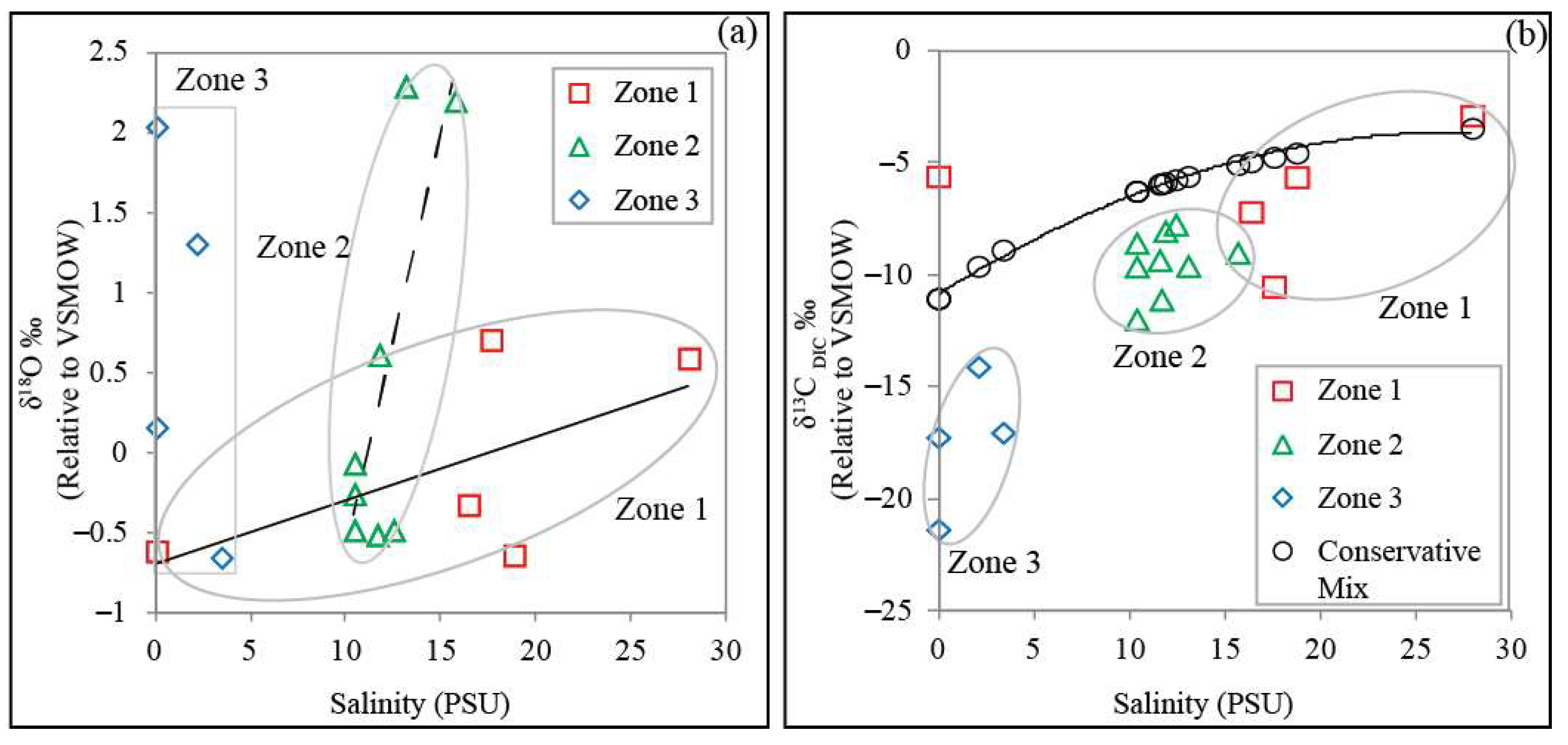
Spatial variations were pronounced, with δ¹⁸O values ranging from −1.75‰ to 3.31‰, and salinity values spanning from 0.1 to 28.0 across different stations (Table 2). Salinity and oxygen isotopic values varied significantly across the studied area, and three distinct spatial zones were evident. These were classified into Zone 1 (influenced by the Periyar River), with salinity ranging from 0.1 to 28.0, δ¹⁸O ranging between 0.7‰ and −0.6‰, and δ¹³C ranging from −2.9‰ to −10.5‰ (Figure 4); Zone 2 (influenced by other freshwater sources), with salinity ranging from 10.3 to 15.7, δ¹⁸O ranging from 2.2‰ to −0.5‰, and δ¹³C ranging from −7.7‰ to −11.9‰; and Zone 3 (Vembanad Lake), with salinity ranging from 0.1 to 3.4, δ¹⁸O ranging from 2.0‰ to −0.7‰, and δ¹³C ranging from −14.1‰ to −21.3‰ (Figure 4 and Table 2). The zones were classified following previous studies from the same estuary [15,19]. The results of the observed zonation are further discussed in Section 4.2 and Section 4.5.

3.3. Freshwater Flux in Comparison with Seasonal Rainfall

In an estuarine setting, the source of freshwater can vary, and each of these freshwater sources have unique δ¹⁸O values, although the salinity of these sources is minimal. Previously reported δ¹⁸O values of this region are −10‰ for the NEM season, −5‰ for the SWM season, and −2‰ for the Premonsoon season [37,38]. These values are close (−1.8 to −5‰) to the river water composition measured at a seasonal interval in the region [39]. Using these δ¹⁸O values as freshwater end members and the measured average δ¹⁸O of estuarine waters, the relative contribution of freshwater can be ascertained for both the high tide (HT) and low tide (LT) conditions using the below mass balance equations:

F_sw × δ¹⁸O_sw + F_rw × δ¹⁸O_rw = δ¹⁸O_ew

(4)

F_sw + F_rw = 100

(5)

By rearranging Equations (4) and (5),

Percentage (%) = [δ¹⁸O_ew − δ¹⁸O_sw]/[δ¹⁸O_rw − δ¹⁸O_sw]

(6)

where sw, rw, and ew refer to seawater, rainwater, and estuarine water, respectively, and F indicates the flux parameter.

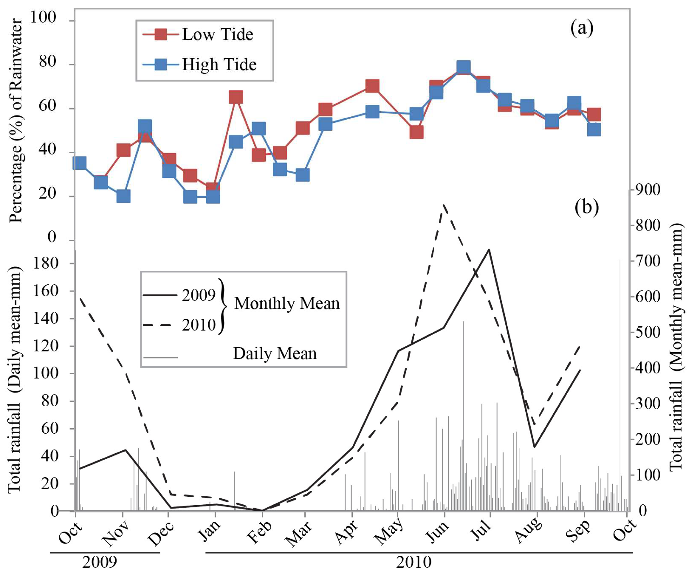
The region receives rainfall distributed across three distinct rainfall seasons and is characterized by unique isotopic ratios [37,38,40]. The monthly mean and daily rainfall data of the study location (Willingdon weather station, located within ~3 km of the site of monthly tidal surface water collection) indicated that in almost all years, rainfall is maximum from June to August, coinciding with the SW Monsoon (Figure 5—bottom panel). Based on the amount of rainfall and δ¹⁸O offset, the percentage contribution of freshwater was estimated for HT and LT sampling and is shown in Figure 5 (top panel). It was evident that freshwater flux into the CBW estuary is primarily driven by runoff, which is a major contributor during the SWM season but drops significantly during the Premonsoon and Postmonsoon periods. The water δ¹⁸O values of seasonal surface water were adapted from the tropical Chaliyar River basin to constrain the end member composition. The catchment area of this river is the Western Ghats region in India, which receives rainfall from the source that feeds the rivers flowing into the CBW [34]. The surface water δ¹⁸O values for the Chaliyar river were −1.8‰, −1.2‰, and −4.5‰ for the NEM, Premonsoon, and SWM seasons. respectively [39], and the corresponding freshwater percentages estimated using Equation (6) were 20–52% during the NEM season, 53–67% during the Premonsoon season, and 42–80% during the SWM season, similar to earlier reported studies [41].

3.4. Performance Metrics for ML Models

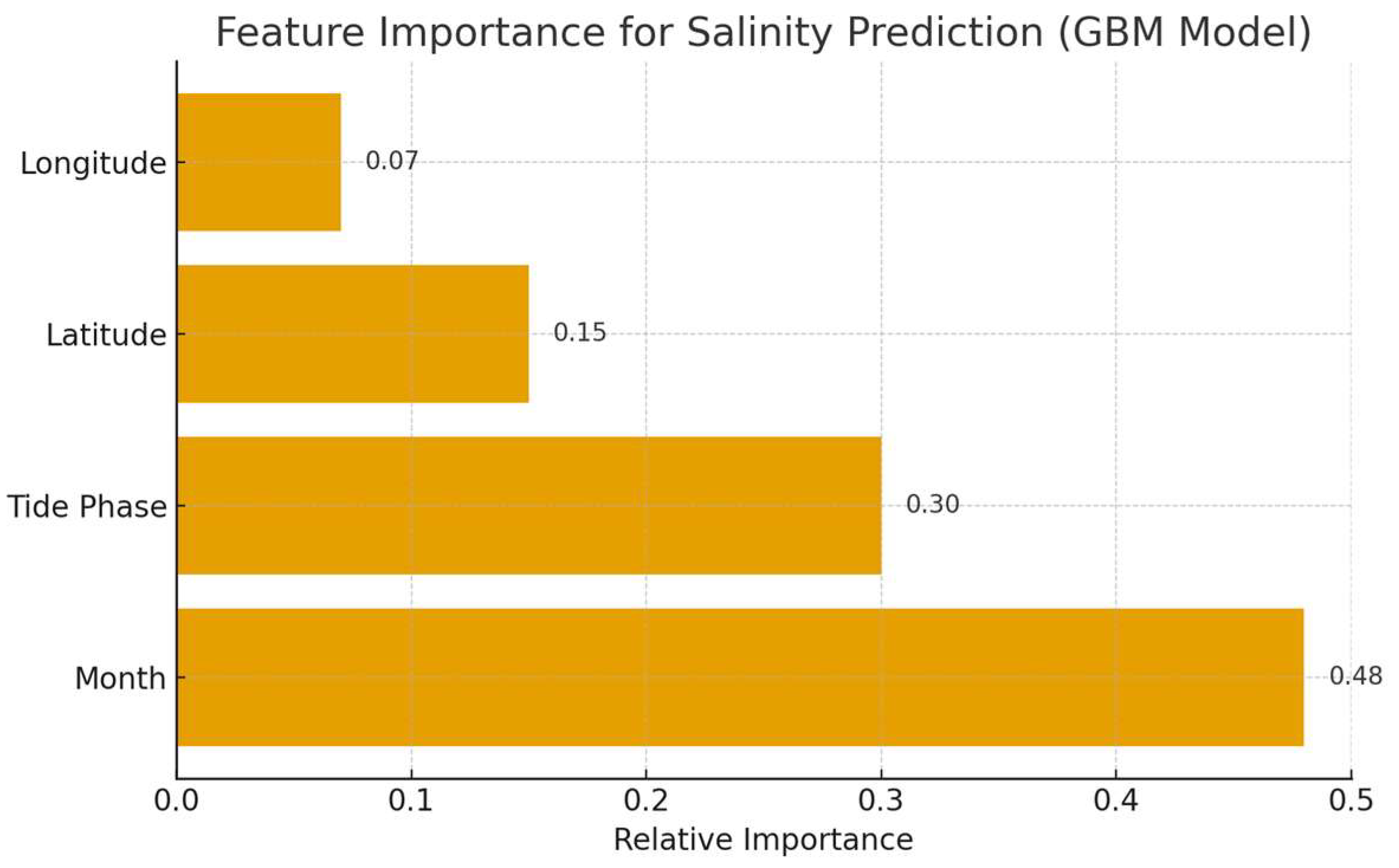
The performance metrics of all the used ML models are summarized in

Table 4. Performance metrics of all ML models used in this study and the target parameters modeled.

Model	Target	RMSE	R2	MAPE (%)	T-Test (p-Value)
GBM	Salinity	0.0993	0.9563	N/A	<0.001
GPR	δ18O	0.6298	−5.7860	N/A	0.045
CART	δ13C	0.3449	−2.0460	N/A	0.089
ELM	δ18O	0.9187	−13.440	N/A	0.103
ELM	δ13C	0.7626	−13.890	N/A	0.097
RBNN	δ18O	0.2869	−0.4080	N/A	<0.001
RBNN	δ13C	0.2626	−0.7660	N/A	<0.001
RF	δ18O	0.2101	0.2451	36.19	<0.001
RF	δ13C	0.2489	−0.5869	34.90	0.032
SVM	δ18O	0.2500	−0.0695	39.16	0.071
SVM	δ13C	0.2556	−0.6722	25.88	0.089
KNN	δ18O	0.1703	0.5039	29.87	<0.001

. The results revealed a stark difference in model predictability across the three target parameters (salinity, δ¹⁸O, and δ¹³C). For salinity prediction, the GBM model showed the highest accuracy, with the lowest RMSE (0.0993) and the highest R² (0.9563, p-value: <0.001). For δ¹⁸O prediction, the KNN model performed best, achieving an RMSE of 0.1703, an R² of 0.5039, and a MAPE of 29.87%. The RF model also showed acceptable performance (RMSE: 0.2101, R²: 0.2451, p-value: <0.001), while several other models, including SVM, GPR, and RBNN, failed entirely, producing negative R² values. For δ¹³C prediction, models such as CART, ELM, and RBNN performed poorly, with negative R² values suggesting overfitting or insufficient training data. A key advantage of tree-based models like GBM is their ability to provide insights into the drivers of their predictions through feature importance rankings. For our best performing model (GBM for salinity prediction), we analyzed these scores to identify the most influential hydrographic parameters. As illustrated in the bar chart in Figure 6, temporal factors were the dominant predictors. The month of the year, which serves as a proxy for the monsoon cycle, was the single most important feature, followed by the tidal phase. This finding aligns with our understanding of the estuary, where seasonal freshwater influx and tidal exchange are the primary drivers of salinity variation. Geographic location (latitude and longitude) also contributed to the prediction but was of secondary importance.

It is important to note that in models like GPR, CART, and RBNN negative R² values were obtained, and this poor performance may be attributed to their sensitivity to small datasets and high feature noise, which often leads to overfitting or underfitting, as observed in our limited dataset. Additionally, certain input features may have limited predictive powers affecting the models more severely. A clearer analysis of feature importance and model complexity would provide valuable insights into these performance discrepancies. Furthermore, there exists a necessity for further dataset expansion and model refinement using additional ecological and geochemical variables.

4. Discussion

4.1. Seasonal and Spatial Variations in δ¹⁸O and Salinity

The salinity–δ¹⁸O relationship is a valuable tool for understanding the temporal mixing pattern of freshwater and seawater in estuaries around the world [42,43,44]. The surface-water salinity–oxygen isotopes of CBW showed two distinct trends defining the summer and winter composition. This large difference between salinity and water δ¹⁸O is due to the mixing of a variable amount of fresh water by the rivers draining the catchment and the saline Arabian Sea water. The rainwater δ¹⁸O during the monsoon season dominates the river water value, which varies between −1.0‰ and −3‰, while groundwater remains nearly invariant seasonally with a composition maximally ranging from −3.7 to −5.2‰ in the region [39]. The δ¹⁸O value of the seawater input into the estuary is isotopically heavier, with values between 1 and 0‰ in the Arabian Sea region. The difference between the salinity values measured during high and low tides was maximum during the summer season and minimum during the monsoon season. This implies that the extent of mixing of surface water is maximum in the monsoon season and minimum in the summer. The overall average empirical relationship between water δ¹⁸O and salinity for the CBW was δ¹⁸O = 0.1259 (Salinity) −3.31, with a strong regression coefficient value of 0.7 (Figure 7). One-sided ANOVA was carried out to understand the significance of the δ¹⁸O–salinity relationship, and the obtained statistical summary, indicating robustness of the regression lines, is given in Supplementary Table S1. Our observed δ¹⁸O–salinity relationship was similar to other monsoon estuaries in the Indian monsoon region, with a slightly lower slope for the Mandovi-Zuari [18] and Hooghly estuaries [13].

4.2. δ¹⁸O and δ¹³C Relationship with Salinity

Surface water salinity depends mainly on freshwater drainage, which carries a signature of rainwater during the wet period and groundwater during the dry period. The annual observed salinity varies from 21.7 to 0.1 (Table 1), with the lowest surface salinity coinciding with a period of the SWM, where precipitation and catchment runoff reach their maximum. Maximum observed salinity was in the Premonsoon period, wherein seawater intrusion was prominent. It was evident that the CBW region experienced diurnal and monthly tidal influences, which varied seasonally with the extent of seawater intrusion into the coastal area.

The tidal influence and sea water intrusion strongly stratify the CBW estuary, leading to the observed spatial zonation (Zone 1 to 3; Figure 4 left panel) observed in the measured hydrochemical parameters (Table 2) and presented in Section 3.2. In Zone 1, the region from the Cochin Inlet to Perumpalam Island, the influence of seawater from the Arabian Sea is pronounced with a δ¹⁸O–salinity relationship slope of 0.03 and a positive correlation (R² = 0.37). Zone 2, from Perumpalam Island to Thanneermukkam Bund, exhibits the mixing of freshwater from riverine input and seawater from the Arabian Sea with a steep slope of 0.5 and a strong positive correlation (R² = 0.6). Zone 3 is dominated by freshwater influx and evaporative effects, as seen in Figure 4 (left panel), and had a negative slope of −0.9 with insignificant correlation (R² = 0.05). A summary table of various parameters in each of these zones is given in Supplementary Table S2. It is important to note that this classification of zones is spatial and not temporal. In addition, further studies with expanded sampling and statistical validation are needed to accurately delineate freshwater input zones and establish robustness.

4.3. δ¹⁸O–δD Relationship of CBW Estuary

A total of 17 surface water samples collected during the Premonsoon season were analyzed for δD and δ¹⁸O to understand the δ¹⁸O–δD relationship. The results are plotted in Figure 8 along with measurements from previously published studies in the region [14], in addition to both the Global Meteoric Water Line (GMWL) and Local Meteoric Water Line (LMWL) from the published literature [40]. In the previous study documenting the stable isotopic values of Vembanad Lake water samples, the reported values were −20.2 to +17.0‰ and −5.6 to +3.3‰ for δD and δ¹⁸O, respectively [14]. The most isotopically depleted values were observed during the monsoon season, which could be attributed to the amount effect. In contrast, an enrichment in isotopic values was observed during the Premonsoon period due to salinity mixing or evaporation. In our study, we carried out spatial sampling only during the Premonsoon season, and the δD vs. δ¹⁸O plot was characterized by enriched δ values similar to earlier observations, as shown in Figure 8 [14]. The ingression of saline seawater with enriched isotope values also contributed to overall isotope observations in the CBW estuary. The gradual decrease in δ¹⁸O and δD values observed within even a single Premonsoon season indicates either excess evaporation or an enhanced contribution of seawater, causing a compositional shift during the Premonsoon season.

4.4. Carbon Dynamics Using Salinity and δ¹³C_DIC

Freshwater input to the estuary affects the net carbon isotopic composition of dissolved inorganic carbon, which is either derived from the degradation of organic matter present in the regional soil ecosystem or further modified due to water column productivity. Thus, δ¹³C_DIC can act as a proxy for productivity in estuarine systems. However, the inorganic carbon reservoir in estuary water can vary across seasons, recording the flux of carbon due to silicate weathering [45]. The δ¹³C_DIC observed during the present study ranged from −2.9‰ to −21.3‰, with an average δ¹³C_DIC of −10.4‰. These obtained values are comparable with a previous study of δ¹³C_DIC in the region [19]. Figure 4 (right panel) shows the conservative mixing curve of δ¹³C_DIC, along with the respective actual values and salinity in the three different spatial zones that were identified and defined in this study for the CBW estuary (Figure 4, right panel). Among the five stations sampled in Zone 1, four stations were closest to the estimated conservative mixing line, indicating the role of the mixing of freshwater and seawater end members. The samples from Zone 2 were characterized by lower δ¹³C_DIC values relative to the respective conservative mixing curve values (Figure 4, right panel). As observed in previous studies [19,45], the possible reason for the low δ¹³C_DIC at these stations might be the dominant contribution from terrestrial inorganic carbon from the degradation of organics. The samples from Zone 3 were characterized by the lowest δ¹³C_DIC relative to the respective conservative mixing curves. This indicates that the carbon dynamics in Zone 3 are dictated by processes like runoff from the nearby paddy fields with a lighter C₃ signature (−25‰), which is further modified owing to the productivity of the estuary [19,46], resulting in δ¹³C_DIC values ranging from −13 to −21‰. This is further evidenced by higher nutrients (nitrate, phosphate, silicate) in this zone during the monsoon and Postmonsoon season [47].

4.5. Evaluating ML Models for Salinity and Stable Isotopic Prediction

This study compared multiple machines learning models, including GBM, KNN, RF, SVM, CART, ELM, and RBNN, to predict salinity and isotopic ratios. The comparison of various machine learning models highlights the challenges and opportunities in predicting salinity and isotopic compositions [20,21]. The varying success of the machine learning models in predicting salinity, δ¹⁸O, and δ¹³C offers significant insights into not only the models themselves but also the fundamental nature of the processes governing each parameter. The GBM model emerged as the most reliable for salinity prediction, demonstrating the highest accuracy and predictive strength (Table 4). Salinity in the estuary, while dynamic, behaves conservatively and is a direct function of the mixing ratio between freshwater and seawater. This ratio is strongly governed by predictable spatial (latitude, longitude) and temporal (month, tidal phase) factors. The GBM model, with its tree-based architecture, excels at capturing this complex, non-linear, but deterministic relationship, making it an ideal tool for this parameter.

For δ¹⁸O prediction, the KNN model outperformed others, although overall performance metrics indicated room for improvement. δ¹⁸O variability is largely controlled by conservative mixing, but it is subject to additional, localized processes like evaporation. The KNN algorithm, which makes predictions based on the values of its ‘neighbors’, is well-suited to capturing such strong spatial autocorrelation. However, the fact that even the best model could only explain 50% of the variance highlights a key limitation: our input features do not account for stochastic factors like the variable isotopic composition of individual rainfall events, which introduces noise that the model cannot possibly resolve. The low performance of models like SVM for δ¹⁸O prediction suggests that certain ML approaches may not be well-suited for isotopic modeling without extensive parameter tuning and preprocessing (Table 4). The success of GBM/KNN models in salinity and δ¹⁸O prediction with acceptable correlation values and significant p-values (p-value: <0.001) could be attributed to the capturing of tidal hysteresis effects via lagged salinity features and evaporation enrichment through latitude–temperature interactions (feature importance > 0.85). This aligns with studies where tree-based models outperformed SVMs in monsoon-driven estuaries [21,27].

δ¹³C prediction faced significant challenges, with all tested models failing to produce a meaningful predictive relationship, as indicated by the negative R² values (Table 4). A negative R² indicates that the model’s predictions are worse than a simple baseline model that always predicts the mean of the target variable, signifying a complete failure of the model to generalize. This outcome is a critical finding of our study and is not merely an issue of dataset size, but rather a result of cascading issues stemming from both the data and the modeling process itself. The primary cause is the absence of key biogeochemical predictor variables in our dataset, leading to a very low signal-to-noise ratio. From a machine learning perspective, this leads to several technical failures:

• Severe Overfitting: Flexible models, in an attempt to find a pattern, likely learned the random noise within the training data. This results in a model that is perfectly tuned to the training set but has no predictive power on unseen data.
• Unsuitable Model Architecture: The complex and potentially discontinuous nature of δ¹³C dynamics may require more specialized model architectures than those tested. The ‘step-function’ discontinuities introduced by biological fractionation are particularly challenging for standard regression algorithms.
• Hyperparameter Tuning Failure: In a low-signal environment, the Bayesian optimization process is susceptible to finding a ‘fluke’ set of hyperparameters that perform well on the validation set by chance but fail to capture any generalizable relationship, leading to the observed poor performance on the final test set.

Strong correlation between δ¹⁸O and salinity reinforces the utility of isotopes in tracing hydrochemical processes. Geographic parameters could also play a crucial role in model performance, indicating spatial influences on isotopic variations. The findings emphasize that while ML can be a powerful tool for hydrochemical predictions, robust data collection and model refinement are essential to improve generalizability and reliability across different environmental conditions. In addition, robust data collection, by means of future extended sampling campaigns spatially and temporally, and understanding tidal influences are essential to further constrain and understand the biogeochemical zone stratification discussed here.

5. Conclusions

This study provides the first combined application of stable isotopes and machine learning (ML) models to quantify seasonal freshwater inflows into the Cochin Backwater (CBW) estuary. The summary of the key findings of the study are as follows: (1) Seasonal Hydrography: The δ¹⁸O–salinity relationship (δ¹⁸O = 0.1259 × Salinity − 3.31; R² = 0.7) clearly captured the seasonal freshwater–seawater mixing dynamics. Freshwater contributions were highest during the Southwest Monsoon (42–80%), moderate during the Pre-monsoon (53–67%), and lowest during the Northeast Monsoon (20–52%). (2) Spatial Estuarine Zonation: Spatial surveys during the Premonsoon identified three distinct hydro-biogeochemical zones: Zone 1: Dominated by seawater with heavier δ¹³C signatures; Zone 2: Mixed inputs from rivers and terrestrial sources; and Zone 3: Strong influence of paddy field runoff and estuarine productivity, marked by lighter δ¹³C values. (3) Carbon Dynamics: δ¹³C_DIC analysis revealed clear spatial heterogeneity, reflecting the combined influence of seawater mixing, terrestrial carbon input, and agricultural runoff. (4) Among the eight ML models tested, Gradient Boosting Machine (GBM) showed the highest accuracy for salinity prediction (R² = 0.96), while K-Nearest Neighbor (KNN) performed best for δ¹⁸O (R² = 0.50). In contrast, δ¹³C predictions with ML models were unsuccessful due to the absence of key biogeochemical drivers in the dataset. Overall, this study demonstrates that coupling stable isotope geochemistry with ML models provides a powerful framework for quantifying seasonal freshwater fluxes and estuarine zonation in monsoon-regulated systems. The approach offers a scalable pathway for predictive modeling under changing climatic and anthropogenic pressures and can inform better management and conservation of tropical estuarine ecosystems.

References

1. Day, J.W., Jr.; Kemp, W.M.; Yáñez-Arancibia, A.; Crump, B.C. (Eds.) Estuarine Ecology; John Wiley & Sons: Hoboken, NJ, USA, 2012. [Google Scholar]
2. Dittmar, T.; Lara, R.J. Driving forces behind nutrient and organic matter dynamics in a mangrove tidal creek in North Brazil. Estuar. Coast. Shelf Sci. 2001, 52, 249–259. [Google Scholar] [CrossRef]
3. Cloern, J.E.; Jassby, A.D. Patterns and scales of phytoplankton variability in estuarine–coastal ecosystems. Estuaries Coasts 2010, 33, 230–241. [Google Scholar]
4. Vijith, V.; Sundar, D.; Shetye, S.R. Time-dependence of salinity in monsoonal estuaries. Estuar. Coast. Shelf Sci. 2009, 85, 601–608. [Google Scholar] [CrossRef]
5. Qasim, S.; Gopinathan, C. Tidal cycle and the environmental features of Cochin Backwater (a tropical estuary). Proc. Indian Acad. Sci. Sect. A Part 3 Math. Sci. 1969, 69, 336–348. [Google Scholar]
6. Haldar, R.; Khosa, R.; Gosain, A.K. Impact of Anthropogenic Interventions on the Vembanad Lake System. In Water Resources and Environmental Engineering I; Rathinasamy, M., Chandramouli, S., Phanindra, K., Mahesh, U., Eds.; Springer: Singapore, 2019. [Google Scholar]
7. Kulk, G.; George, G.; Abdulaziz, A.; Menon, N.; Theenathayalan, V.; Jayaram, C.; Brewin, R.J.; Sathyendranath, S. Effect of Reduced Anthropogenic Activities on Water Quality in Lake Vembanad, India. Remote Sens. 2020, 13, 1631. [Google Scholar] [CrossRef]
8. Pranav, P.; Roy, R.; Jayaram, C.; D’Costa, P.M.; Choudhury, S.B.; Menon, N.N.; Nagamani, P.; Sathyendranath, S.; Abdulaziz, A.; Sai, M.S.; et al. Seasonality in carbon chemistry of Cochin backwaters. Reg. Stud. Mar. Sci. 2021, 46, 101893. [Google Scholar] [CrossRef]
9. Shivaprasad, A.; Vinita, J.; Revichandran, C.; Reny, P.D.; Deepak, M.P.; Muraleedharan, K.R.; Naveen Kumar, K.R. Seasonal stratification and property distributions in a tropical estuary (Cochin estuary, west coast, India). Hydrol. Earth Syst. Sci. 2013, 17, 187–199. [Google Scholar] [CrossRef]
10. Balachandran, K.K.; Joseph, T.; Nair, K.K.C.; Nair, M.; Joseph, P.S. The Complex Estuarine Formation of Six Rivers (Cochin Backwaters System on West Coast of India)—Sources and Distribution of Trace Metals and Nutrients. 2002. Available online: https://drs.nio.org/drs/handle/2264/1340 (accessed on 30 August 2025).
11. Sankaranarayanan, V.N.; Qasim, S.Z. Nutrients of the Cochin Backwater in relation to environmental characteristics. Mar. Biol. 1969, 2, 236–247. [Google Scholar] [CrossRef]
12. Aneesh, T.D.; Srinivas, R.; Singh, A.T.; Resmi, T.R.; Nair, A.M.; Redkar, B.L. Stable water isotope signatures of dual monsoon precipitation: A case study of Greater Cochin region, south-west coast of India. J. Earth Syst. Sci. 2019, 128, 210. [Google Scholar] [CrossRef]
13. Ghosh, P.; Chakrabarti, R.; Bhattacharya, S.K. Short- and long-term temporal variations in salinity and the oxygen, carbon and hydrogen isotopic compositions of the Hooghly Estuary water, India. Chem. Geol. 2013, 335, 118–127. [Google Scholar] [CrossRef]
14. Nasir, U.P.; Harikumar, P.S. Hydrochemical and isotopic investigation of a tropical wetland system in the Indian sub-continent. Environ. Earth Sci. 2012, 66, 111–119. [Google Scholar]
15. Bhavya, P.S.; Kumar, S.; Gupta, G.V.M.; Sudharma, K.V.; Sudheesh, V.; Dhanya, K.R. Carbon isotopic composition of suspended particulate matter and dissolved inorganic carbon in the Cochin estuary during post-monsoon. Curr. Sci. 2016, 110, 1539–1543. [Google Scholar]
16. Raymond, P.A.; Bauer, J.E.; Caraco, N.F.; Cole, J.J.; Longworth, B.; Petsch, S.T. Controls on the variability of organic matter and dissolved inorganic carbon ages in northeast US rivers. Mar. Chem. 2004, 92, 353–366. [Google Scholar] [CrossRef]
17. Bouillon, S.; Borges, A.V.; Castañeda-Moya, E.; Diele, K.; Dittmar, T.; Duke, N.C.; Kristensen, E.; Lee, S.Y.; Marchand, C.; Middelburg, J.J.; et al. Mangrove production and carbon sinks: A revision of global budget estimates. Glob. Biogeochem. Cycles 2008, 22, GB2013. [Google Scholar] [CrossRef]
18. Ghosh, P.; Ramdas, L.; Banerjee, Y.; Thamizharasan, S.; Banerjee, S. Seasonal freshwater flux estimation using mollusc from the tropical Mandovi Zuari estuary, Goa, India. J. Earth Syst. Sci. 2021, 130, 107. [Google Scholar] [CrossRef]
19. Bhavya, P.S.; Kumar, S.; Gupta, G.V.M.; Sudharma, K.V.; Sudheesh, V. Spatio-temporal variation in δ13C-DIC of a tropical eutrophic estuary (Cochin estuary, India) and adjacent Arabian Sea. Cont. Shelf Res. 2018, 153, 75–85. [Google Scholar] [CrossRef]
20. Astray, G.; Soto, B.; Barreiro, E.; Gálvez, J.F.; Mejuto, J.C. Machine learning applied to the oxygen-18 isotopic composition, salinity and temperature/potential temperature in the Mediterranean Sea. Mathematics 2021, 9, 2523. [Google Scholar] [CrossRef]
21. Cemek, B.; Arslan, H.; Küçüktopcu, E.; Simsek, H. Comparative analysis of machine learning techniques for estimating groundwater deuterium and oxygen-18 isotopes. Stoch. Environ. Res. Risk Assess. 2022, 36, 4271–4285. [Google Scholar] [CrossRef]
22. Noori, N.; Kalin, L.; Isik, S. Water quality prediction using SWAT-ANN coupled approach. J. Hydrol. 2020, 590, 125220. [Google Scholar] [CrossRef]
23. Ly, Q.V.; Nguyen, X.C.; Lê, N.C.; Truong, T.D.; Hoang, T.H.T.; Park, T.J.; Maqbool, T.; Pyo, J.-C.; Cho, K.H.; Lee, K.-S.; et al. Application of machine learning for eutrophication analysis and algal bloom prediction in an urban river: A 10-year study of the Han River, South Korea. Sci. Total Environ. 2021, 797, 149040. [Google Scholar]
24. Samalavičius, V.; Gadeikienė, S.; Žaržojus, G.; Gadeikis, S.; Lekstutytė, I. Oxygen-18 prediction using machine learning in the Baltic Artesian Basin groundwater. Stoch. Environ. Res. Risk Assess. 2024, 39, 765–787. [Google Scholar] [CrossRef]
25. Albuquerque, L.G.; de Oliveira Roque, F.; Valente-Neto, F.; Koroiva, R.; Buss, D.F.; Baptista, D.F.; Hepp, L.U.; Kuhlmann, M.L.; Sundar, S.; Covich, A.P.; et al. Large-scale prediction of tropical stream water quality using Rough Sets Theory. Ecol. Inform. 2021, 61, 101226. [Google Scholar] [CrossRef]
26. Al Sudani, Z.A.; Salem, G.S.A. Evaporation rate prediction using advanced machine learning models: A comparative study. Adv. Meteorol. 2022, 2022, 1433835. [Google Scholar] [CrossRef]
27. Dagher, D.H. Assessment of using machine and deep learning applications in surface water quantity and quality predictions: A review. J. Water Resour. Geosci. 2024, 3, 18–48. [Google Scholar]
28. Van Binh, D. Reconstructing Daily Discharge in a Megadelta Using Machine Learning Techniques. Water Resour. Res. 2022, 58, e2021WR031048. [Google Scholar] [CrossRef]
29. Downing, B.D.; Bergamaschi, B.A.; Kendall, C.; Kraus, T.E.C.; Dennis, K.J.; Carter, J.A.; von Dessonneck, T.S. Using Continuous Underway Isotope Measurements to Map Water Residence Time in Hydrodynamically Complex Tidal Environments. Environ. Sci. Technol. 2016, 50, 13387–13396. [Google Scholar] [CrossRef] [PubMed]
30. Singh, A.; Jani, R.A.; Ramesh, R. Spatiotemporal variations of the δ18O-salinity relation in the northern Indian Ocean. Deep Sea Res. Part I Oceanogr. Res. Pap. 2010, 57, 1422–1431. [Google Scholar] [CrossRef]
31. Deshpande, R.D.; Muraleedharan, P.M.; Singh, R.L.; Kumar, B.; Rao, M.S.; Dave, M.; Sivakumar, K.U.; Gupta, S.K. Spatio-temporal distributions of δ18O, δD and salinity in the Arabian Sea: Identifying processes and controls. Mar. Chem. 2013, 157, 144–161. [Google Scholar] [CrossRef]
32. Rasheed, K.; Joseph, K.A.; Balchand, A.N. Impacts of harbour dredging on the coastal shoreline features around Cochin. In Proceedings of the International Conference on Coastal Change, Bordeaux, France, 10–16 February 1995; pp. 943–948. [Google Scholar]
33. Epstein, S.; Mayeda, T. Variation of O18 content of waters from natural sources. Geochim. Cosmochim. Acta 1953, 4, 213–227. [Google Scholar] [CrossRef]
34. Rangarajan, R.; Ghosh, P. Role of water contamination within the GC column of a GasBench II peripheral on the reproducibility of 18O/16O ratios in water samples. Isot. Environ. Health Stud. 2011, 47, 498–511. [Google Scholar] [CrossRef]
35. Assayag, N.; Rivé, K.; Ader, M.; Jézéquel, D.; Agrinier, P. Improved method for isotopic and quantitative analysis of dissolved inorganic carbon in natural water samples. Rapid Commun. Mass Spectrom. 2006, 20, 2243–2251. [Google Scholar] [CrossRef]
36. Rangarajan, R.; Pathak, P.; Banerjee, S.; Ghosh, P. Floating boat method for carbonate stable isotopic ratio determination in a GasBench II peripheral. Rapid Commun. Mass Spectrom. 2021, 35, e9115. [Google Scholar]
37. Lekshmy, P.R.; Midhun, M.; Ramesh, R.; Jani, R.A. 18O depletion in monsoon rain relates to large-scale organized convection rather than the amount of rainfall. Sci. Rep. 2014, 4, 5661. [Google Scholar] [CrossRef]
38. Rahul, P.; Ghosh, P. Long term observations on stable isotope ratios in rainwater samples from twin stations over Southern India; identifying the role of amount effect, moisture source and rainout during the dual monsoons. Clim. Dyn. 2019, 52, 6893–6907. [Google Scholar] [CrossRef]
39. Hameed, A.S.; Resmi, T.R.; Suraj, S.; Warrier, C.U.; Sudheesh, M.; Deshpande, R.D. Isotopic characterization and mass balance reveals groundwater recharge pattern in Chaliyar river basin, Kerala, India. J. Hydrol. Reg. Stud. 2015, 4, 48–58. [Google Scholar] [CrossRef]
40. Warrier, C.U.; Babu, M.P.; Manjula, P.; Velayudhan, K.T.; Hameed, A.S.; Vasu, K. Isotopic characterization of dual monsoon precipitation—Evidence from Kerala, India. Curr. Sci. 2010, 99, 1487–1495. [Google Scholar]
41. Seena, G.; Muraleedharan, K.R.; Revichandran, C.; Abdul Azeez, S.; John, S. Seasonal spreading and transport of buoyant plumes in the shelf off Kochi, southwest coast of India—A modeling approach. Sci. Rep. 2019, 9, 19956. [Google Scholar] [CrossRef] [PubMed]
42. Torgersen, T. Isotopic composition of river runoff on the US East Coast: Evaluation of stable isotope versus salinity plots for coastal water mass identification. J. Geophys. Res. Ocean 1979, 84, 3773–3775. [Google Scholar] [CrossRef]
43. Fairbanks, R.G.; Sverdlove, M.; Free, R.; Wiebe, P.H.; Bé, A.W. Vertical distribution and isotopic fractionation of living planktonic foraminifera from the Panama B—Asin. Nature 1982, 298, 841. [Google Scholar] [CrossRef]
44. Khim, B.-K.; Park, B.-K.; Yoon, H.-I. Oxygen isotopic compositions of seawater in the Maxwell Bay of King George Island, west Antarctica. Geosci. J. 1997, 1, 115. [Google Scholar] [CrossRef]
45. Samanta, S.; Dalai, T.K.; Tiwari, S.K.; Rai, S.K. Quantification of source contributions to the water budgets of the Ganga (Hooghly) River estuary, India. Mar. Chem. 2018, 207, 42–54. [Google Scholar] [CrossRef]
46. Kaushal, R.; Ghosh, P.; Geilmann, H. Fingerprinting environmental conditions and related stress using stable isotopic composition of rice (Oryza sativa L.) grain organic matter. Ecol. Indic. 2016, 61, 941–951. [Google Scholar] [CrossRef]
47. Nagarathinam, A.; Retnamma, J.; Loganathan, J.; Singaram, P.; Madam, S.M.K.; Jose, A.K.; Subramanian, P.R. Implications of an extensive salt water barrage on the distribution of black clam in a tropical estuarine system, Southwest coast of India. Oceanologia 2021, 63, 343–355. [Google Scholar] [CrossRef]
Figure 1. Map of Cochin Backwater with sampling locations. The temporal sampling location is denoted by a filled circle (samples in Table 1), whereas hollow circles represent the locations of spatial sampling (samples in Table 2).
Hydrology 12 00277 g001
Figure 2. Workflow of advanced ML techniques that were employed to estimate and predict δ18O and δ13C isotopic compositions and salinity in the estuary.
Hydrology 12 00277 g002
Figure 3. The top panel shows high and low tide water δ18O, while the bottom panel shows salinity data of the collected water samples. Filled and hollow squares represent δ18O values of high and low tide, respectively. Filled and hollow diamonds represent salinity values of high and low tide, respectively (Green Region—NEM; Light Pink—PM; Gray—SWM).
Hydrology 12 00277 g003
Figure 4. (a) δ18O–salinity relationship indicating three different spatial zones for collected Premonsoon samples depicted by hollow red squares, green triangles, and purple diamonds representing δ18O and salinity values from Zones 1, 2, and 3, respectively. (b) δ13C–salinity relationship of the spatial zones along with the conservative mixing curve. Hollow red squares, green triangles, and purple diamonds represent δ13C and salinity values from Zones 1, 2, and 3, respectively, while hollow black circles and the corresponding dotted line represent the conservative mixing curve. The grey circles in both (a,b) refers to the identified zonation’s in the estuary.
Hydrology 12 00277 g004
Figure 5. (a) Relative contribution of freshwater to the Cochin Backwater at different times of the year calculated using the δ18O of the freshwater end member and seawater. Red and blue squares represent the percentage of rainwater at low and high tide, respectively. (b) Monthly (continuous and broken black line) and daily (gray) mean rainfall in mm.
Hydrology 12 00277 g005
Figure 6. Feature importance for salinity prediction. The relative importance of predictor variables as determined by the Gradient Boosting Machine (GBM) model. Importance is calculated as the mean decrease in impurity; higher values indicate greater importance.
Hydrology 12 00277 g006
Figure 7. Correlation plot between δ18O and salinity in the collected CBW samples indicating the mixing between freshwater and saline water (VSMOW—Vienna Standard Mean Ocean Water). Hollow green and red squares represent δ18O and salinity values of high and low tide, respectively, whereas filled gray circles represent the average value.
Hydrology 12 00277 g007
Figure 8. Comparison of the δ18O–δD regression line based on 18 Premonsoon surface water samples (Table 1) collected and compared with the Global Meteoric Water Line (GMWL) and Local Meteoric Water Line (LMWL) from published literature (Nasir and Harikumar, 2012 [14] and Warrier et al., 2010 [41]).
Hydrology 12 00277 g008