Article

Enhanced 3D Turbulence Models Sensitivity Assessment Under Real Extreme Conditions: Case Study, Santa Catarina River, Mexico

by
Mauricio De la Cruz-Ávila
and
Rosanna Bonasia
*
School of Engineering and Sciences, Tecnologico de Monterrey, Carretera Lago de Guadalupe Km 3.5 Atizapán de Zaragoza Col. Margarita Maza de Juárez, Cd López Mateos 52926, Mexico
*
Author to whom correspondence should be addressed.
Hydrology 2025, 12(10), 260; https://doi.org/10.3390/hydrology12100260
Submission received: 1 September 2025 / Revised: 26 September 2025 / Accepted: 28 September 2025 / Published: 2 October 2025

Abstract

This study compares enhanced turbulence models in a natural river channel 3D simulation under extreme hydrometeorological conditions. Using ANSYS Fluent 2024 R1 and the Volume of Fluid scheme, five RANS closures were evaluated: realizable k–ε, Renormalization-Group k–ε, Shear Stress Transport k–ω, Generalized k–ω, and Baseline-Explicit Algebraic Reynolds Stress model. A segment of the Santa Catarina River in Monterrey, Mexico, defined the computational domain, which produced high-energy, non-repeatable real-world flow conditions where hydrometric data were not yet available. Empirical validation was conducted using surface velocity estimations obtained through high-resolution video analysis. Systematic bias was minimized through mesh-independent validation (<1% error) and a benchmarked reference closure, ensuring a fair basis for inter-model comparison. All models were realized on a validated polyhedral mesh with consistent boundary conditions, evaluating performance in terms of mean velocity, turbulent viscosity, strain rate, and vorticity. Mean velocity predictions matched the empirical value of 4.43 [m/s]. The Baseline model offered the highest overall fidelity in turbulent viscosity structure (up to 43 [kg/m·s]) and anisotropy representation. Simulation runtimes ranged from 10 to 16 h, reflecting a computational cost that increases with model complexity but justified by improved flow anisotropy representation. Results show that all models yielded similar mean flow predictions within a narrow error margin. However, they differed notably in resolving low-velocity zones, turbulence intensity, and anisotropy within a purely hydrodynamic framework that does not include sediment transport.

1. Introduction

Numerical simulations of fluvial environments have become essential tools for hydrodynamic analysis [1,2], flood prediction [3,4,5], river engineering [4], and ecological management [6,7]. Computational Fluid Dynamics (CFD) approaches enable the detailed characterization of complex flow structures, particularly under unsteady and three-dimensional conditions that are difficult to capture using traditional analytical or empirical models [8,9,10]. Although 2D shallow-water models remain common in tools such as IBER [11] or HEC-RAS [12], they rely on assumptions of hydrostatic pressure and depth-averaged velocities. These assumptions limit their accuracy in resolving vertical flow structures, secondary currents, and turbulence-dominated regions near obstructions or irregular bed morphologies [13,14,15,16,17].
Riverine simulations differ from internal flow applications in several fundamental aspects. First, the domain typically exhibits large aspect ratios and complex bathymetry [3,18], necessitating unstructured meshes that conform to sub-meter bedforms while spanning kilometer-scale reaches [19,20,21]. Second, the presence of a deformable water–air interface introduces additional non-linearity, requiring robust Volume of Fluid (VoF) [22] or Level-Set algorithms [23]. Third, field validation data are limited to surface velocities [24,25], stage–discharge curves [26,27,28,29], or sparse Acoustic Doppler current profilers (ADCP) transects [30,31,32], making it difficult to verify turbulence metrics. In addition to these aspects, other challenges must be considered, such as sediment–flow interactions that alter streambed geometries, non-Newtonian effects arising in highly turbid flows, and time-varying boundary conditions associated with flood waves. Consequently, selecting an appropriate turbulence model becomes not only a matter of balancing computational cost against the level of physical detail required by the application (e.g., bulk discharge prediction versus bed shear stress estimation) but also of ensuring that energy dissipation is realistically captured in regions where the physical complexity is highest. Misrepresentation of turbulence behavior under these conditions can lead to substantial errors in simulated velocity fields, shear stress distributions, and sediment transport predictions, particularly when validation data are sparse or indirect.
3D CFD has become an indispensable tool for predicting flow behavior in natural waterways [20,33], informing flood risk management, river-engineering design, and habitat assessment [34]. Over the past decade, considerable progress has been made in coupling unsteady Reynolds-averaged Navier–Stokes (URANS) solvers with high-resolution topographic datasets, enabling researchers to simulate meter-scale turbulence in domains with Reynolds numbers exceeding 109 [35,36]. However, despite these advances, turbulence closure remains a dominant source of model uncertainty [37,38,39,40,41,42]. Traditional RANS-based models, such as the standard k     ε and k     ω formulations, are computationally efficient but rely on isotropy assumptions and fixed constants, which limit their accuracy in predicting secondary currents, boundary-layer separation, and free-surface deformation in complex river geometries [15,43,44,45,46].
Although widely used as default options in commercial solvers, conventional models fail to capture flow anisotropy, streamline curvature, and near-wall dynamics in natural rivers [13,47,48]. To address these deficiencies, enhanced closures have been proposed, including the k ε Renormalization Group (RNG) [49], k ε realizable (RLZ) [50], k ω SST [51], GEKO (Generalized k ω ) [52], and anisotropic BLS–EARSM (Baseline Linear Stress–Explicit Algebraic Reynolds Stress Model) [53,54,55,56]. These models introduce strain-dependent viscosity functions (RNG), enhanced near-wall treatment and free-stream robustness (SST), user-tunable calibration (GEKO), and anisotropy reconstruction through algebraic Reynolds stresses (BLS–EARSM), thereby improving predictions of anisotropic and swirling flows [36,57,58]. However, despite extensive validation in canonical configurations, their relative performance in three-dimensional, free-surface river simulations remains poorly quantified, particularly under real-world forcing conditions where validation data are scarce.
Despite their potential, enhanced turbulence models remain underutilized in fluvial hydraulics, partly because they are absent from most open-access or semi-structured hydrodynamic platforms used by public agencies and are instead confined to high-fidelity CFD solvers such as ANSYS Fluent [59], OpenFOAM, Version 11 [60], and COMSOL Multiphysics, Version 6.2 [61], which require deeper technical expertise. Although recent studies have begun exploring turbulence structures in river bends [36,62], local scours at bridge piers [63,64], confluences [4,65], and vegetation-induced flow alterations [66], few have systematically compared model performance under consistent boundary conditions and river geometries [5,67]. Moreover, natural rivers pose additional challenges such as irregular topography, non-uniform inflows, and multi-scale turbulence interactions, underscoring the need for robust closures to ensure predictive reliability [20,36,68,69,70].
To address these challenges, our group developed a three-dimensional URANS model of the Santa Catarina River (Monterrey, Mexico) under high-density flows induced by Tropical storm Alberto [67]. Using the VoF scheme to capture the water–air interface mesh sensitivity calibration, and validation against video-derived surface velocities obtained via the optical flow tool ANDROMEDE, v2206 [71], four turbulence closures were evaluated: Spalart–Allmaras, standard k ε , realizable k ε , and standard k ω . The realizable model yielded the most consistent predictions of effective viscosity ( μ e f f ) under moderate turbulence intensities, Ti (0.25 ≤ Ti ≤ 0.75), whereas the k ω improved accuracy at higher intensities but showed excessive dissipation beyond Ti > 3.0. In that previous work, the model was calibrated through a mesh sensitivity analysis and validated against surface velocity profiles extracted from video footage using optical flow techniques. Those earlier findings serve as a high-fidelity benchmark and point of departure for the present study, enabling the systematic evaluation and comparison of the turbulence models proposed in this research for dense unsteady fluvial flows with limited field data.

2. Methodology

Based on previous work [67] four “enhanced” RANS closures: RNG k ε , k ω SST, k ω GEKO and k ω BSL–EARSM were systematically evaluated. It quantifies the trade-offs between computational cost and predictive accuracy between these enhanced models. A systematic comparative evaluation of enhanced RANS closures under consistent numerical conditions for natural river geometries is therefore lacking. The present simulations also employed a finite-volume RANS approach in ANSYS Fluent (Ansys 2024 R1) [59] with a two-phase VoF scheme over the same topographically complex domain, representing highly unstable, transient, and anisotropic flow (high suspended sediment load, although sediment transport is not modeled). Performance was assessed on mean velocity, effective viscosity, strain rate, and vorticity, focusing on three-dimensional flow structures, shear layers, and secondary currents, with validation against video-derived surface velocities. Mesh-sensitivity calibration ensured numerical consistency, establishing a uniform framework for comparative evaluation of predictive skill and computational cost. The analysis focused on each model’s ability to replicate three-dimensional flow structures in the presence of complex bathymetry and free-surface interactions.
Although the BSL–EARSM has been applied in other contexts [72], to the best of our knowledge, no published article has analyzed a comparable application in flood-related simulations. Therefore, this study contributes one of the first documented applications of anisotropic Reynold’s stress modeling in open-channel flows with irregular geometries. It resolves pressure–strain redistribution and nonlinear deformation effects, enabling simulation of separation, recirculation, and near-wall shear near piers, bends, and natural obstructions.
The central hypothesis is that enhanced turbulence closures, especially those with anisotropy or tunable coefficients, provide superior accuracy over conventional eddy-viscosity models. Their added complexity from solving Reynold’s stress transport equations may increase computational demand. So, it is essential to determine if gains in predicting turbulent kinetic energy, recirculation, and wall shear justify the extra resources in flood modeling, infrastructure design, and habitat assessment.
To the authors knowledge this study provides one of the first systematic comparative assessments of enhanced turbulence closures for three-dimensional, transient, high Reynolds-number river-flows with complex bathymetry under real-world storm conditions. By applying and validating these models, this research advances the understanding of model performance under extreme hydrometeorological forcing. It offers practical guidance for selecting high-fidelity closures for natural fluvial systems, encouraging the broader adoption of enhanced modeling tools in river engineering practices [4].

3. Case Study

The Santa Catarina River in northeastern Mexico and crossing the Monterrey metropolitan area, was selected for its hydrological significance. Although it is typically characterized by intermittent flow, the river exhibited a strong hydrodynamic response during Tropical storm Alberto, which produced intense rainfall and high-magnitude, sediment-laden runoff. The term, extreme hydrological conditions, refers to the sudden and intense fluvial response of the Santa Catarina River during Tropical storm Alberto, characterized by high peak discharge, strong sediment-laden runoff, and rapidly evolving turbulent flow patterns that significantly deviate from its typical low-flow or dry regime. This aspect has already been addressed in detail in a published article [67], where details were described comprehensively.
The computational domain covers a fluvial reach of the Santa Catarina River with longitudinal extension of approximately 733 [m], with widths ranging from 152 [m] upstream, 158 [m] midsection, to 122 [m] downstream. These dimensions guided the 3D mesh configuration to preserve hydraulic representativeness and ensure reliable analysis of flow gradients, energy distribution, and turbulence–boundary interactions. The study area is geospatially defined by four coordinates forming a polygon as detailed in [67].
Figure 1 shows the study domain and its topographic profile. Elevation decreases from approximately 542.9 [m] upstream to 525.9 [m] downstream, yielding an average slope of S ≈ 0.02199, characterizing the section as moderately steep and hydraulically active during storm. The reach exhibits minimal sinuosity, with a calculated sinuosity index of Sᵢ ≈ 1.013 [73,74,75], confirming the channel’s relative straightness and absence of substantial meandering. The channel bed also lacks major geomorphological anomalies, such as lateral promontories, concavities, or abrupt discontinuities, supporting the use of a structured computational grid.

4. Computational Framework

4.1. Numerical Domain and Mesh Configuration

This modeling strategy ensures a physically consistent and geometrically detailed computational domain, enabling a high-fidelity simulation of the three-dimensional hydrodynamic behavior of the river system. This configuration provides a necessary framework for analyzing the complex interactions between flow structures, topographic constraints, and extreme hydrological forcing. It is worth noting that the construction of the numerical domain is explicit presented in an earlier publication [67].
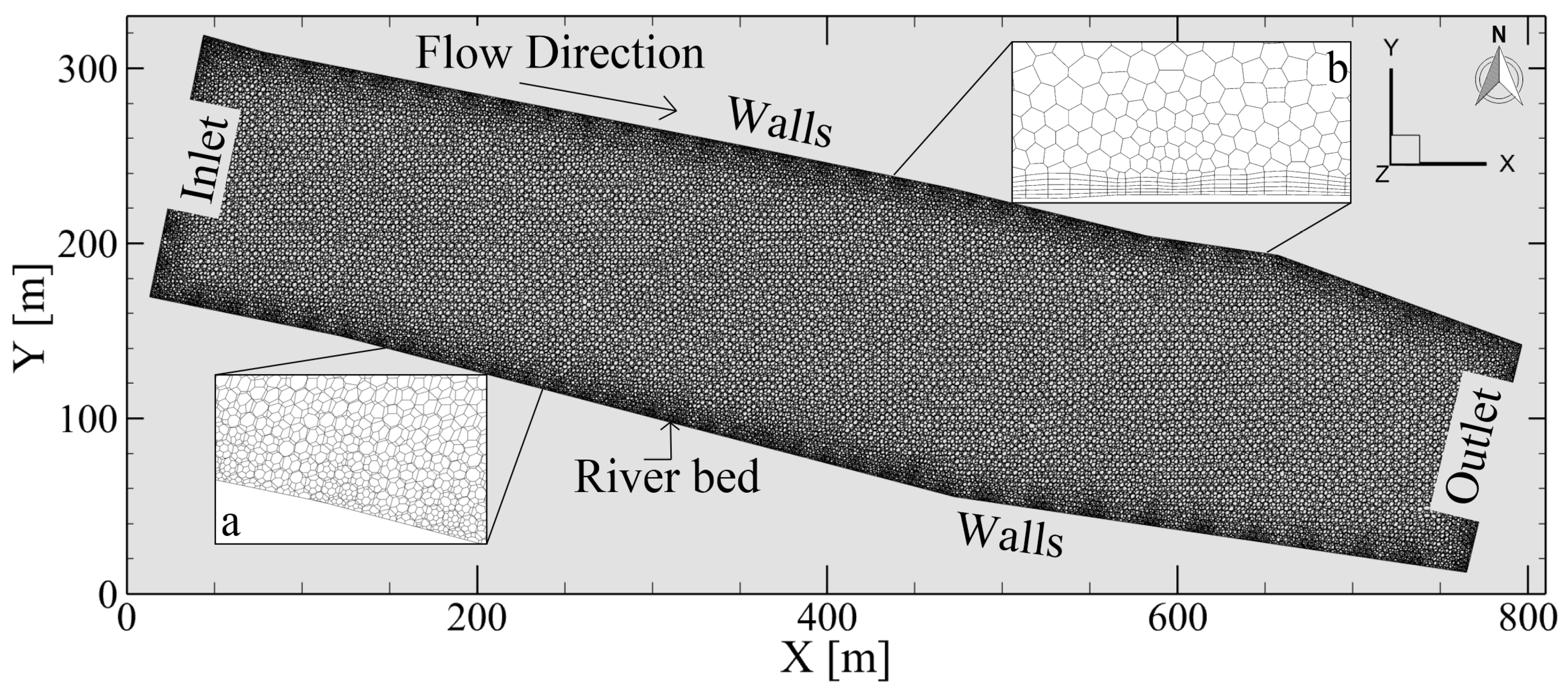
The computational mesh used in this study follows the hybrid strategy previously detailed in [67], which combines the advancing-front technique [76] with polyhedral meshing [77]. This approach ensures an accurate resolution of complex topographies and efficient simulation performance. Local refinement and inflation layers were applied near the riverbed and walls, with a first-layer height calibrated to achieve Y     1 and a growth rate of 5%, supporting near-wall turbulence resolution. Mesh quality metrics, namely the aspect ratio, orthogonality (0.9483), and skewness (avg. 0.0069), were rigorously controlled to ensure numerical stability and accuracy. A sensitivity analysis guided the selection of the final mesh configuration, which supports high-order discretization and accurate reproduction of storm-driven hydrodynamics.
Figure 2 provides a detailed view of the mesh architecture, showcasing the polyhedral cell configuration and inflation layers applied near the riverbed and along the lateral walls. This meshing framework supports high-order discretization schemes, which are vital for resolving spatial gradients in velocity, pressure, and turbulence variables with high accuracy. It also facilitates an accurate representation of flow structures, such as secondary currents, recirculation zones, and bed-induced turbulence. To ensure numerical accuracy, a sensitivity analysis was conducted to evaluate various mesh resolutions and turbulence models. The optimal mesh configuration, which was validated and presented elsewhere [67], was selected based on the convergence behavior, computational efficiency, and fidelity in reproducing field-observed hydrodynamic patterns.

4.2. Boundary Conditions

The inlet boundary was configured with a prescribed mass flow rate of 778,200 [kg/s], corresponding to an adjusted volumetric flow rate of 648.5 [m3/s]. This value was derived from hydrometric records during Hurricane Alberto, initially measured at 810.25 [m3/s] at the Cadereyta II station [78], and proportionally scaled to the study segment using established drainage area relationships [79].
In the numerical model a discharge of 810.25 m3/s was used as the initial flow condition at time t = 0 s, representing the onset of the hydrometeorological event associated. This boundary condition was applied at the upstream limit of the numerical model to assess the flow propagation along the river channel. A lateral boundary condition was imposed along the riverbanks using an open-channel condition modelling configuration to simulate wave-like surface oscillations representing marginal fluid agitation. The top surface of the domain was modeled as an atmospheric interface, allowing for free-surface deformation and accurate simulation of air–water interaction. At the upstream surface, a velocity inlet condition was prescribed, incorporating the velocity distribution and volumetric flow rate obtained from hydrological observations recorded during the storm event, including contributions from fluvial inflow and overland flooding. At the downstream boundary, although set to 0 [Pa] in gauge pressure to simulate open discharge, this corresponds to atmospheric conditions (absolute pressure = 101,325 [Pa] and temperature = 293.15° K), ensuring natural outflow while preventing artificial backflow or recirculation.
Fluid properties were defined for dense water conditions at 293.15° K, with a density of 1200 [kg/m3], dynamic viscosity μ of 0.002 [kg/(m·s)], and surface tension of 0.0583 [N/m]. All values align with previous observations of high-density runoff events in mountainous and urban watersheds in the region. The resulting kinematic viscosity (ν) was calculated as 1.667 × 10⁻⁶ [m2/s]. While a detailed tabulation is omitted here for brevity, the full dataset and sensitivity analysis are available in publication [67]. The domain was initialized with a quiescent air–water configuration, and the outlet condition was set to ensure atmospheric discharge without artificial backflow, thereby avoiding numerical instabilities. These settings define the initial hydrodynamic state of the system, ensuring that the model reproduces storm-driven inflow, channel confinement, atmospheric outflow, and free-surface interaction under dense-water conditions.
It is important to clarify that sediment transport processes were not modeled in this simulation. Incorporating sediment dynamics would require detailed input on sediment properties, such as particle diameter, specific gravity, and interaction forces, as well as a three-phase modeling framework to capture solid–liquid–gas interactions. Given the absence of such site-specific sedimentological data, the present work focuses exclusively on the hydrodynamic behavior of dense water flows during extreme weather events.

4.3. Governing Equations

In multiphase river flow simulations, the interface between phases is modeled using the continuity equation for the volume fraction of each phase. The general form of this equation is as follows:
ρ t + · ρ v = n S n ,
where ρ denotes the density, v the velocity vector, t time, and S = 0 under the initial assumption of no mass transfer between phases. To track the interface, air is considered the secondary phase α g , and its volume fraction is obtained by solving:
ρ g α g t + · ρ g α g v = 0 .
Since the volume fractions of the phases are related, the water fraction ( α w ) is determined using the relationship α w + α g = 1 .
The velocity field is shared across all phases, and a single momentum equation governs the system. This equation is weighted by the volume fraction of the phases:
t ρ v + · ρ v v = p + · μ v + v T + ρ g + F ,
where, ρ , v , p , μ , g and F represent the density, velocity, pressure, dynamic viscosity, gravitational acceleration, and body forces, respectively. The properties ρ and μ are computed as weighted averages of the phases:
ρ = 1 p ρ q α q
μ = 1 p μ q α q
where ρ q is the density of phase q , α q is the volume fraction of phase q , and μ q is the dynamic viscosity of phase q . This framework allows for accurate modeling of multiphase dynamics in river environments, including free-surface behavior and water-air interactions in high-energy zones.

4.4. Turbulence Models

The RLZ k ε turbulence model [50,80] enhances the standard formulation to better capture flows with strong streamline curvature, separation, and rotation. While assuming isotropic turbulence, it improves representation of near-wall and recirculating flows. In this study, RLZ serves as the benchmark based on its validated performance in similar fluvial simulations [67], providing the minimum precision standard for evaluating alternative models. This structure ensures that the present analysis is not merely a model-to-model comparison, but a sensitivity assessment relative to a turbulence model whose accuracy was previously established through field validation. While its computational cost is higher than the standard k ε , it remains a reliable and robust reference for large-scale riverine simulations. The next Table 1 summarizes the turbulent models’ equations an in Table 2, the parameters and constants.
Despite sharing some default parameter values with the well-established k ω SST model, GEKO features an extended formulation with tunable coefficients that improve its adaptability and performance. The default settings were applied without calibration due to the stochastic nature of the natural flood event studied, ensuring an unbiased comparison of the models under realistic hydrodynamic conditions. While default parameters are often sufficient in many cases, GEKO’s design offers greater flexibility across various flow regimes, positioning it as a versatile, unified alternative to the fragmented landscape of existing RANS models.
The BSL-EARSM model is based on the two-equation baseline (BSL) turbulence model developed by Menter, which blends the advantages of the k ω and k ε formulations through a blending function approach. It enhances the BSL model by introducing an explicit algebraic Reynolds stress model (EARSM) for the anisotropy tensor a i j , allowing for anisotropic turbulence effects without solving full transport equations for the Reynolds stresses. This is especially beneficial for flows with strong streamline curvature, secondary motions, or normal stress imbalances (common in riverine and open channel applications).
To incorporate anisotropy, the Reynolds stress tensor is written in terms of the anisotropy tensor R i j = 2 κ α i j + 1 3 δ i j . The anisotropy tensor a i j is obtained from the explicit algebraic closure, derived by assuming equilibrium between the production and dissipation of Reynolds stresses. The closure results in a non-linear expression involving the strain rate tensor S i j and rotation rate tensor Ω i j , α i j = n = 1 10 α n T i j ( n ) , where the T i j ( n ) tensor are constructed from invariant of S i j and Ω i j :and the coefficient α n are functions of the non-dimensional strain and rotation rates, typically involving the turbulent Reynolds number and ratios of second- and third-order tensor invariants.
The first few basis tensors are:
  • T i j ( 1 ) = S i j ,
  • T i j 2 = S i k Ω k j Ω i k S k j ,
  • T i j 3 = S i k S k j 1 3 δ i j S m n S n m ,
  • and so on.
This approach allows the model to capture secondary flow effects and anisotropic turbulence structures without the computational cost of solving the full Reynolds stress transport equations. This model has shown improved performance in flows with high curvature, strong adverse pressure gradients, or separated regions, conditions that frequently appear in complex riverine geometries, bridge piers, and vegetated channels.

4.5. Spatial and Temporal Discretization Strategy

To ensure methodological continuity and accuracy in representing complex hydrodynamics, the numerical framework adopted in this study builds upon our previously validated approach in [67], which employed the same computational domain, boundary conditions, and numerical schemes for the same case study. This allows direct comparison between traditional and advanced turbulence closures under identical simulation settings. The simulations employed third-order spatial discretization frameworks, including the third-order Monotonic Upstream-Centered Scheme for Conservation Laws (MUSCL) [81] for momentum, and the Resolution Interface Capturing (HRIC) scheme [82,83] for interface reconstruction, within a VoF scheme suitable for capturing free-surface dynamics. Pressure-velocity coupling was handled using the PRESTO! (Pressure Staggering Option) scheme [84] and the Pressure-Implicit with Splitting of Operators (PISO) algorithm [85,86] at different stages, ensuring numerical stability and convergence. These schemes were applied during the steady-state verification phase to confirm convergence and flow stabilization; once a quasi-steady solution was achieved, the algorithm was switched to PISO for unsteady simulations under the URANS framework.
An adaptive time-stepping strategy was implemented to resolve transient flow behaviors, with time steps ranging from 1 × 10 2 < t < 2.5 × 10 2 [67] The VoF scheme [87], which models immiscible multiphase flows with a free surface, tracks the water–air interface while ensuring phase consistency via volume-fraction constraints. The scheme uses the Continuous Surface Force (CSF) method [88] to model surface tension, improving pressure gradients near complex geometries. This refinement was crucial for capturing hydraulic features like vortex shedding, flow separation, and interactions with topography [40,89].

4.6. Mesh Independence and Validation Against Observed Flow Patterns

To ensure the reliability of the numerical results, a mesh independence analysis was conducted alongside a validation procedure based on velocity observations. Simulations were performed using ANSYS Fluent 2024 R1 [59] on a high-performance computing platform equipped with an AMD Ryzen Threadripper 3990X (64 cores), complemented by dual GPU acceleration (NVIDIA Quadro 6000 and Tesla C2075). This configuration facilitated efficient processing of large-scale, three-dimensional two-phase (air-water) simulations representative of complex riverine dynamics.
In general, the video footage used in this study was incidentally captured by news reporters during the storm event [90,91,92]. A key objective was to estimate river velocities—particularly inlet velocity—using one selected video processed with the scientifically validated software ANDROMEDE (ANDROMEDE v2206) [71], which enables accurate flow velocity analysis in natural channels. High-resolution sections of the footage were analyzed to extract velocity profiles at selected cross-sections. The measured velocities ranged from a mean of 4.4305 [m/s] to a maximum of 8.6602 [m/s]. These values were used to validate the computational model through direct comparison with simulation results. The velocities were obtained directly from the numerical output of the ANDROMEDE software, which determines flow speed through pixel displacement analysis. This method inherently limits precision to the scale resolution of the video and the accuracy of spatial calibration; therefore, all reported values have been rounded to four significant figures.
The turbulence behavior was characterized using the RLZ model, chosen for its superior performance in mesh-independence and validation studies [67]. The computational mesh was adapted to the river’s topography and 3D geometry, using techniques such as polyhedral cells, advancing-front refinement, and graded inflation layers. Mesh refinement improved accuracy, reducing velocity prediction errors significantly until a critical resolution was reached, beyond which further refinement offered diminishing returns.
The computational domain was discretized with a mesh adapted to the riverbed’s irregular geometry. Mesh configurations were evaluated based on computational time, maximum velocity, and percentage error relative to validation. Mesh refinement reduced velocity errors up to a critical resolution, with coarser meshes (≈189,000 cells) producing errors > 18%, and finer meshes (≈4.2 million cells) yielding up to 3.55% error due to numerical rounding, matrix conditioning, and over-resolution of sub-grid features.
Table 3 compiles the quantitative outcomes of the mesh sensitivity analysis, detailing the number of polyhedral cells, average simulation time, and associated velocity errors relative to observational benchmarks. This assessment was essential to determine the optimal mesh resolution for accurately capturing flow dynamics while maintaining computational efficiency.
The most accurate and computationally efficient configuration was Mesh 3, composed of 591,379 polyhedral cells. It yielded maximum and mean velocity errors of just 0.69% and 0.9%, respectively, with a computational cost of approximately 12 h per simulation. Owing to its optimal balance between accuracy and simulation time, Mesh 3 was selected for use in all turbulence model comparisons. Detailed metrics are provided in [67].
The comparison between video-derived velocity data and numerical simulations revealed critical insights into real-world flow behavior. The footage showed sections of the riverbed that were either partially submerged or obstructed by overgrown vegetation [93] prior to the storm event, with visible contrasts between areas of full inundation and partial flooding. These spatial patterns were consistently reproduced in the simulation results: the liquid-phase iso-surface closely matched field observations, and the identified flow structures remained spatially aligned with their counterparts in the experimental data. This validates the model’s ability to capture the geometric and hydraulic influence of the riverbed.
Given this agreement, Mesh 3 was adopted as the standard discretization for all subsequent turbulence model comparisons. Its validated performance [67] ensures accurate representation of near-wall flows, secondary currents, and free-surface deformation at a reasonable computational cost. All RANS closures, RNG k ε , k ω SST, k ω GEKO, and the k ω BSL–EARSM were executed under identical numerical conditions. This procedure confirms that the established mathematical model was rigorously verified through convergence checks, mesh independence analysis, and validation against field-derived velocity data, ensuring its reliability under the studied storm conditions. Simulation runtimes ranged narrowly, with RLZ completing in approximately 10 h. Table 4 summarizes the results.
The GEKO model was run without empirical tuning due to the stochastic nature of the storm, although its full potential is realized when calibrated with empirical data. The BSL–EARSM model, while more computationally demanding due to its anisotropic treatment (matrix inversions and strain rate tensor evaluations), provides superior accuracy in predicting directional turbulence effects. All models were benchmarked against the validated RLZ closure [50,67], with error indices computed to assess whether the added model complexity results in measurable accuracy improvements.
This systematic increase in computational cost parallels the growing mathematical complexity of each closure, with the EARSM’s explicit Reynolds-stress algebra and tensor operations accounting for its higher runtime. With the computational setup fully validated and the benchmark established, Section 5 presents the hydrodynamic results obtained for each turbulence model, emphasizing their performance in replicating observed flow dynamics.

5. Results and Discussion

5.1. Mean Velocity

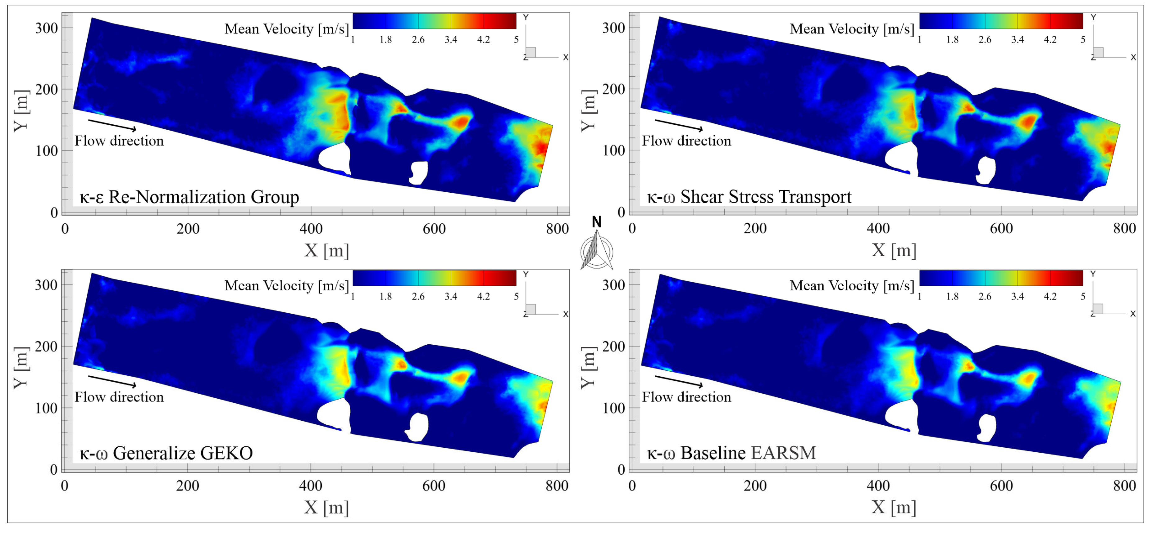
The instantaneous or mean velocities ( u i ) are derived from the Navier–Stokes solution and form the basis for all spatial derivatives. Figure 3 displays the mean velocity contours along the river channel, highlighting regions of high and low speed. Although the overall patterns are similar across models, meaningful differences emerge due to each model’s distinct formulation, which affects both accuracy and flow behavior. The empirical average velocity was 4.4305 [m/s], whereas the RLZ model (benchmark) yielded a value of 4.45 [m/s], the closest yet estimated up to that time [67]. For this reason, it is necessary to compare the results of the subsequent models against this reference.
The computed mean velocities from all turbulence models closely approximate the empirical value. The RNG model yielded a mean velocity of 4.401 [m/s]; the SST model, 4.383 [m/s]; the GEKO model, 4.412 [m/s]; and the BSL–EARSM model, 4.435 [m/s], all within a 95% confidence interval [94,95,96,97,98]. Nonetheless, the analysis of velocity iso-surfaces revealed that the location of maximum velocity differs between models, with each exhibiting focalized regions. The RNG model exhibits notably lower minimum velocities and higher maximum values than the other models, clustering low-speed regions and accentuating high-speed zones, which produces sharper gradients. This behavior mirrors empirical measurements, indicating that RNG effectively concentrates extreme values within a representative range, capturing essential features of the flow structure.
In contrast, the SST and GEKO models exhibited very similar spatial distributions of low- and high-velocity regions. Using standard constants, the GEKO model provides acceptable results and offers a clear path to improvement when measurable empirical data are available for tuning. From this standpoint, the GEKO model is more efficient under controlled experimental conditions, though even in uncontrolled scenarios such as the present case study, it still produces results that are well aligned with empirical observations.
For the BSL–EARSM model, low-velocity values are more consistent and closely match the observed speeds from video recordings [67]. This reflects the anisotropic formulation’s ability to enhance overall flow-field resolution, outperforming the more estimative predictions of the other models. Consequently, regions with currents and wave-like structures are represented more accurately than in the alternative models.
Figure 4 shows the mean velocity profiles along the central line of the computational domain, providing visual validation of the previous observations. Accurate reproduction in all three spatial directions is crucial, as over- or underestimation may indicate imbalances in turbulent production or dissipation.
Regarding velocity prediction, BSL–EARSM shows the closest agreement with the empirical mean, yielding 4.435 m/s versus 4.431 m/s, corresponding to a 0.1% relative deviation or 99% accuracy. Despite this, it underestimates low-velocity regions and has limitations in localizing high-velocity areas. GEKO ranks second with 98.58% agreement, offering a more balanced quantitative and qualitative performance, though further calibration would be needed for improved precision in real-world mesoscale applications.
The SST model achieves 98.92% accuracy but shows qualitative bias, overestimating high-velocity regions while compensating in low-velocity zones. RNG reaches 99.3% quantitatively but fails qualitatively, substantially overestimating high-speed areas and underestimating low-speed regions.

5.2. Turbulent Viscosity

Figure 5 shows the contours of turbulent viscosity, μ t , a key parameter for assessing each model’s representation of momentum transport. μ t quantifies turbulence-induced momentum transfer; excessively high values cause artificial diffusion and attenuate flow gradients, while values that are too low fail to capture unresolved turbulent structures.
Although fluid viscosity ( μ ) depends on molecular properties, temperature, and pressure, river water’s dynamic viscosity remains relatively constant. However, it may be altered by suspended sediments and entrained materials resulting from the river’s own motion and morphology. Sediment transport is excluded to isolate each turbulence model’s intrinsic performance. It is important to note that μ t are distributed over an iso-surface to illustrate development across the computational domain; minimum, maximum, and average values do not capture the full spatial distribution, representing only a portion of the overall field. This ensures correct interpretation of the model predictions without misleading assumptions about the flow.
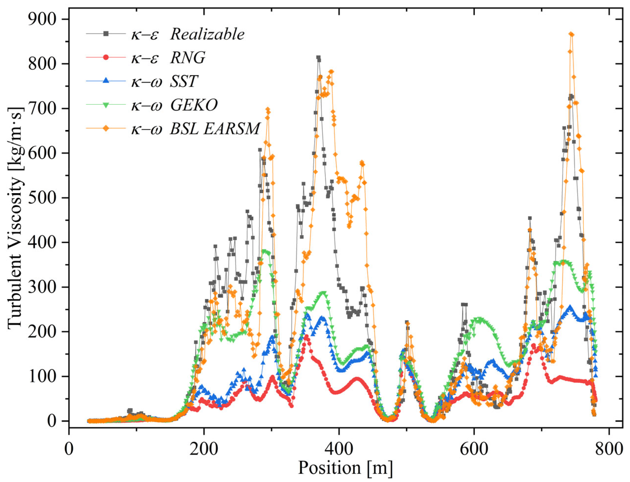
The improvements of the RNG and RLZ models enable a more accurate representation of small-scale eddies and flows with strong deformation gradients. In the river, cresting and wave-like structures develop and eventually break down. In these regions, RNG predicts μ t values ranging from 5 to 10 [kg/(m·s)], with an average of 54.8 [kg/(m·s)] and a maximum of 190 [kg/(m·s)], indicating substantial underestimation of turbulent viscosity in such zones (Figure 6 graph).
The SST model employs a blending strategy that combines the k ω model near the wall with the k ε model in the core flow region. Its turbulent viscosity ν t = k ω , includes a shear stress limiter that prevents excessive viscosity production in separated flow. This improves predictions in recirculation and flow separation, but the model tends to underestimate dynamics across the flow, particularly in breaking wave-like structures, and its isotropic formulation may introduce numerical errors. Quantitatively, SST captures similar flow zones as RLZ but predicts lower values, where μ t ranges between 25 and 26 [kg/(m·s)], with a mean of 186.5 [kg/(m·s)] and a maximum of 815 [kg/(m·s)], computed as μ t = ρ ν t where ρ is the local fluid density.
In this study, the elevated μ t values result from the combined effect of a high-density fluid, representing sediment-laden stormwater, and intense local turbulence induced by complex bed topography and wave breaking, conditions typical of extreme flood events. Although high, RLZ values are plausible under intense turbulence. In contrast, SST predicts 5 to 15 [kg/(m·s)], up to 75% lower than RLZ, with a mean of 96 [kg/(m·s)] and a maximum of 255.5 [kg/(m·s)]. Both models capture the “speckled” pattern of crests and undulations induced by flow interactions [99,100]. However, their underestimation of μ t in critical zones indicates that RNG and SST may not be suitable for accurately reproducing variable flow structures and riverine development.
The GEKO model, based on the k ω formulation, introduces adjustable functions that modify the production and dissipation terms, so that ν t = f 1 P , ε k 2 ε . f 1 is an adjustment function that depends on the production P and the dissipation rate ε . This flexibility allows adaption to various scenarios. Its values range from 15 to 24 [kg/(m·s)], an average of 145.85 [kg/(m·s)], and with maximum value reaching 381.8 [kg/(m·s)]. These values are approximately 66% lower than those obtained with the RLZ model. This model consistently represents high and low μ t regions, and the overall flow representation. However, it is unable to represent the “speckled” pattern of crests and undulations tending to homogenize the turbulent behavior.
The BSL–EARSM model combines a k ω approach with an algebraic closure for the Reynolds stress tensor, directly estimating the anisotropic tensor a i j from the velocity invariants. This captures anisotropic flows, including non-equivalent normal stresses and secondary currents, and eliminates the need for an isotropic eddy-viscosity hypothesis. μ t values range from 20 to 25 [kg/(m·s)], with a mean of 191 [kg/(m·s)] and a maximum of 867.3 [kg/(m·s)], about 6% higher than RLZ. Both BSL–EARSM and RLZ strongly display the speckled pattern of crests and waves, suggesting RLZ approaches the maximum μ t values observed in these regions.
The most comprehensive model is BSL–EARSM, followed by the highly flexible GEKO, the robust SST, and lastly RNG, which, despite improvements over the traditional k–ε model, remains limited in capturing anisotropic behaviors.

5.3. Strain Rate

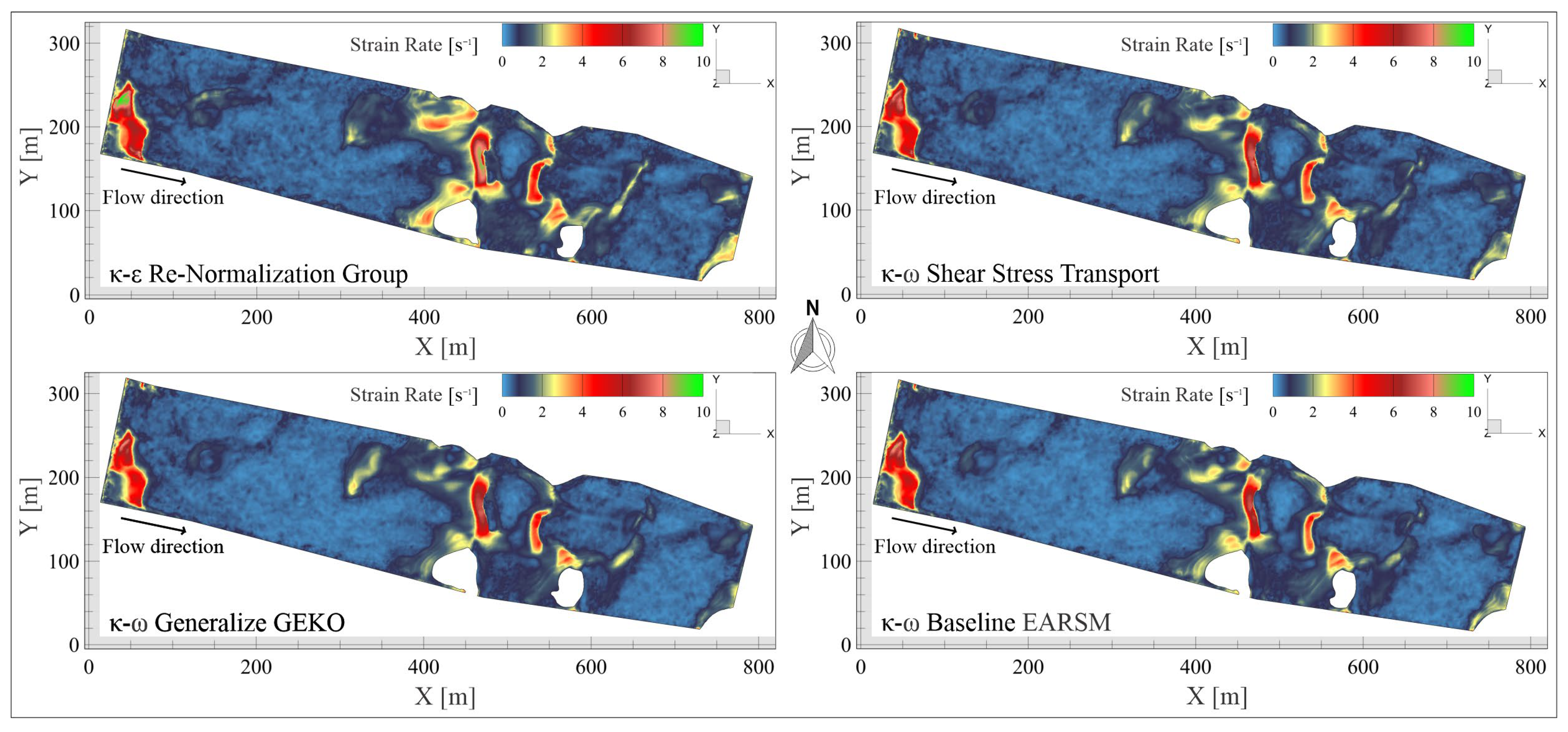
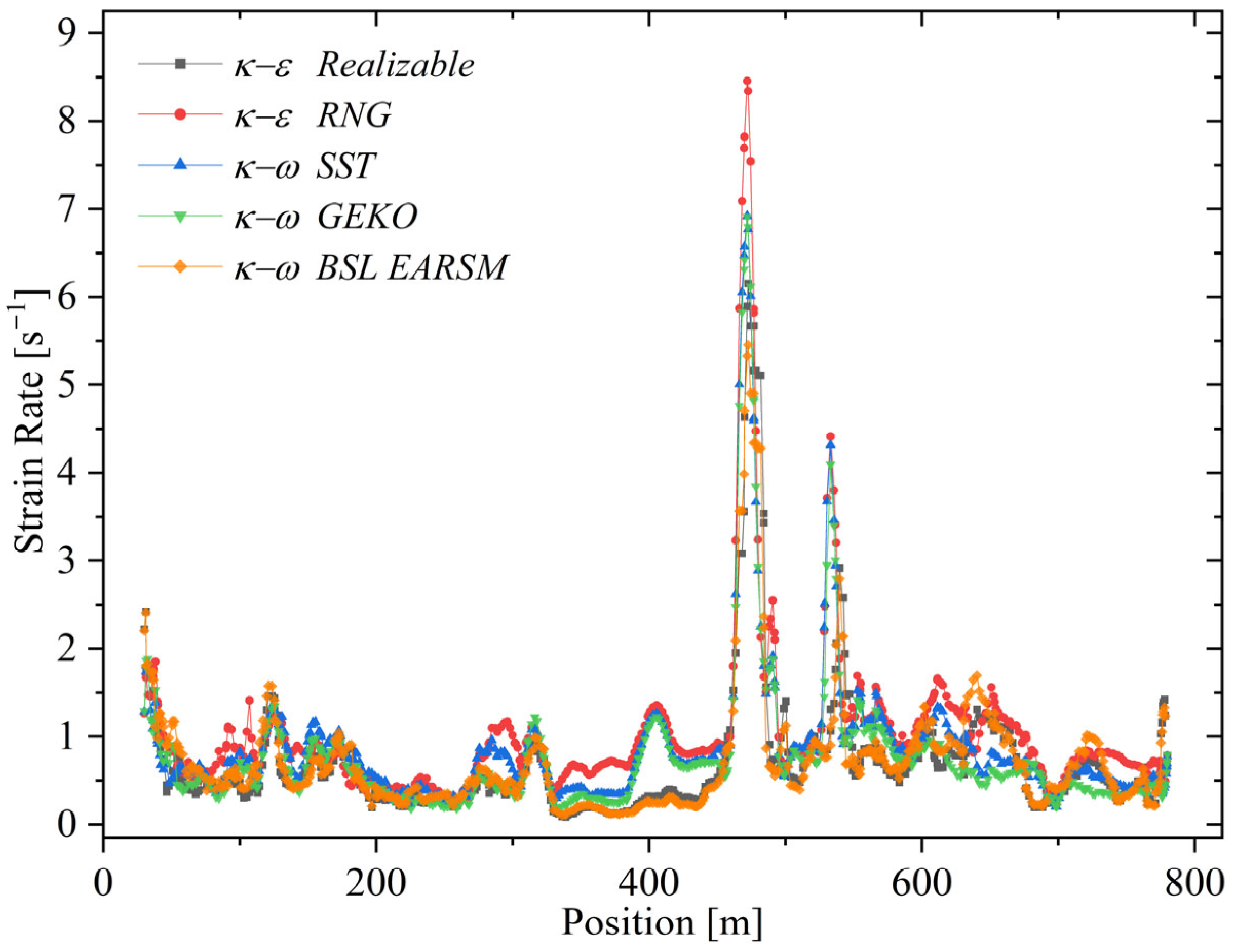
Using the RLZ model, the strain rate ranges between 0.12 and 9.0 [s−1]. The other four models display variations that highlight their relative ability to capture flow deformation gradients, as shown in Figure 7.
The SST model exhibits the highest maximum strain rate (10.27 [s−1]), surpassing RLZ, highlighting its sensitivity to intense deformation regions such as recirculation zones or near boundaries. While advantageous in high-shear areas, this may lead to overestimation if not physically justified. The GEKO model reaches 9.64 [s−1] with a minimum of 0.14 [s−1], showing a response slightly less intense than SST.
The BSL–EARSM model exhibits the lowest maximum strain rate (8.79 [s−1]) among the four models, sharing the RLZ minimum value (0.12 [s−1]). Its lower peak smooths intense deformation regions, promoting numerical stability and physical realism. However, as a second-order closure reconstructing the Reynolds stress tensor, it accurately represents turbulence anisotropy; thus, the lower maximum reflects a physically faithful response rather than a deficiency.
Figure 8 presents the strain rate along the longitudinal axis for all five turbulence models, including RLZ. All models follow a similar trend, with low-frequency oscillations from 0 to 350 [m], a sharp amplification between 400 and 600 [m], and a return to a steady baseline, reflecting recurring flow phenomena such as shear-layer growth, vortical structures, or recirculation zones consistently captured across the models.
Further analysis indicates that the RNG and RLZ predict the highest strain rates peaks near 450 and 500 [m], exceeding 8 [s−1]. heir sensitivity to rapid strain or turbulence anisotropy stems from RNG’s enhanced turbulent viscosity formulation and RLZ’s variable C μ and improved dissipation equation. This improves resolution in regions dominated by mean strain and rotation but may cause overprediction in localized shear zones, risking nonphysical gradients or numerical instability.
In contrast, the k ω (SST, GEKO, BSL–EARSM) produces smoother, damped strain rate profiles. SST achieves moderate peak resolution without abrupt spikes, while BSL–EARSM exhibits slightly lower peaks yet preserves structural coherence, likely due to enhanced stress–strain alignment.
Despite differences in peak magnitudes, all models preserve the qualitative flow structure, capturing the dominant physical mechanisms. The main divergence lies in the amplitude and sharpness of local gradients, which is critical for applications such as flame stabilization [101,102], vortex breakdown [103], or acoustic feedback [104], where accurate strain rate resolution governs mixing, efficiency, and instabilities. Underprediction may lead to insufficient mixing, whereas overprediction can artificially enhance turbulence, distorting simulation accuracy.
k ε are highly sensitive to local gradients, while k ω variants (GEKO and BSL–EARSM) provide smoother, more consistent predictions. GEKO is balanced, but BSL–EARSM stands out, closely matching the RLZ benchmark and capturing strain dynamics with high fidelity, ensuring realism and numerical stability.

5.4. Swirl Intensity

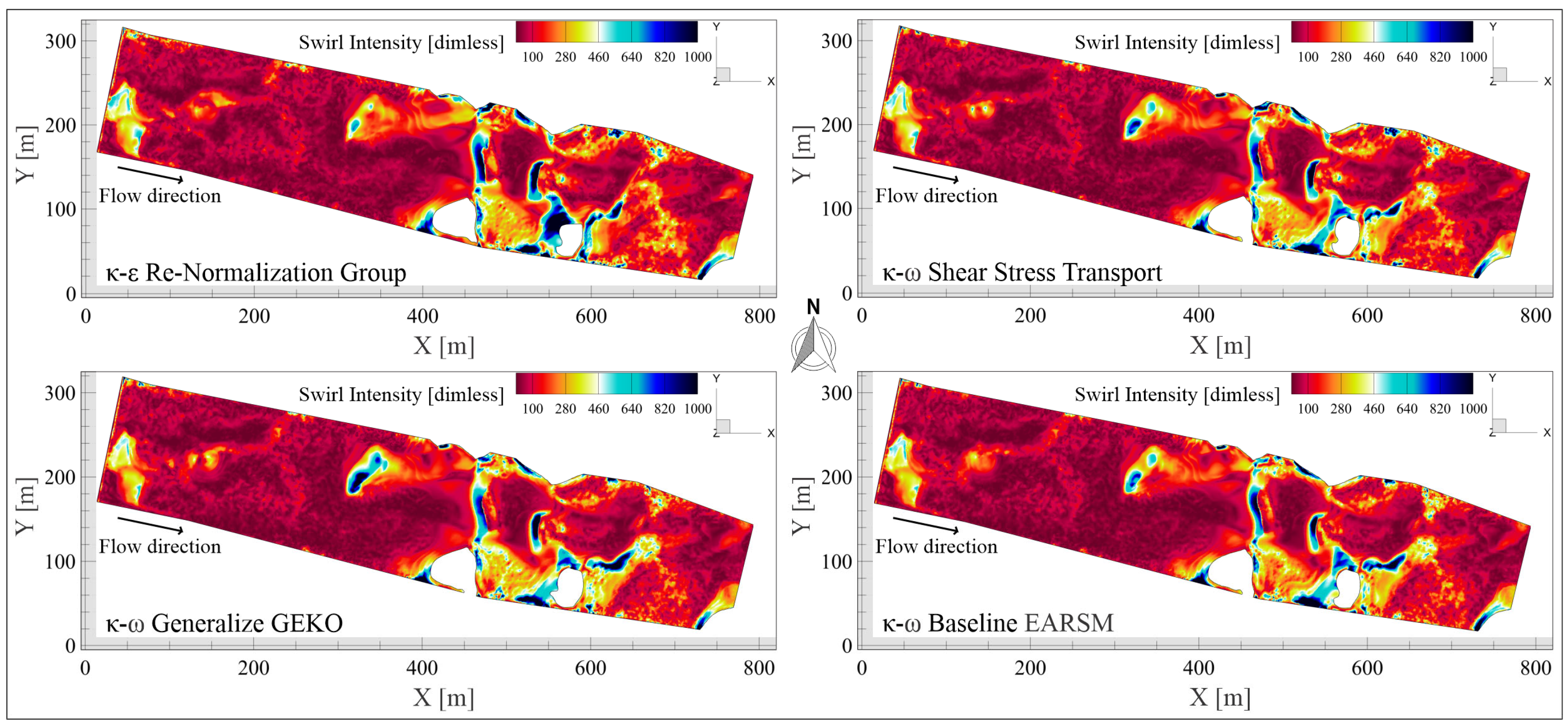
Swirl intensity, a dimensionless measure of flow rotation relative to the main axis defined as the ratio of tangential (RMS or effective) to mean axial velocity, is shown in Figure 9. The contours highlight zones of rotational dominance, helicoidal structures, and recirculation cores where tangential velocity prevails. Using the RLZ model as reference (range 12.09–1130.64, mean 152.22), it serves as a benchmark for its moderate sensitivity to rotational structures and its ability to capture mid-level vortices while limiting numerical noise, providing a robust standard for comparison.
The RNG model spans 11.86–2411.87 with a mean of 216.45, exceeding RLZ. This indicates greater sensitivity to rotational features, amplifying strong swirl regions but at the risk of added variability that demands cautious interpretation.
The SST model spans 13.9–2199.82 with a mean of 193.4, the highest minimum among all models. This implies persistent detection of rotation, enhancing vortex resolution in curved or separated flows, but also a tendency to overestimate swirl in quiescent regions.
The GEKO model spans 12.12–2184 with a mean of 172.65. It balances detection of low-swirl and intense vortices, offering adaptable sensitivity. Its tunable nature improves targeting of swirl-dominated regions while avoiding uniform overestimation, enhancing physical consistency in complex flows.
The BSL–EARSM model spans 7.78–977 with a mean of 150.85, the narrowest range among all cases. Its Reynolds stress formulation enables selective swirl resolution in anisotropic regions, yielding conservative amplification that enhances reliability in complex geometries while limiting extreme swirl capture.
Figure 10 illustrates the axial evolution of swirl intensity. All turbulence models exhibit consistent behavior in the low-intensity regime (up to ~150 m), indicating that in the developing entrance region, where swirl generation mechanisms remain weak, model formulation exerts minimal influence on the predicted dynamics. However, downstream of 150 [m], the SST and GEKO models exhibit sharper peaks and higher fluctuations, reflecting sensitivity to strong velocity and vorticity gradients, such as vortex breakdown or shear-layer instabilities. Around 530 [m], both predict the global maximum swirl intensity. The SST model responds strongly to boundary layer separations and swirling structures, while GEKO flexibly adapts to local flow conditions, capturing localized vortex stretching and anisotropic turbulence.
In contrast, the RNG and RLZ models exhibit smoother, more conservative swirl intensity profiles while capturing the overall flow structure. Their damping reflects the isotropic eddy-viscosity assumption and Boussinesq limitations. The RLZ model’s modified turbulent viscosity and alternative dissipation equation enhance rotation and strain response but remain less sensitive to localized swirl peaks. The RNG model, with differential dissipation and high-strain adjustments, responds slightly more than RLZ but does not reach the peak magnitudes of k ω -based models.
The BSL–EARSM model exhibits smooth, controlled swirl intensity throughout the domain by replacing the linear eddy-viscosity assumption with nonlinear relations between the Reynolds stress tensor and mean strain and rotation tensors. While this produces comparatively damped peaks, it likely reflects a more diffused treatment of coherent structures and greater numerical robustness, trading maximum intensity for reliable predictions of integral quantities such as torque, pressure drop, or mixing rate.
Among the models, SST and GEKO exhibit high sensitivity to sharp gradients and vortical structures with GEKO balancing vortex resolution and low numerical noise, while SST may slightly overestimate rotation. Conversely, the k ε family produces smoother, conservative predictions suitable for global flow analysis but less responsive to localized peaks. RNG amplifies swirl intensity but risks overprediction, whereas BSL–EARSM offers stable, physically consistent results with damped extreme swirls. Model selection therefore balances localized fidelity, numerical robustness, and application sensitivity.

5.5. Shear Stress

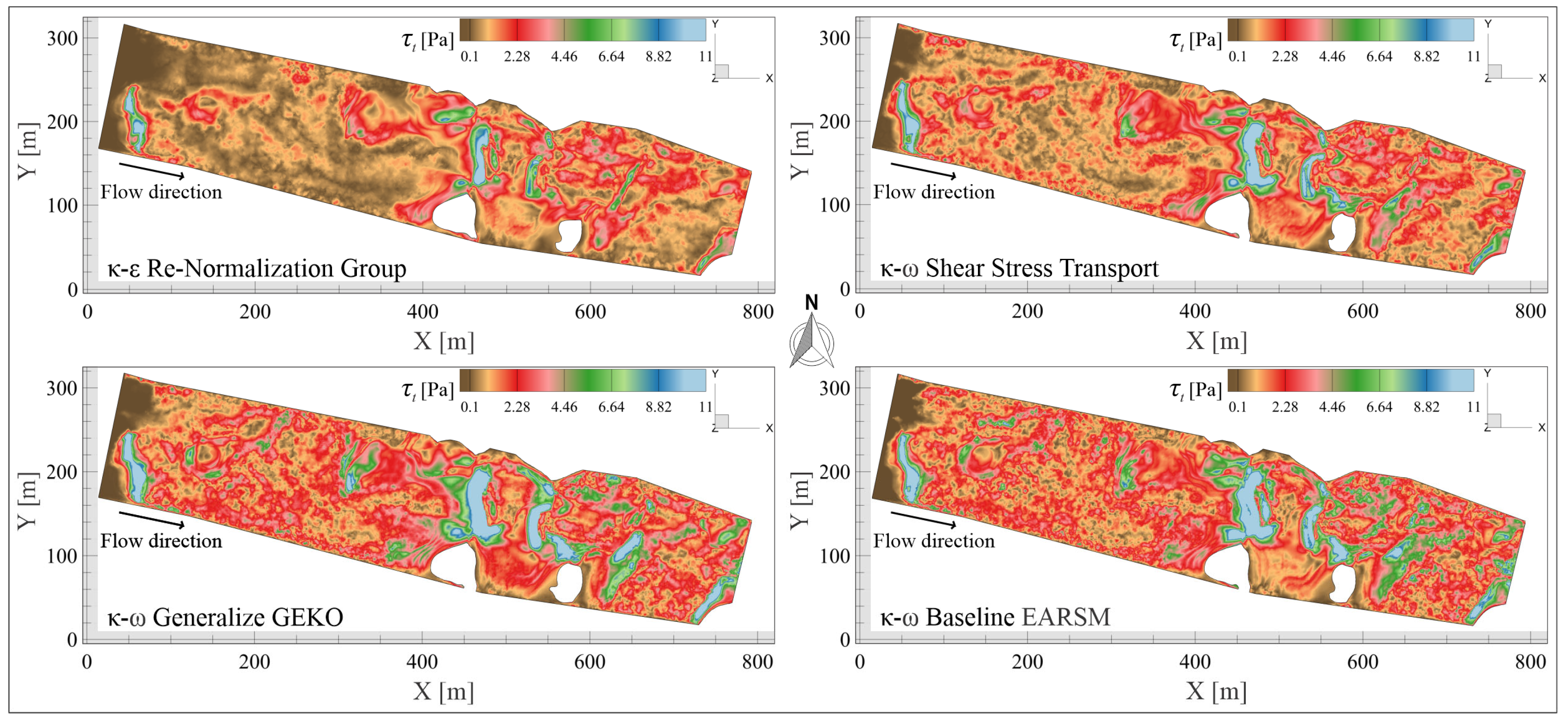
Shear stress, τ , is a key variable in riverine flow, describing how flow energy is transferred to the bed and channel walls, influencing hydraulic resistance, secondary turbulence, and sediment mobilization. Evaluating τ with different turbulence models helps assess flow intensity and understand the flow’s interaction with channel topography, obstructions, and bed irregularities (see Figure 11).
Each turbulence model produces a unique stress distribution, reflecting its assumptions and formulations, particularly in terms of turbulent mixing, momentum diffusion, and stress anisotropy. To illustrate these differences, two formulations of shear stress are considered: turbulent shear stress ( τ t ) and hydraulic shear stress ( τ h y d r o ).
τ t , calculated from ν t and vertical velocity gradients, and vertical velocity gradients, reflects the flow’s local response to riverbed perturbations. It is governed by turbulent momentum diffusion, influenced by bed roughness, channel geometry, and the flow’s three-dimensional complexity. This stress is particularly elevated near obstacles like piers or boulders, and its accuracy depends on the turbulence model used.
The key difference between τ t and τ h y d r o is their interpretation: τ t quantifies the local momentum transfer due to turbulence, sensitive to model characteristics and geometry, while τ h y d r o represents flow-bed friction from the mean flow behavior. τ t is useful for detecting erosion or vortex zones, while τ h y d r o helps assess particle motion thresholds and channel bed stability.
The GEKO model, with the highest τ t values stand at capturing high-energy dissipation regions, such as recirculation or flow separation, making it effective for modeling scour hole formation or turbulence zones downstream of structures. While the SST model shows a broader range than RNG, it avoids overrepresentation of intense gradients. The BSL–EARSM model, using anisotropic Reynold’s stress, balances local accuracy with stress field coherence, making it ideal for complex geometries where anisotropy is significant.
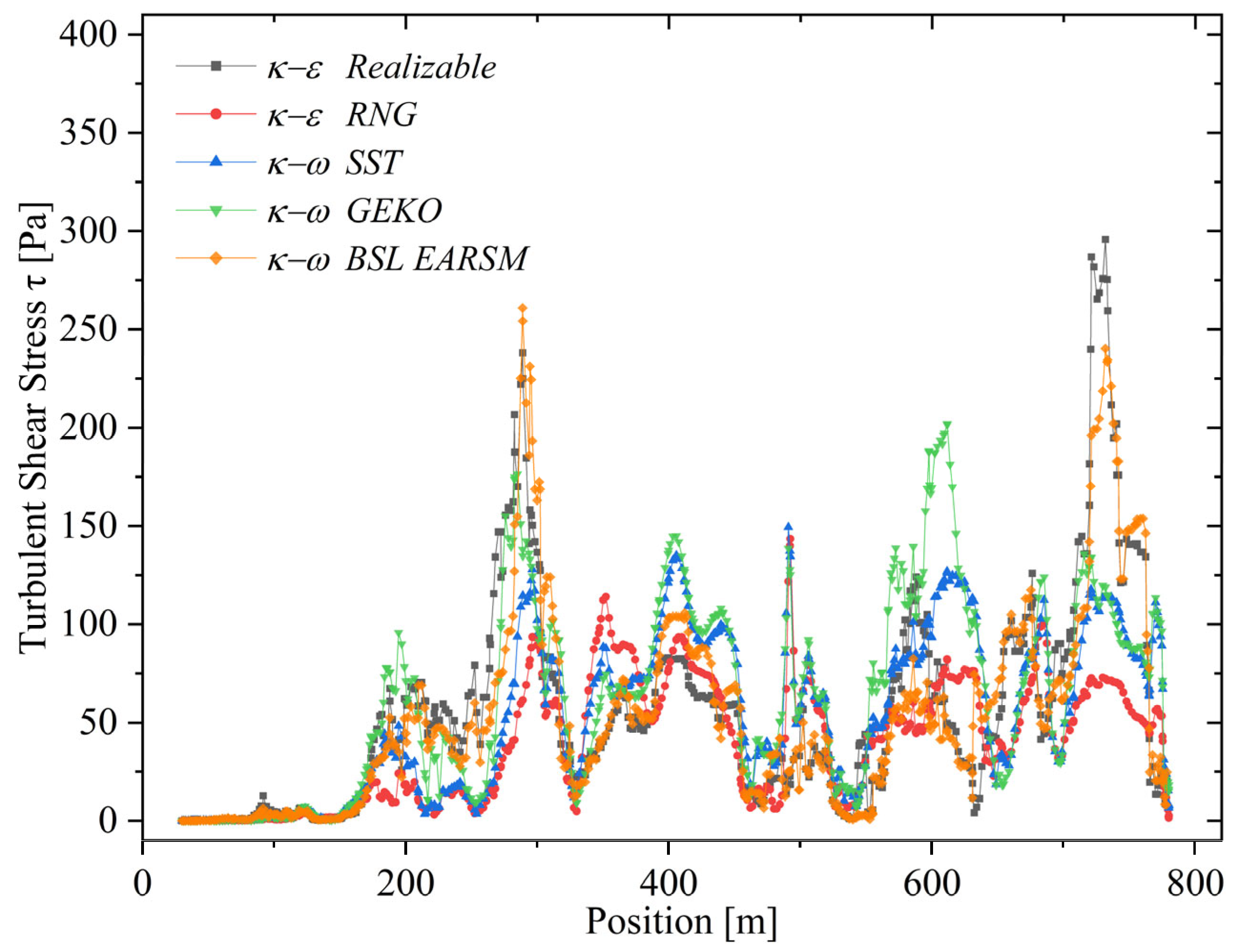
Figure 12 shows shear stress distribution along the river flow centerline for all four turbulence models. τ t values vary across models, with the RNG model reaching a maximum of 39.7 [Pa], and a mean of 2 and 6 [Pa]. The SST model shows a higher range, peaking at 51.7 [Pa] and a mean of up to 8 [Pa]. The GEKO model predicts even higher values, peaking at 66.5 [Pa] and averaging 4 and 8 [Pa], suggesting greater sensitivity to velocity gradients. The BSL–EARSM model falls in between, with a maximum of 61.5 [Pa] and a similar mean range as SST and GEKO. These variations reflect each model’s ability to capture local flow and turbulent mixing intensity.
τ t values vary across models, with the RNG model reaching a maximum of 39.7 [Pa], and a mean of 2 and 6 [Pa]. The SST model shows a higher range, peaking at 51.7 [Pa] and a mean of up to 8 [Pa]. The GEKO model predicts even higher values, peaking at 66.5 [Pa] and averaging 4 and 8 [Pa], suggesting greater sensitivity to velocity gradients. The BSL–EARSM model falls in between, with a maximum of 61.5 [Pa] and a similar mean range as SST and GEKO. These variations reflect each model’s ability to capture local flow and turbulent mixing intensity.
In contrast, hydraulic shear stress, defined as τ h y d r o = ρ · u s h 2 , represents the mean action of the flow on the channel bed, governed by the global friction mechanism. It depends on the shear velocity ( u s h ), which reflects the average near-bed velocity behavior. While not sensitive to local variations, it provides a general measure of the flow’s stress on the substrate, useful for engineering applications like erosion protection design or hydraulic structure sizing.
The RNG model predicts the highest τ h y d r o values suggesting a more energetic near-bed velocity field, possibly due to lower turbulent dissipation or greater velocity concentration in the basal zone. In contrast, BSL–EARSM yields the lowest τ h y d r o , likely due to a more uniform distribution of turbulent energy or better representation of three-dimensional flow effects that reduce bed stress. A comparative analysis of τ t and τ h y d r o across the models highlights systematic differences based on the turbulence closure used.
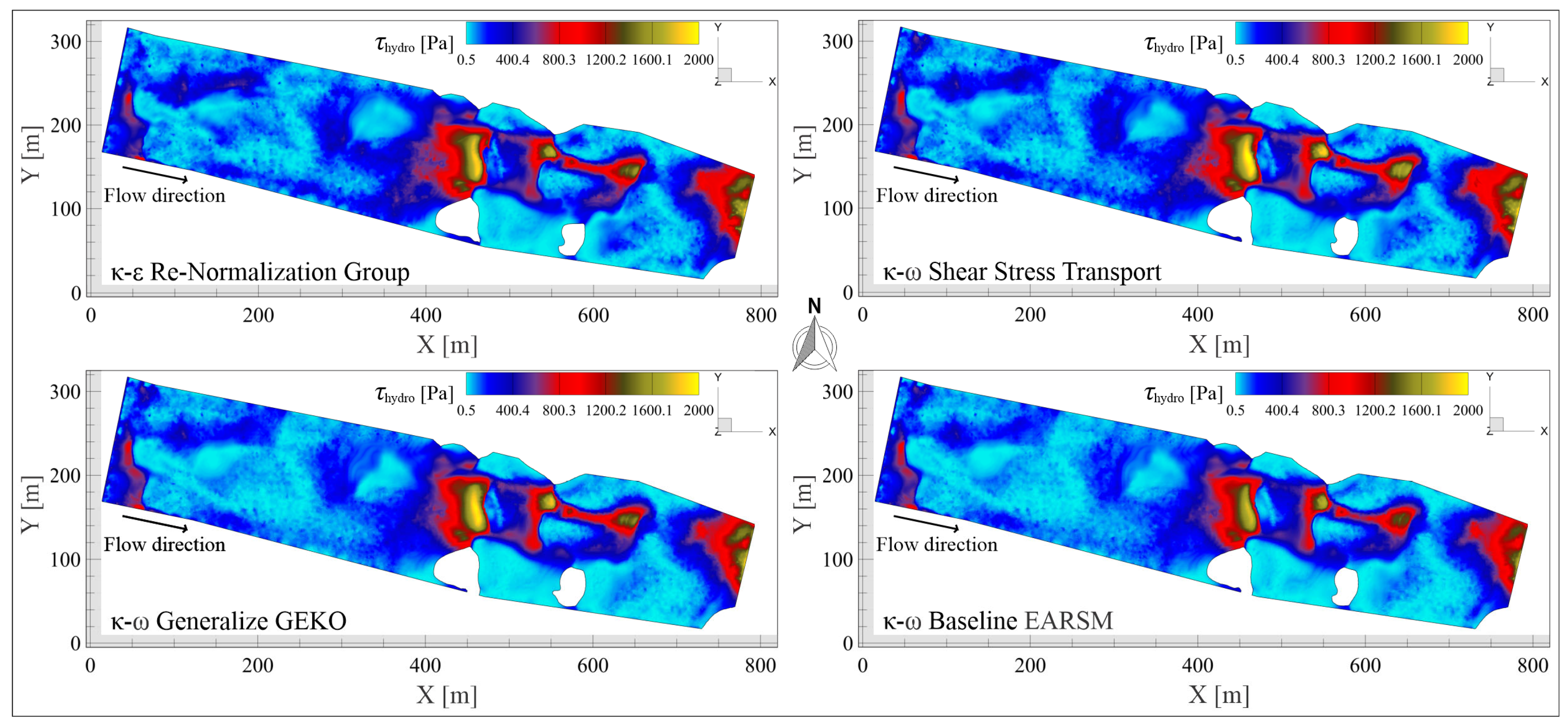
τ h y d r o values exhibit distinctly higher ranges than τ t , starting from 0.4–0.7 [Pa] and reaching peaks over 2000 [Pa] in all models. RNG yields the highest τ h y d r o (2266.19 [Pa]), followed by SST (2123.83 [Pa]), GEKO (2061.62 [Pa]), and BSL–EARSM (1934.79 [Pa]). Unlike τ , τ h y d r o is less sensitive to pointwise velocity variations and is primarily influenced by u s h , reflecting the overall hydraulic resistance. The differences in maximum values suggest that τ h y d r o is still influenced by the velocity field each model produces.
The GEKO model yields the highest local τ t , whereas RNG gives the largest τ h y d r o . SST and BSL–EARSM behave similarly, though SST produces a wider range of turbulent shear stresses. These differences are critical for applications such as erosion, sediment transport, or hydraulic resistance, highlighting that the interpretation of τ depends on the estimation method. Iso-surfaces in Figure 13 further illustrate these results.
Model performance depends on the analysis objective. For resolving local phenomena such as vortices, boundary instabilities, or erosion, GEKO and BSL–EARSM, with their higher sensitivity to τ , are preferable. For hydraulic resistance or channel-scale assessments, τ h y d r o from RNG or SST is more appropriate. These differences arise from how each model represents momentum transfer to the bed, either via local turbulent diffusion or integrated hydraulic friction, shaping the predicted stress fields. While τ reflects vertical shear from horizontal velocity gradients, τ h y d r o and u s h invert the approach, starting from an averaged stress to infer near-bed velocity. Thus, τ captures the flow’s vertical response, whereas τ h y d r o and u s h provide integrated measures of bed–flow interaction.

5.6. Shear Velocity

The u s h , in [m/s] is directly associated with the flow-induced drag over the riverbed and plays a critical role in understanding key processes such as the initiation of sediment motion, the generation of near-bed turbulence, and the development of bedforms such as ripples and dunes.
Physically, u s h represents the intensity with which the flow “carves” or “pushes” against the channel bed. Higher values of u s h indicate an increased capacity of the flow to dislodge bed particles, enhance τ , and trigger secondary vortical structures. In a lateral cross-sectional view of the river, this manifests as a steepening of the vertical velocity gradient near the bed (typically described by the logarithmic velocity profile) while in a plan view, it correlates with the formation of small-scale waves and vortices near bed roughness elements or flow obstructions.
u s h is also strongly linked to the emergence of helical flow structures: when u s h reaches sufficiently high values, it can induce transverse flow components toward the channel banks and subsequently upward toward the surface, giving rise to spiral patterns such as meander-induced vortices or those that develop around bridge piers.
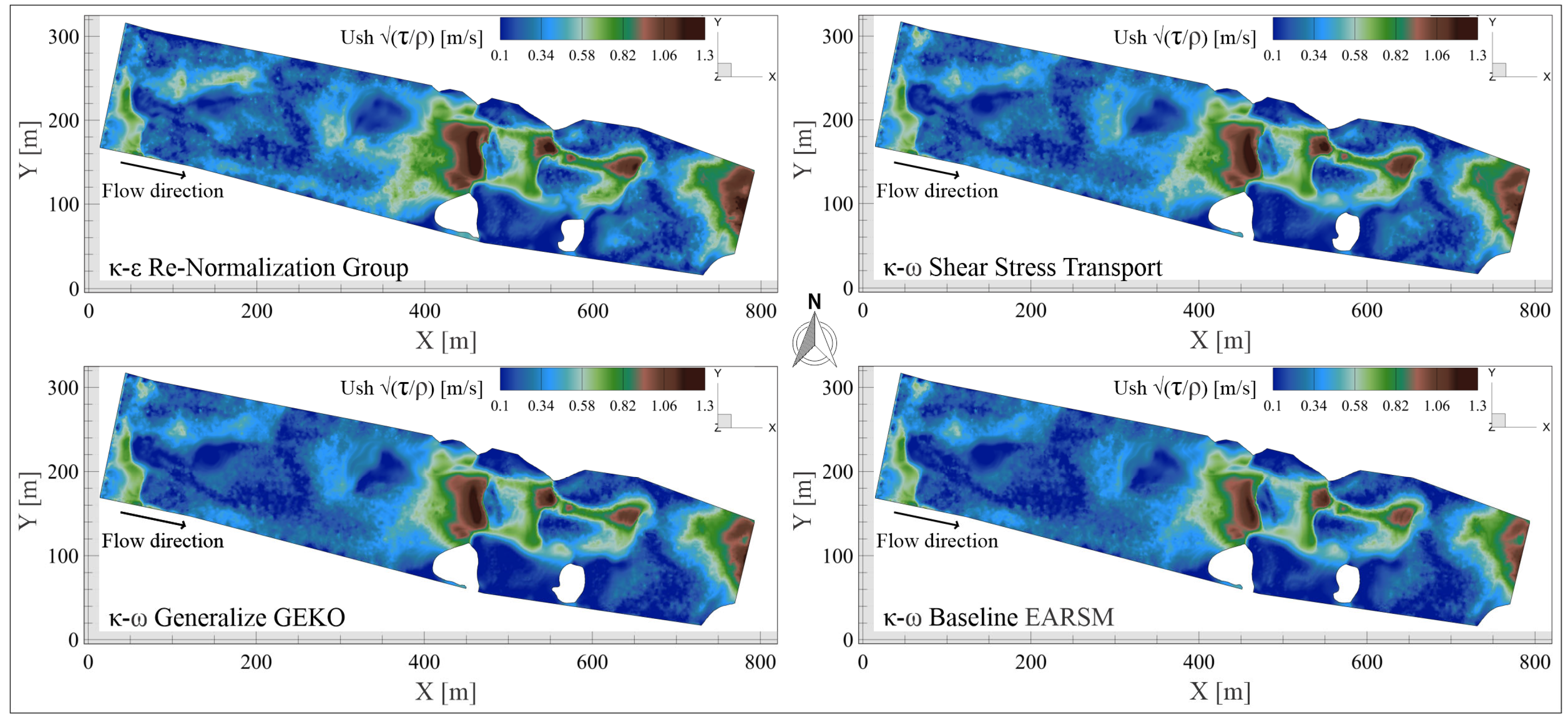
Figure 14 presents the spatial distribution of the shear velocity u s h on the iso-surface of the free surface for all four turbulence models, highlighting zones of elevated near-bed shear as well as regions where the velocity gradient is reduced due to local flow stagnation or recirculation. This visualization elucidates the variation in shear intensity and its correlation with bed interaction, flow disruptions caused by obstacles, and the formation of secondary currents.
The RNG exhibits the highest maximum value ( u s h = 1.32 [m/s]), suggesting an enhanced capability to capture regions of elevated shear stress near channel bed or vicinity of flow obstructions that intensify the velocity gradient. Its minimum value ( u s h = 0.01856 [m/s]) indicates a degree of sensitivity in low-shear regions, such as recirculation or flow shielding.
The k ω SST model shows a slightly lower maximum ( u s h = 1.278 [m/s]), accompanied by a higher minimum ( u = 0.02127 [m/s]), which may reflect a more uniform model response. This behavior supports greater numerical stability and smoother shear profiles, potentially desirable in applications where robustness is prioritized over capturing localized shear fluctuations.
The GEKO model yields the second-highest maximum value of u s h = 1.259 [m/s] and a minimum of 0.02336 [m/s], positioning it as a highly responsive yet potentially less conservative model. Its relatively elevated minimum suggests a tendency to slightly overestimate basal shear in low-activity zones. Nevertheless, its overall narrow and controlled range can be advantageous for maintaining computational stability while retaining the ability to resolve localized shear.
Finally, the BSL-EARSM model reports the lowest maximum ( u s h = 1.22 [m/s]) and minimum ( u s h = 0.0178 [m/s]) values, reflecting a more conservative approach to shear stress estimation. Given its anisotropic stress formulation, the model may inherently dampen the estimation of u s h compared to models relying on isotropic turbulence assumptions. This trait potentially enhances physical realism in complex directional flows, though it may lead to underestimation of drag forces under extreme flow conditions.
GEKO shows intermediate sensitivity, combining high peak response with stability. RNG spans the widest range, suitable for resolving shear extremes. BSL–EARSM yields smoother basal shear, while SST balances stability and gradient responsiveness, favoring moderately rough flows.

5.7. Q Criterion

The analysis of the Q-criterion is performed to identify and visualize coherent vortical structures within a three-dimensional flow field. It is particularly useful in CFD simulations, especially in applications involving complex hydrodynamics. This criterion distinguishes regions of the flow where rotation (vorticity) dominates over strain (rate of deformation), thereby enabling the detection of vortices, recirculation zones, rotational waves, and other phenomena that directly influence sediment transport or erosion.
Q is defined as a scalar: Q = 1 2 ( Ω 2 S 2 ) where: Ω is the vorticity or rotation tensor (the antisymmetric part of the velocity gradient tensor). S is the strain rate tensor (the symmetric part).
Q   >   0 : Rotation dominates → indicative of vortices or coherent vortical structures.
Q   <   0 : Strain dominates → indicative of shear or extensional flow.
Q   =   0 : Balance between rotation and strain.
In riverine flows Q > 0 near the bed or around bridge piers signals high erosion potential, while the free surface, such vortices can lead to breaking waves or circulation patterns that alter the flow direction. These regions are often associated with elevated azimuthal velocities and high levels of local turbulence.
Figure 15 presents the iso-surface contours of the Q-criterion for each turbulence model. The SST reaches the highest maximum Q = 23.0636   [ s 2 ] , suggesting superior resolution of coherent vortical structures, particularly in transitional zones between near-bed and outer flow regions. It preserves near-bed vorticity while limiting excessive dissipation, effectively capturing helicoidal vortices that rise toward the free surface (phenomena typically observed in channel bends or zones of flow expansion) and supporting representation of bottom-surface interactions, vertical angular momentum transport, and upstream-propagating internal instabilities.
Closely following SST, the GEKO model reaches a maximum Q   =   22.7463   [ s 2 ] with a less negative minimum, producing moderately intense yet spatially coherent vortices and reduced numerical diffusion. Its higher minimum Q value indicates a more favorable balance between rotation and strain, favoring vortex identification with reduced influence from linear deformation.
The BSL–EARSM model achieved a maximum Q of 21.6702 [s−2] and a minimum of 7.2123   [ s 2 ] , offering notable advantages through its explicit reconstruction of the Reynolds stress tensor. This facilitates the formation of anisotropic vortices with realistic orientation and structure, particularly in curved flows, confluences, or over naturally rough beds. Although its maximum vortex intensity is slightly lower than SST and GEKO, BSL–EARSM outperforms in generating organized and physically consistent vortical structures.
The RNG recorded the lowest maximum Q   = 19.7897   [ s 2 ] and the most negative minimum 10   [ s 2 ] , reflecting a spectrum dominated by strain. It captures both vortical zones and high-strain regions, indicative of coexisting persistent eddies and areas of strong viscous dissipation, as typical in meandering channels or near obstacles, though smaller-scale vortices may lose coherence.
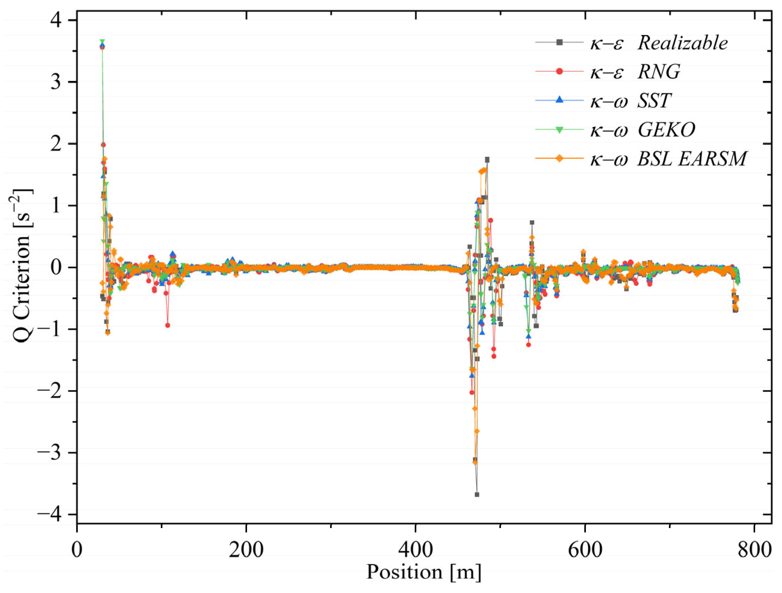
Figure 16 shows Q-criterion fields for all five turbulence models, highlighting differences in their capacity to resolve vortex intensity, coherence, and spatial organization in complex fluvial flows, despite all adequately representing rotational dynamics.
Overall, SST and GEKO capture the most intense vortical structures, followed by BSL–EARSM, while RNG is more conservative. Model choice thus depends on the desired detail and realism for representing rotational phenomena such as plunge pools, breaking waves, or helical structures. SST is particularly suitable when turbulent transport, localized erosion, or secondary flows are critical. Physically, the Q-criterion identifies regions where rotation dominates over strain: positive Q indicates coherent vortical structures, whereas negative Q highlights areas of linear deformation.
In three-dimensional river flows, positive Q values indicate eddies, helical structures, and recirculation cores, generated by pressure gradients, bed topography, wall friction, or obstacles. Local angular momentum accumulates where velocity gradients produce strong rotation, creating vortices that move vertically or laterally. These appear as streamlines curving around an axis, circular waves, depressions, or surface elevation, and may form retrograde waves or bowl-shaped structures transferring energy from bed to surface. Negative Q values mark deformation-dominated zones, where flow stretches or compresses, forming thin shear layers or strong velocity gradients, signaling transitions between attached and detached flow rather than coherent vortices.
As the maximum value of Q increases in a computational domain, it can be inferred that the turbulence model captures more intense and persistent rotational structures. These are not mere local fluctuations but rather organized motion fields that play a direct role in transporting momentum, energy, and potentially sediments. Such structures may remain anchored in specific regions or migrate depending on the balance between rotation and shear. Their existence is essential for explaining phenomena such as local scouring around bridge foundations, the formation of standing waves in contraction zones, and the vertical dispersion of contaminants or suspended particles.
From an energy perspective, the Q-criterion highlights zones where flow energy is retained as organized rotation rather than dissipated through viscous deformation. High positive Q values indicate that the flow resists stretching, forming persistent three-dimensional vortices or eddies and secondary helical structures along the channel, particularly in bends or after slope changes. These vortex cells redistribute angular momentum vertically, with inclined or vertical axes that drive fluid upward, enhance vertical mixing, and potentially lift sediments or generate hydrodynamic surface waves from three-dimensional vorticity.
The combined analysis of Q with other variables, such as τ , pressure fields, and turbulent kinetic energy, not only enables the detection of these structures but also allows the prediction of where the flow has the potential to generate vertical transport, localized erosion, or persistent wave patterns, all of which are key physical effects in real fluvial dynamics.
  • SST is the model that predicts the most intense vortices and the development of structures from the bottom toward the surface, making it the most prone to simulating internal waves and flow breaking due to vorticity accumulation.
  • GEKO is the most stable and configurable, useful when seeking to control the shape and persistence of structures without saturating the solution.
  • BSL–EARSM offers more realistic structures in terms of orientation and shape, making it ideal for physical flow analysis, especially in complex channels.
  • RNG produces broad deformation zones with distinct but somewhat more dispersed or irregular vortices, useful under transient flow conditions and hydraulic jumps.
The observed differences among the turbulence models can be directly attributed to their underlying formulations. The k − ε family models (RNG, RLZ) tend to concentrate velocity extremes and overpredict in regions of strong gradients due to their isotropy assumptions. The k–ω SST provides smoother profiles and mitigates excessive viscosity but may underestimate local structures. The GEKO introduces adjustable functions that enhance adaptability, though in the absence of calibration it tends to homogenize the turbulent field. The BSL–EARSM, by explicitly reconstructing anisotropic Reynold’s stress tensors, achieves the most accurate representation of secondary and anisotropic flows, albeit at a higher computational cost. These findings highlight that the divergence in predictions arises from differences in assumptions (isotropy vs. anisotropy), mathematical formulations (linear closure vs. explicit algebraic), and the degree of flexibility or calibration available in each turbulence model.
Nevertheless, these recommendations should be interpreted with caution. Enhanced closures such as BSL–EARSM demand higher computational resources, while models like GEKO may show sensitivity to site-specific calibration. These aspects highlight the need to balance predictive accuracy against computational feasibility and data availability in practical applications.

6. Conclusions

This study presented a detailed sensitivity assessment of enhanced 3D RANS turbulence models applied to real-world river hydraulics under extreme storm conditions. While all models predicted bulk mean velocity within 1% of the observed value, their ability to resolve key turbulent structures and anisotropy varied significantly, with implications for the accurate representation of complex riverine flows.
  • BSL–EARSM exhibits outstanding capabilities in physically describing coherent and three-dimensional flow structures. Its representation of the Q-criterion, the helical organization of streamlines, and the distribution of turbulent dissipation more realistically reflect bed-surface interactions, the development of lateral vortices, and recirculation zones. Its swirling intensity and shear velocity are physically consistent with flows dominated by separation, mixing, and secondary pulsation. This model proves to be the most suitable and optimal for representing fluvial flows with complex and anisotropy structures making it the most physically accurate closure for simulating complex flow structures in natural rivers, more realistic predictions of turbulent viscosity and strain-rate distributions, and with no higher computational cost.
  • GEKO closely follows BLS–EARSM in performance, proving to be a flexible alternative delivering robust predictions even without site-specific calibration and offering promise for applications where empirical data for tuning are unavailable. However, it tends to be slightly more conservative regarding extreme values of shear velocity and swirling intensity, and it provides high spatial coherence in regions of strong flow deformation. It is particularly useful when a balance between accuracy and computational robustness is required and in scenarios involving smooth transitions between laminar and turbulent regimes or controlled flow conditions.
  • The SST model is balanced in terms of accuracy and is computationally efficiency, effectively resolving key features like shear layers and separation zones, but exhibited a tendency to overestimate turbulent viscosity in certain high-shear regions. It produces intense but more diffuse structures in its predictions. It is ideal for identifying separation and reattachment zones, although it may overestimate turbulent kinetic energy in certain cases.
  • RNG produces less-organized structures with greater spatial dispersion, which may be useful for representing highly fluctuating turbulence but is less suitable for structured flow analyses. Nevertheless, it showed limitations in representing low-velocity and recirculation zones and tended to diffuse key turbulent structures, which are essential aspects for riverine modeling.
  • RLZ serves as a minimal reference; its low complexity ensures fast computations but renders it insufficient for capturing the complex details of riverine flows.
A detailed analysis of multiple turbulent variables, including ω i , swirling intensity, u s h , the Q-criterion intensity, and the physical structure of the flow, demonstrates that the accurate representation of riverine flow does not depend solely on the magnitude of extreme values but rather on the physical coherence of the generated turbulent structures, their alignment with field-observable phenomena (such as vortices, scour holes, and retrograde wave breaking), and the model’s ability to correctly capture the anisotropy of the flow.
Overall, these findings highlight the importance of selecting turbulence models based on the specific hydrodynamic features of interest and the balance between computational cost and physical fidelity. Enhanced models such as BSL–EARSM offer clear advantages for studies requiring accurate resolution of anisotropy and secondary flows, whereas models like GEKO provide a promising alternative when calibration is feasible or computational efficiency is prioritized.
These insights allow for a practical classification: BSL–EARSM is recommended for high-fidelity modeling where anisotropy, coherent structures, and near-wall effects are critical; GEKO serves as a reliable compromise for robust, moderately accurate predictions in data-scarce contexts; SST is suitable for balanced analyses in scenarios dominated by separation and reattachment; and RNG or RLZ are better reserved for rapid preliminary screening when physical detail is not the primary objective.
Finally, this study establishes a foundation for future research focused on integrating key dimensionless parameters, namely the critical Froude number, Reynolds number, and Shields parameter, to enhance the quantification of flow regimes, sediment transport thresholds, and hydraulic similarity in complex riverine conditions. Additionally, this study paves the way for exploring alternative formulations to model different types of shear stress (both local and integrated). It also allows for assessing their implications under flow conditions around structures such as piers and in hypothetical scenarios involving variable fluid densities, material concentrations, and compositional gradients. These extensions will contribute to establishing a more versatile and applicable methodological framework for the analysis of natural rivers and complex hydraulic systems.

Author Contributions

Conceptualization, M.D.l.C.-Á. and R.B.; methodology, M.D.l.C.-Á. and R.B.; software, M.D.l.C.-Á.; validation, M.D.l.C.-Á.; formal analysis, M.D.l.C.-Á.; investigation, M.D.l.C.-Á. and R.B.; resources, M.D.l.C.-Á. and R.B.; data curation, M.D.l.C.-Á.; writing—original draft preparation, M.D.l.C.-Á.; writing—review and editing, M.D.l.C.-Á. and R.B.; visualization, M.D.l.C.-Á.; supervision, R.B.; project administration, R.B.; funding acquisition, R.B. All authors have read and agreed to the published version of the manuscript.

Funding

This research received no external funding.

Data Availability Statement

All data used for this research are described within the article.

Acknowledgments

The authors gratefully acknowledge Tecnologico de Monterrey for its support and for providing the facilities and conditions necessary to carry out this research.

Conflicts of Interest

The authors declare that they have no known competing financial interests or personal relationships that could have appeared to influence the work reported in this paper.

Nomenclature

The following nomenclature is used in this manuscript:
G b buoyancy-induced turbulence production. kg · m 1 s 3
G κ Boussinesq approximation turbulence kinetic energy production term. kg · m 1 s 3
C 1 ε = 1.42 empirical constant.dimensionless
C μ = 0.0845 . empirical constant.dimensionless
C 2 empirical constant.dimensionless
C 1 ε empirical constant.dimensionless
σ k and σ ε turbulent Prandtl numbers.dimensionless
α k and α ε are the reciprocals of the effective turbulent Prandtl numbers.dimensionless
G b buoyancy-induced turbulence generation. kg · m 1 s 3
Y M . compressibility effects kg · m 1 s 3
R ε curvature/rotation term. kg · m 1 s 3
G ω specific dissipation rate. kg · m 1 s 3
S k and S ε source terms. kg · m 1 s 3
S magnitude of the mean rate-of-strain tensor. [ s 1 ]
C μ = 1 A 0 + A s k U * ε ¯ Eddy viscosity coefficient.dimensionless
β thermal expansion coefficient. [ K 1 ]
g i gravity component. [ m   s 2 ]
P r t turbulent Prandtl number.dimensionless
Γ k = μ + μ t / σ k and Γ ω = μ + μ t / σ ω Specific effective diffusivities. kg · m 1 s 1
σ k and σ ω turbulent Prandtl numbers.dimensionless
S k and S ω source terms. kg · m 1 s 3
Y k and Y ω turbulent dissipation contributions. kg · m 1 s 3
D ω b cross-diffusion interaction. kg · m 1 s 3
α = 5 / 9 empirical constant.dimensionless
β = 3 / 40 empirical constant.dimensionless
β * = 0.09 empirical constant.dimensionless
σ k = 2.0 empirical constant.dimensionless
σ ω = 2.0 empirical constant.dimensionless
F 1 mixing function.dimensionless
f μ , f β , f σ calibration functions tunable coefficients.dimensionless
C D = 2 σ ω 1 ω k x j ω x j cross-diffusion term. kg · m 1 s 3
P k turbulent kinetic energy production. kg · m 1 s 3
P k production of turbulence frequency of kinetic energy. kg · m 1 s 3
D ω = 2 1 F 1 ρ σ ω 2 ω k x j ω x j , cross-diffusion term. kg · m 1 s 3
F 1 is a blending function.dimensionless

References

  1. Rowiński, P. Experimental and Computational Solutions of Hydraulic Problems; Springer Nature: Cham, Switzerland, 2013; Volume 11. [Google Scholar] [CrossRef]
  2. Leupi, C.; Miglio, E.; Altinakar, M.; Quarteroni, A.; Deville, M.O. A 3D finite element model for free-surface flows. Comput. Fluids 2009, 38, 1903–1916. [Google Scholar] [CrossRef]
  3. Dey, S.; Saksena, S.; Winter, D.; Merwade, V.; McMillan, S. Incorporating Network Scale River Bathymetry to Improve Characterization of Fluvial Processes in Flood Modeling. Water Resour. Res. 2022, 58, e2020WR029521. [Google Scholar] [CrossRef]
  4. Munoz, D.H.; Constantinescu, G. Application of a 3-D CFD model to investigate flood-related engineering problems. E3S Web Conf. 2018, 40, 06004. [Google Scholar] [CrossRef]
  5. Saleem, M.W.; Rashid, M.; Haider, S.; Khalid, M.; Elfeki, A. Simulation of urban flooding using 3D computational fluid dynamics with turbulence model. Results Eng. 2025, 25, 103609. [Google Scholar] [CrossRef]
  6. Xu, J.; Zhang, Y.; Ma, Q.; Zhang, J.; Hu, Q.; Zhan, Y. Dam-Break Hazard Assessment with CFD Computational Fluid Dynamics Modeling: The Tianchi Dam Case Study. Water 2025, 17, 108. [Google Scholar] [CrossRef]
  7. Beg, M.N.A.; Rubinato, M.; Carvalho, R.F.; Shucksmith, J.D. CFD modelling of the transport of soluble pollutants from sewer networks to surface flows during urban flood events. Water 2020, 12, 2514. [Google Scholar] [CrossRef]
  8. Williams, R.D.; Brasington, J.; Hicks, D.M. Numerical Modelling of Braided River Morphodynamics: Review and Future Challenges. Geogr. Compass 2016, 10, 102–127. [Google Scholar] [CrossRef]
  9. Jaafar, Q.N.; Sayl, K.N.; Kamel, A.H. Numerical Modelling of River Training Work: A Review. IOP Conf. Ser. Earth Environ. Sci. 2023, 1222, 012010. [Google Scholar] [CrossRef]
  10. Hu, Y.; Yang, H.; Zhou, H.; Lv, Q. A Review of Numerical Modelling of Morphodynamics in Braided Rivers: Mechanisms, Insights and Challenges. Water 2023, 15, 595. [Google Scholar] [CrossRef]
  11. Bladé, E.; Cea, L.; Corestein, G.; Escolano, E.; Puertas, J.; Vázquez-Cendón, E.; Dolz, J.; Coll, A. Iber: Herramienta de simulación numérica del flujo en ríos. Rev. Int. Metod. Numer. Para Calc. Y Disen. En Ing. 2014, 30, 1–10. [Google Scholar] [CrossRef]
  12. U. U.S. Army Corps of Engineers; Davis, C.A. Hydrologic Engineering Center HEC-RAS, River Analysis System. 2025. Available online: https://www.hec.usace.army.mil/confluence/rasdocs/rasum/latest (accessed on 25 September 2024).
  13. Dumont, G.B.; Petry, A.P. Anisotropic turbulence modeling of the atmospheric surface layer: Validation of novel model settings and comparison with traditional two-equation models in flows over complex terrain. J. Wind Eng. Ind. Aerodyn. 2024, 247, 105696. [Google Scholar] [CrossRef]
  14. Mulder, T.; Alexander, J. Abrupt change in slope causes variation in the deposit thickness of concentrated particle-driven density currents. Mar. Geol. 2001, 175, 221–235. [Google Scholar] [CrossRef]
  15. Cheng, Z.; Koken, M.; Constantinescu, G. Approximate methodology to account for effects of coherent structures on sediment entrainment in RANS simulations with a movable bed and applications to pier scour. Adv. Water Resour. 2018, 120, 65–82. [Google Scholar] [CrossRef]
  16. Zhang, S.; Liu, X. Theoretical, experimental, and numerical studies of flow field characteristics and incipient scouring erosion for slope with rigid vegetations. J. Hydrol. 2023, 622, 129638. [Google Scholar] [CrossRef]
  17. Paudel, S.; Singh, U.; Crosato, A.; Franca, M.J. Effects of initial and boundary conditions on gravel-bed river morphology. Adv. Water Resour. 2022, 166, 104256. [Google Scholar] [CrossRef]
  18. Lague, D.; Feldmann, B. Topo-bathymetric airborne LiDAR for fluvial-geomorphology analysis. In Developments in Earth Surface Processes; Elsevier: Amsterdam, The Netherlands, 2020; pp. 25–54. [Google Scholar] [CrossRef]
  19. Christodoulou, G.C., Stamou, A.I., Eds.; Environmental Hydraulics, Two Volume Set. In Proceedings of the 6th International Symposium on Environmental Hydraulics, Athens, Greece, 23–25 June 2010; CRC Press: London, UK, 2010. [Google Scholar] [CrossRef]
  20. Kang, S.; Lightbody, A.; Hill, C.; Sotiropoulos, F. High-resolution numerical simulation of turbulence in natural waterways. Adv. Water Resour. 2011, 34, 98–113. [Google Scholar] [CrossRef]
  21. Zhao, M.; Zhang, X.; Wen, X.; Wang, J.; Liu, C.; Wan, D. CFD simulation of multiphase flow at different scales. In Proceedings of the 3rd International Symposium of Cavitation and Multiphase Flow, Shanghai, China, 19–22 April 2019; pp. 19–22. [Google Scholar]
  22. Liang, X.; Tiegang, L. Ghost-Fluid-Based Sharp Interface Methods for Multi-Material Dynamics: A Review. Commun. Comput. Phys. 2023, 34, 563–612. [Google Scholar] [CrossRef]
  23. Chatzimarkou, E.; Michailides, C.; Onoufriou, T. Performance of a coupled level-set and volume-of-fluid method combined with free surface turbulence damping boundary condition for simulating wave breaking in OpenFOAM. Ocean Eng. 2022, 265, 112572. [Google Scholar] [CrossRef]
  24. Castillo, L.G.; García, J.T.; Carrillo, J.M.; Vigueras-Rodríguez, A. Comparison of PIV measurements and CFD simulations of the velocity field over bottom racks. In Sustainable Hydraulics in the Era of Global Change: Proceedings of the 4th IAHR Europe Congress, Liege, Belgium, 27–29 July 2016; Taylor & Francis: London, UK; pp. 145–150. Available online: https://www.upct.es/hidrom/publicaciones/congresos/CI9.pdf (accessed on 31 August 2025).
  25. Moramarco, T.; Dingman, S.L. On the theoretical velocity distribution and flow resistance in natural channels. J. Hydrol. 2017, 555, 777–785. [Google Scholar] [CrossRef]
  26. Chen, Y.C.; Yang, H.C.; Liao, Y.J.; Chen, Y.T. Modelling and Numerical Simulation Approaches to the Stage–Discharge Relationships of the Lansheng Bridge. Water 2023, 15, 2179. [Google Scholar] [CrossRef]
  27. Conway, P.; O’Sullivan, J.J.; Lambert, M.F. Stage-discharge prediction in straight compound channels using 3D numerical models. Proc. Inst. Civ. Eng. Water Manag. 2013, 166, 3–15. [Google Scholar] [CrossRef]
  28. Mailhot, A.; Talbot, G.; Bolduc, S.; Fortier, C. Assessment of uncertainties on stage-discharge rating curves: A large scale application to Québec hydrometric network. EGUsphere 2024, 2024, 3615–3627. [Google Scholar] [CrossRef]
  29. Kurdistani, S.M.; Perrone, G.C. Diffusion of a Surface Marine Sewage Effluent. CFD Lett. 2023, 15, 135–153. [Google Scholar] [CrossRef]
  30. Unsworth, C.A.; Nicholas, A.P.; Ashworth, P.J.; Best, J.L.; Lane, S.N.; Parsons, D.R.; Sambrook Smith, G.H.; Simpson, C.J.; Strick, R.J.P. Influence of Dunes on Channel-Scale Flow and Sediment Transport in a Sand Bed Braided River. J. Geophys. Res. Earth Surf. 2020, 125, e2020JF005571. [Google Scholar] [CrossRef]
  31. Jongbloed, H.; Vermeulen, B.; Hoitink, A.J.F. Physics-Informed Estimation of Tidal and Subtidal Flow Fields From ADCP Repeat Transect Data. Water Resour. Res. 2025, 61, e2023WR036038. [Google Scholar] [CrossRef]
  32. Banjavcic, S.D.; Schmidt, A.R. Spatial Uncertainty in Depth Averaged Velocity Determined from Stationary, Transect, and Longitudinal ADCP Measurements. J. Hydraul. Eng. 2018, 144, 04018070. [Google Scholar] [CrossRef]
  33. Keylock, C.J.; Hardy, R.J.; Parsons, D.R.; Ferguson, R.I.; Lane, S.N.; Richards, K.S. The theoretical foundations and potential for large-eddy simulation (LES) in fluvial geomorphic and sedimentological research. Earth Sci. Rev. 2005, 71, 271–304. [Google Scholar] [CrossRef]
  34. Kim, J.S.; Seo, I.W.; Baek, D.; Kang, P.K. Recirculating flow-induced anomalous transport in meandering open-channel flows. Adv. Water Resour. 2020, 141, 103603. [Google Scholar] [CrossRef]
  35. Ma, L.; Ashworth, P.J.; Best, J.L.; Elliott, L.; Ingham, D.B.; Whitcombe, L.J. Computational fluid dynamics and the physical modelling of an upland urban river. Geomorphology 2002, 44, 375–391. [Google Scholar] [CrossRef]
  36. Seminara, G.; Lanzoni, S.; Tambroni, N. Theoretical Morphodynamics: River Meandering; Firenze University Press: Florence, Italy, 2023. [Google Scholar] [CrossRef]
  37. Han, X.; Sagaut, P.; Lucor, D. On sensitivity of RANS simulations to uncertain turbulent inflow conditions. Comput. Fluids 2012, 61, 2–5. [Google Scholar] [CrossRef]
  38. Ishihara, T.; Chen, X. Unsteady Reynolds-Averaged Navier-Stokes simulation of turbulent flow fields around a line of trees and a steep hill using a new turbulent inflow generation method. Int. J. Heat Fluid Flow 2025, 112, 109705. [Google Scholar] [CrossRef]
  39. Nakanishi, M.; Niino, H. Development of an improved turbulence closure model for the atmospheric boundary layer. J. Meteorol. Soc. Japan 2009, 87, 895–912. [Google Scholar] [CrossRef]
  40. Valero, D.; Bung, D.B.; Erpicum, S.; Peltier, Y.; Dewals, B. Unsteady shallow meandering flows in rectangular reservoirs: A modal analysis of URANS modelling. J. Hydro-Environ. Res. 2022, 42, 12–20. [Google Scholar] [CrossRef]
  41. Rey, L.F.C.; Hinz, D.F.; Abkar, M. Reynolds stress perturbation for epistemic uncertainty quantification of RANS models implemented in OpenFOAM. Fluids 2019, 4, 113. [Google Scholar] [CrossRef]
  42. Lenci, G.; Feng, J.; Baglietto, E. A generally APPLICABLE hybrid unsteady Reynolds-averaged Navier-Stokes closure scaled by turbulent structures. Phys. Fluids 2021, 33, 105117. [Google Scholar] [CrossRef]
  43. Miori, S.; Hardy, R.J.; Lane, S.N. Topographic forcing of flow partition and flow structures at river bifurcations. Earth Surf. Process. Landf. 2012, 37, 666–679. [Google Scholar] [CrossRef]
  44. Hunter, N.M.; Bates, P.D.; Horritt, M.S.; Wilson, M.D. Simple spatially-distributed models for predicting flood inundation: A Review. Geomorphology 2007, 90, 208–225. [Google Scholar] [CrossRef]
  45. Torres, C.T. Numerical Modelling of Hydraulic Free Surface Flows and Scale Effects Associated with Physical Modelling; The University of Leeds: Leeds, UK, 2018. [Google Scholar]
  46. Magdalena, I.; Jonathan, G. Water waves resonance and its interaction with submerged breakwater. Results Eng. 2022, 13, 100343. [Google Scholar] [CrossRef]
  47. Qi, M.; Li, J.; Chen, Q.; Zhang, Q. Roughness effects on near-wall turbulence modelling for open-channel flows. J. Hydraul. Res. 2018, 56, 648–661. [Google Scholar] [CrossRef]
  48. Transport, S.; Taylor, P. Fluvial hydrodynamics: Hydrodynamic and sediment transport phenomena. J. Hydraul. Res. 2014, 52, 870–871. [Google Scholar] [CrossRef]
  49. Yakhot, V.; Orszag, S.A. Renormalization group analysis of turbulence. I. Basic theory. J. Sci. Comput. 1986, 1, 3–51. [Google Scholar] [CrossRef]
  50. Shih, T.-H.; Liou, W.W.; Shabbir, A.; Yang, Z.; Zhu, J. A new k-ϵ eddy viscosity model for high reynolds number turbulent flows. Comput. Fluids 1995, 24, 227–238. [Google Scholar] [CrossRef]
  51. Menter, F.R. Two-equation eddy-viscosity turbulence models for engineering applications. AIAA J. 1994, 32, 1598–1605. [Google Scholar] [CrossRef]
  52. Menter, F.; Lechner, R.; Matyushenko, A.A.; Petersburg, S. Best Practice: Generalized k-⍵ Two-Equation Turbulence Modeling in Ansys CFD (GEKO).; Technical Paper; Ansys: Canonsburg, PA, USA, 2021; pp. 1–32. [Google Scholar]
  53. Menter, F.R.; Garbaruk, A.V.; Egorov, Y. Explicit algebraic reynolds stress models for anisotropic wall-bounded flows. Progress in Flight Physics. 2012, 3, 89–104. [Google Scholar] [CrossRef]
  54. Hellsten, A. New Two-Equations Turbulence Model for Aerodynimic Flows. Ph.D. Thesis, Helsinki University of Technology, Laboratory of Aerodynamics, Series A, Espoo, Finland, 2004. [Google Scholar]
  55. Wallin, S. Engineering Turbulence Modelling for CFD with a Focus on Explicit Algebraic Reynolds Stress Models. Ph.D. Thesis, Royal Institute of Technology, Stockholm, Sweden, 2000; p. 244. [Google Scholar]
  56. Pham, H.; Nguyen, T.D. The Explicit Algebraic Reynolds Stress Models for Turbulent Flows. Mech. Eng. Res. 2012, 2, 95. [Google Scholar] [CrossRef]
  57. Rhoads, B.L. River Dynamics: Geomorphology to Support Management; Cambridge University Press: Chicago, IL, USA, 2020. [Google Scholar] [CrossRef]
  58. Resilience, D.; Growth, G. River Dynamics and Flood Hazards Studies on Risk and Mitigation; Springer Nature: Cham, Switzerland, 2023. [Google Scholar]
  59. ANSYS Fluent. ANSYS, Inc. Release 2024 R1 Southpointe, 275 Technol. Drive; ANSYS, Inc.: Canonsburg, PA, USA, 2024. [Google Scholar]
  60. OpenFOAM Foundation. OpenFOAM Open Source CFD Toolbox, Version 11; OpenFOAM Foundation: London, UK, 2024.
  61. COMSOL AB. COMSOL Multiphysics® User’s Guide, Version 6.2; COMSOL AB: Stockholm, Sweden, 2024.
  62. Martínez-Aranda, S.; Murillo, J.; García-Navarro, P. A 1D numerical model for the simulation of unsteady and highly erosive flows in rivers. Comput. Fluids 2019, 181, 8–34. [Google Scholar] [CrossRef]
  63. Bharadwaj, M.R.; Gupta, L.K.; Pandey, M. Reduction of local scour around a circular bridge pier using the collars and sacrificial piles in non-uniform sediment. Geomorphology 2024, 465, 109378. [Google Scholar] [CrossRef]
  64. Wang, Z.; Zhou, H.; Franza, A.; Liu, H. Numerical evaluation of scour effects on lateral behavior of pile groups in clay. Comput. Geotech. 2022, 150, 104913. [Google Scholar] [CrossRef]
  65. Shaheed, R.; Mohammadian, A.; Yan, X. Numerical Simulation of Turbulent Flow in Bends and Confluences Considering Free Surface Changes Using the Volume of Fluid Method. Water 2022, 14, 1307. [Google Scholar] [CrossRef]
  66. Li, C.W.; Zhang, M.L. 3D modelling of hydrodynamics and mixing in a vegetation field under waves. Comput. Fluids 2010, 39, 604–614. [Google Scholar] [CrossRef]
  67. De la Cruz-Ávila, M.; Castillo-Guerrero, F.J.; Barrios-Pina, H.; Bonasia, R. Numerical three-dimensional forecasting of a river section under abnormal discharge conditions due to a tropical storm: A case study on Santa Catarina River, México. Results Eng. 2025, 26, 105067. [Google Scholar] [CrossRef]
  68. Benoumessad, K.; Fourar, F.Z.; Fourar, A.; Massouh, F. Modeling Turbulent Flow Velocity Profiles in Irregularly shaped Open Channels: A 3D Approach. Eng. Technol. Appl. Sci. Res. 2025, 15, 22203–22208. [Google Scholar] [CrossRef]
  69. Aghamolaei, Z.; Hessami Kermani, M.R. Re-constructing the river bed using the streamline-generation method. MethodsX 2024, 12, 102539. [Google Scholar] [CrossRef] [PubMed]
  70. Ziliani, L.; Surian, N.; Botter, G.; Mao, L. Assessment of the geomorphic effectiveness of controlled floods in a braided river using a reduced-complexity numerical model. Hydrol. Earth Syst. Sci. 2020, 24, 3229–3250. [Google Scholar] [CrossRef]
  71. Cassan, L.; Pujol, L.; Lonca, P.; Guibert, R.; Roux, H.; Mercier, O.; Courret, D.; Richard, S.; Horgue, P. ANDROMEDE—A software platform for optical surface velocity measurements. Environ. Model. Softw. 2024, 171, 105883. [Google Scholar] [CrossRef]
  72. Asif, M.; Ghani, U.; Pasha, G.A. Numerical Modelling of Flow Characteristics in an Asymmetric Trapezoidal Compound Channel with Vegetation Patches. KSCE J. Civ. Eng. 2020, 24, 3659–3673. [Google Scholar] [CrossRef]
  73. Prerna, R.; Pandey, D.K.; Mahender, K. Longitudinal profiling and elevation-relief analysis of the Indus. Arab. J. Geosci. 2018, 11, 343. [Google Scholar] [CrossRef]
  74. Sapkale, J.B.; Kadam, Y.U.; Jadhav, I.A.; Kamble, S.S. River in Planform and Variation in Sinuosity Index: A Study of Dhamni River, Kolhapur (Maharashtra), India. Int. J. Sci. Eng. Res. 2016, 7, 863–867. [Google Scholar]
  75. Datt Tiwari, N.; Panday, A. A Hydrogeomorphic Analysis of Sinuosity Index of River Amran in the Vindhyan Region, India. Webology 2021, 18, 1316–1325. [Google Scholar]
  76. Seveno, E. Towards an adaptive advancing front method. In Proceedings of the 6th International Meshing Roundtable, Park City, UT, USA, 13–15 October 1997; pp. 349–362. [Google Scholar]
  77. Freiziger, J.H.; Períc, M.; Street, R. Computational Methods for Fluid Flow, 4th ed.; Springer Nature: Cham, Switzerland, 2020. [Google Scholar] [CrossRef]
  78. COMISIÓN NACIONAL DEL AGUA (Mexico). Banco Nacional De Datos De Aguas Superficiales; Sistema de Información Hidrológica (SIH): Mexico City, Mexico, 2024. [Google Scholar]
  79. Chow, V.T.; Vijay, S. Chow’ s Handbook of Applied Hydrology, 2nd ed.; Mc Graw Hill Education: New York, NY, USA, 1964. [Google Scholar]
  80. Speziale, C.G.; Abid, R.; Durbin, P.A. On the realizability of reynolds stress turbulence closures. J. Sci. Comput. 1994, 9, 369–403. [Google Scholar] [CrossRef]
  81. Van Leer, B. Towards the ultimate conservative difference scheme. J. Comput. Phys. 1997, 135, 229–248. [Google Scholar] [CrossRef]
  82. Muzaferija, S.; Peric, M.; Sames, P.; Schellin, T. A two-fluid Navier-Stokes solver to simulate water entry. In Proceedings of the 22nd Symposium on Naval Hydrodynamics, Washington, DC, USA, 9–14 August 1998; The National Academies Press: Washington, DC, USA, 1998; pp. 638–651. [Google Scholar]
  83. Waclawczyk, T.; Koronowicz, T. Comparison of cicsam and hric high-resolution schemes for interface capturing. J. Theor. Appl. Mech. 2008, 46, 325–345. [Google Scholar]
  84. Patankar, S.V. Numerical Heat Transfer and Fluid Flow; Hemisphere Publishing Corporation: New York, NY, USA, 1980. [Google Scholar] [CrossRef]
  85. Li, S.; Qiao, H. Development of a fast fluid dynamics model based on piso algorithm for simulating indoor airflow. In Heat Transf Summer Conference; The American Society of Mechanical Engineers: New York, NY, USA, 2021; pp. 1–9. [Google Scholar] [CrossRef]
  86. Xie, B.; Xiao, F. Accurate and robust PISO algorithm on hybrid unstructured grids using the multimoment finite volume method. Numer. Heat Transf. Part B Fundam. 2017, 71, 146–172. [Google Scholar] [CrossRef]
  87. Gopala, V.R.; van Wachem, B.G.M. Volume of fluid methods for immiscible-fluid and free-surface flows. Chem. Eng. J. 2008, 141, 204–221. [Google Scholar] [CrossRef]
  88. Matsuda, K.; Komori, S.; Takagaki, N.; Onishi, R. Effects of surface tension reduction on wind-wave growth and air-water scalar transfer. J. Fluid Mech. 2023, 960, A22. [Google Scholar] [CrossRef]
  89. Nakayama, A.; Ikenaga, K. URANS calculation of open-channel flow with unsteady hydraulic jump. J. Appl. Mech. 2008, 11, 859–867. [Google Scholar] [CrossRef]
  90. Azteca-Noticias, Azteca Noticias. Lluvias Que Trajo La Tormenta Tropical “Alberto” Llenan El Río Santa Catarina. Available online: https://www.youtube.com/watch?v=M6KVGsicDYM&ab_channel=AztecaNoticias (accessed on 25 September 2024).
  91. NMas. Río Santa Catarina De Monterrey, Al 70% De Su Capacidad Por Lluvias De “Alberto”—Las Noticias. Available online: https://www.youtube.com/watch?v=FheTDVCmpzQ&ab_channel=NMás (accessed on 25 September 2024).
  92. NMas. ¿Dónde Desemboca Toda El AGUA Del Río SANTA Catarina De Monterrey?—Las Noticias. Available online: https://www.youtube.com/watch?v=hFlSMWgiToY&ab_channel=NMás (accessed on 25 September 2024).
  93. Ramírez-Serrato, N.L.; Nieto-Butrón, J.J.; Barco-Coyote, S.; Yépez-Rincon, F.D.; Paz, M.P.J. Understanding the Influence of Vegetation on Urban Open-Channel Flow: A Numerical Modeling Approach in Monterrey, Mexico. Int. Arch. Photogramm. Remote Sens. Spat. Inf. Sci.-ISPRS Arch. 2024, 48, 453–458. [Google Scholar] [CrossRef]
  94. Loeven, G.J.A.; Biji, H. Probabilistic collocation used in a Two-Step approach for efficient uncertainty quantification in computational fluid dynamics. C-Comput. Model. Eng. Sci. 2008, 36, 193–212. [Google Scholar] [CrossRef]
  95. Chu, M. Uncertainty Quantification in Computational Fluid Dynamics: Physics and Machine Learning Based. arXiv 2023, arXiv:2312.14684. [Google Scholar]
  96. Loeven, G.J.A.; Witteveen, J.A.S.; Bijl, H. Efficient uncertainty quantification in computational fluid-structure interactions. In Proceedings of the 47th AIAA/ASME/ASCE/AHS/ASC Structures, Structural Dynamics, and Materials Conference, Newport, RI, USA, 1–4 May 2006; Volume 1, pp. 379–396. [Google Scholar] [CrossRef]
  97. Bijl, H.; Lucor, D.; Mishra, S. Uncertainty Quantifi cation in Computational Fluid Dynamics, 1st ed.; Springer: New York, NY, USA, 2013. [Google Scholar]
  98. Adolph, R. Computational Fluid Dynamics 2008; Springer: Berlin/Heidelberg, Germany, 2009. [Google Scholar] [CrossRef]
  99. Imad Rajaa, A.; Ammar Hatem, K. Comparison among the Turbulence Models to Simulate Flow Pattern over ogee Spillway Case Study (Mandali dam in Iraq). Iraqi J. Civ. Eng. 2022, 14, 7–15. [Google Scholar] [CrossRef]
  100. Shaheed, R.; Mohammadian, A.; Shaheed, A.M. Numerical Simulation of Turbulent Flow in River Bends and Confluences Using the k-ω SST Turbulence Model and Comparison with Standard and Realizable k-ε Models. Hydrology 2025, 12, 145. [Google Scholar] [CrossRef]
  101. De la Cruz-Ávila, M.; Martínez-Espinosa, E.; Polupan, G.; Vicente, W. Numerical study of the effect of jet velocity on methane-oxygen confined inverse diffusion flame in a 4 Lug-Bolt array. Energy 2017, 141, 1629–1649. [Google Scholar] [CrossRef]
  102. De León-Ruiz, J.E.; Carvajal-Mariscal, I.; De la Cruz-Ávila, M.; Guzman, J.E.V. Image convolution-based Experimental Technique for Height Estimation of Flame Front: A Case Study on Laminar-to-Transition Jet Diffusion Flames. Appl. Sci. 2022, 33, 075406. [Google Scholar] [CrossRef]
  103. De la Cruz-Ávila, M.; De León-Ruiz, J.E.; Carvajal-Mariscal, I.; Klapp, J. CFD Turbulence Models Assessment for the Cavitation Phenomenon in a Rectangular Profile Venturi Tube. Fluids 2024, 9, 71. [Google Scholar] [CrossRef]
  104. Peña-polo, F.; Carvajal-mariscal, I.; Vargas, C.A.; Sigalotti, L.D.G. Statistical analysis of observed Faraday wave patterns. AIP Adv. 2023, 13, 065311. [Google Scholar] [CrossRef]
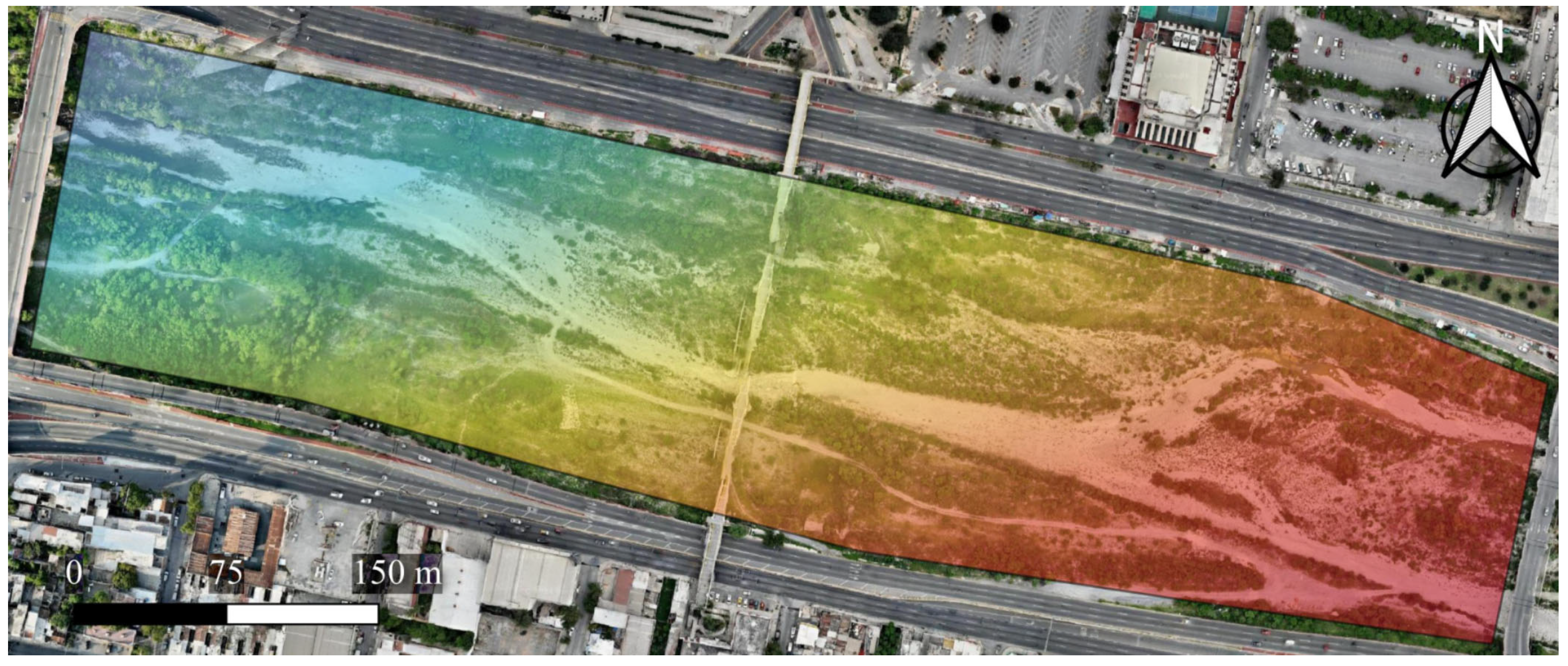
Figure 1. Study area within the Santa Catarina River Basin. Geographic location of the central point of the study area (25°39′50″ N, 100°18′58″ W). The analysis cross-section was delimited using a GIS-based polygon layer derived from a high-resolution georeferenced TIFF image (cropped raster layer).
Hydrology 12 00260 g001
Figure 2. Detailed view of the computational mesh, showing the polyhedral cell structure and refined regions near critical boundaries, such as the riverbed and walls. (a) is the cell size close-up; (b) is the close-up of the inflation layer at the riverbed cells.
Hydrology 12 00260 g002
Figure 3. Contours of instantaneous (or mean) velocity projected onto the iso-surface of volume fraction α = 0.99, representing the evolving free surface of the river. The visualization highlights the three-dimensional flow structure along the channel, with localized regions of high and low velocity resolved by the turbulence models.
Hydrology 12 00260 g003
Figure 4. Comparison of velocity profiles along the central longitudinal line of the computational domain. The graph displays mean velocity values predicted by each turbulence model, allowing for quantitative and qualitative assessment of model performance in reproducing the streamwise flow behavior.
Hydrology 12 00260 g004
Figure 5. Contours of turbulent viscosity μ t mapped onto the iso-surface of volume fraction α = 0.99, representing the river’s free surface. The distribution highlights the spatial variation of momentum diffusivity induced by turbulence across the computational domain.
Hydrology 12 00260 g005
Figure 6. Turbulent viscosity μ t profiles predicted by turbulence models along the central line of the computational domain. The graph illustrates the momentum diffusivity predicted by each turbulence model along the main flow path, highlighting their response to regions of high deformation and localized eddy activity.
Hydrology 12 00260 g006
Figure 7. Contours of strain rate on the iso-surface representing the river’s free surface of volume fraction α = 0.99, comparing predictions from different turbulence models. The visualization highlights spatial variations in flow deformation intensity, with notable differences in maximum strain rate values reflecting each model’s sensitivity to regions of high shear and turbulence anisotropy.
Hydrology 12 00260 g007
Figure 8. Strain rate distribution along the computational domain predicted by various turbulence models. The graph compares the sensitivity of each model to flow deformation gradients, highlighting differences in maximum and minimum values that reflect their treatment of turbulent stress anisotropy and numerical stability.
Hydrology 12 00260 g008
Figure 9. Contours of swirl intensity mapped onto the riverine iso-surface, illustrating the spatial distribution of rotational flow structures predicted by each turbulence model.
Hydrology 12 00260 g009
Figure 10. Swirl intensity along the axial direction, as predicted by each turbulence model. The plot shows the onset and amplification of swirl structures, highlighting differences in model sensitivity to local velocity gradients.
Hydrology 12 00260 g010
Figure 11. Contours of turbulent shear stress ( τ t ) over the iso-surface, highlighting the spatial distribution of momentum transfer due to turbulence across different turbulence models. The figure emphasizes localized regions of elevated stress near channel irregularities and obstacles.
Hydrology 12 00260 g011
Figure 12. Distribution of turbulent shear stress ( τ t ) predicted by each turbulence model along the flow domain. The graph compares the magnitude and variability of τ , revealing differences in sensitivity to local velocity gradients and turbulence intensity.
Hydrology 12 00260 g012
Figure 13. Contours of hydraulic shear stress ( τ h y d r o = ρ u s h 2 ) mapped over the iso-surface of the free surface for the RNG, SST, GEKO, and BSL–EARSM turbulence models. The visualizations depict spatial distribution and relative magnitude.
Hydrology 12 00260 g013
Figure 14. Contours of shear velocity ( u s h ) displayed over the iso-surface of the free surface for the turbulence models RNG, SST, GEKO, and BSL–EARSM. The visualizations illustrate the spatial distribution of near-bed flow intensity, highlighting regions of elevated u s h associated with strong shear and flow-bed interaction, and low u s h zones indicative of recirculation or flow shielding.
Hydrology 12 00260 g014
Figure 15. Iso-surface contours of the Q-criterion showing vortical structures captured by the four turbulence models. SST reaches the highest maximum value, followed by GEKO, BSL–EARSM, and RNG with the lowest. The figure illustrates the spatial distribution and intensity of vortices near the riverbed and throughout the flow domain.
Hydrology 12 00260 g015
Figure 16. Turbulence models’ maximum and minimum Q-criterion values. SST exhibits the highest maximum vortex intensity, followed closely by GEKO and BSL–EARSM, while RNG shows the lowest maximum and the most negative minimum values. This graph highlights the variation in vortex strength and strain among the models.
Hydrology 12 00260 g016
Table 1. Summary and comparative of turbulence model formulations and governing terms.
Models Turbulent   Kinetic   Energy   k Turbulent   Kinetic   Energy   Dissipation   ε
RNG [49] t ρ k + x i ρ k u i = x j α k μ e f f k x j + G k + G b ρ ε Y M + S k t ρ ε + x i ρ ε u i = x j α ε μ e f f ε x j + C 1 ε ε k G k + C 3 ε G b C 2 ε ρ ε 2 k R ε + S ε
SST [51] t ρ k + x i ρ k u i = x j Γ k k x j + G k Y k + S k + G b t ρ ω + x i ρ ω u j = x j Γ ω ω x j + G ω Y ω + S ω + G ω b
GEKO [52] t ρ k + x j ρ k u j = τ i j u i x j C μ ρ k ω + x j μ + μ t σ k k x i t ρ ω + x j ρ ω u = C ω 1 F 1 ω k τ i j u i x j C ω 2 F 2 ρ ω 2 + ρ F 3 C D + x j μ + μ t σ ω ω x i
BLS-EARSM [53,54,55,56] t ρ k + x j ρ u j k = P κ β * ρ ω k + x j μ + σ k μ t k x j t ρ ω + x j ρ u j ω = γ P ω β ρ ω 2 + D ω + x j μ + σ k μ t ω x j
Table 2. Formulations and key terms of turbulence models.
ModelEddy ViscosityTurbulence Production and Source Terms
RNG μ t = ρ C μ k 2 ε , [50,80] G b = β g i μ t P r t T x i
G k = ρ u i u j ¯ u j x i
  G κ = μ t S 2
  S = 2 S i j S i j
SST μ t = ρ k ω [51] G ω = α ω k G k
GEKO μ t = ρ v t = ρ k m a x ω , S C R e a l i z e [52] G b = β g i μ t P r t T x i
  P k = τ i j u i x j
BLS-EARSM μ t = ρ k ω · f μ [53,54,55,56] G b = β g i μ t P r t T x i
  P k = μ t u i x j u i x j + u j x i 2 3 ρ k δ i j u i x j
  P ω = ρ u i x j u i x j + u j x i 2 3 ρ ω δ i j u i x j
Table 3. Velocity metrics across different mesh configurations, including maximum and mean values with relative error estimates based on video-derived observations.
Mesh No.Polyhedral CellsAverage Computing Time u d w m a x
[m/s]
u d w m e a n
[m/s]
u d w m a x
% Error
u d w m e a n
% Error
Overall % Error
1188,9472.5 h10.264.9218.4411.0617.40
2352,0087 h9.544.6610.185.210.16
3591,37912 h8.74.390.460.92.11
4982,61728 h8.64.230.694.510.82
52,500,74347 h8.63.810.6910.995.25
64,228,45890 h8.953.83.5514.473.34
Observation----≈8.66≈4.43------
Table 4. Mean Calculation Times for Various RANS Turbulence Models.
Turbulence ModelMean Calculation Time *
k–ε RNG12.5 h
k–ω SST12 h
k–ω GEKO11.5 h
k–ω BSL–EARSM16 h
* Reported mean calculation times represent typical runtimes observed per model under consistent numerical conditions.
Disclaimer/Publisher’s Note: The statements, opinions and data contained in all publications are solely those of the individual author(s) and contributor(s) and not of MDPI and/or the editor(s). MDPI and/or the editor(s) disclaim responsibility for any injury to people or property resulting from any ideas, methods, instructions or products referred to in the content.