Article

Seasonal Design Floods Estimated by Stationary and Nonstationary Flood Frequency Analysis Methods for Three Gorges Reservoir

1
China Yangtze Power Cooperation Ltd., Wuhan 430010, China
2
State Key Laboratory of Water Resources Engineering and Management, Wuhan University, Wuhan 430072, China
*
Author to whom correspondence should be addressed.
Hydrology 2025, 12(10), 258; https://doi.org/10.3390/hydrology12100258
Submission received: 1 September 2025 / Revised: 28 September 2025 / Accepted: 29 September 2025 / Published: 30 September 2025

Abstract

Highlights

  • The whole flood season of TGR is divided into four sub-periods based on seasonal rainy pattern variation characteristics.
  • Seasonal design floods are estimated using stationary and nonstationary frequency analysis methods.
  • Nonstationary seasonal 1000-year design floods of TGR have reduced by about 20% in the transition period.
  • Flood control water level could rise from 145 m to 157 m, which can generate 2.288 billion kW h more hydropower.

Abstract

Seasonal design floods and operational water levels are critical for high-efficient water resource utilization. In this study, statistical and rational analyses methods were applied to divide the flood season based on seasonal rainfall patterns. The Mann–Kendall test and Theil–Sen analysis were used to detect trend changes in the observed flow series. Both stationary and nonstationary flood frequency analysis methods were conducted to estimate seasonal design floods. The Three Gorges Reservoir (TGR) in the Yangtze River, China, was selected as the case study. Results show that the TGR flood season could be divided into four periods: the reservoir drawdown period (1 May–20 June), the Meiyu flood period (21 June–31 July), the transition period (1 August–10 September), and the Autumn Rain refill period (11 September–31 October). Trend analyses indicate that the flow series at the TGR dam site exhibited a decreasing trend in recent decades. Upstream reservoir regulation has significantly reduced inflow discharges of TGR, and the nonstationary seasonal 1000-year design floods in the transition period are decreased by about 20%, and the flood control water level could rise from 145 m to 157 m, which can generate 2.288 billion kW h more hydropower (16.57% increase) while maintaining unchanged flood prevention standards. This study provides valuable insights into the TGR operational water level in the flood season and highlights the necessity of considering the regulation impact of upstream reservoirs for design floods and reservoir operational water levels.

1. Introduction

Water resources are one of the most important natural resources in the world, holding profound importance for human health, ecosystems, and socioeconomic development [1]. Due to the uneven spatiotemporal distribution of rainfall–runoff in China, the frequent flood disasters and water shortages have significantly constrained economic growth and threatened social stability [2]. To overcome these challenges, numerous reservoirs have been constructed in China for flood control, hydropower generation, water supply, etc., in recent decades [3]. The design floods, defined as floods determined under specified standards, provide critical and theoretical guidance for hydraulic engineering construction and reservoir operation [4].
Traditional flood frequency analysis is the key method for design flood estimation, which relies on the stationary assumption of annual maximum flood data series [5]. However, with climate change and intensified human activities, the hydrological regime has changed significantly. The characteristic values of design floods during the reservoir operation period have deviated considerably from the original design values [6,7], which challenges the stationary assumption and makes the scientifically robust and rational flood frequency analysis under changing conditions more critical for effective reservoir operation and water resource management. In addition, reservoirs play a critical role in flood control, mitigation, and hydropower generation, but in practice, their operation management still relies on the original design floods based on stationarity assumption, without considering the impacts of upstream reservoir regulation on downstream design floods [8]. Therefore, further research is required to investigate the design floods in the reservoir operation period.
Flood limited water level (FLWL) is the critical parameter in reservoir scheduling, as it balances flood control risks and water utilization benefits [9]. The FLWL is determined by the annual maximum design flood and adopted for flood regulation calculations, through which the reservoir can mitigate potential risks from design floods throughout the whole flood season [10]. Nevertheless, under the Asian monsoon climate, flood events exhibit significant seasonal variability, particularly in the Yangtze River basin. Alfieri et al. [11] demonstrated that the most socially disruptive floods predominantly occur in summer in Asia. By investigating the seasonal characteristics of rainfall patterns in the Hanjiang basin, Wang et al. [12] found that the major flood peaks primarily occurred in June–July. Consequently, applying a fixed FLWL throughout the entire flood season is inappropriate, as it results in excessive spill discharges in the flood season and insufficient water storage in the post-flood season [13].
In recent decades, numerous studies have investigated nonstationary flood frequency and its implications for reservoir operation. For instance, Ray and Goel [14] applied the GAMLSS model, integrating climate indices and a reservoir index, to analyze nonstationary flood frequency in the Narmada River basin. They found that the nonstationary models could provide more reliable estimates, and the construction and operation of reservoirs exhibited larger impact on flow discharge than that of climate change. Li et al. [15] developed a nonstationary model to estimate seasonal design floods at the Wulong gauging station in the Wujiang River basin and found that the design floods in August–October were lower than the original design results. They also showed that reservoir regulation flattened seasonal variability under nonstationary conditions. Li et al. [16] applied a nonstationary generalized extreme value (GEV) model to assess the combined effects of upstream reservoir regulation and projected climate change on design flood hydrographs at Yichang hydrological station, demonstrating that future design floods may decrease by 11.4–23.9% compared to the original design values. In addition, related studies on extreme flood risks and resilience have also been widely explored [17,18]. Although previous studies have advanced nonstationary flood frequency analysis and emphasized the role of upstream reservoir regulation, systematic investigations into flood season division and its implications for seasonal design floods and operational water levels remain insufficient, and actionable insights to support reservoir operation are urgently needed.
In this study, the Three Gorges Reservoir (TGR) was selected as a case study, and the stationary and nonstationary flood frequency analysis methods were employed to estimate the seasonal design floods. The specific objectives and novelty are to (a) provide a reasonable flood season division for the TGR; (b) estimate the stationary design flood and corresponding FLWL of TGR based on seasonal maximum natural flow data series; (c) detect the nonstationary characteristics of observed flood data series, and estimate the seasonal design flood and corresponding flood control water level (FCWL) of TGR; and (d) assess and compare the hydropower generation between different operational water levels.
The paper is organized as follows. Section 2 presents the study basin and materials. The methodologies are introduced in Section 3. Section 4 gives seasonal design flood estimation results. Discussions and conclusions are given in Section 5 and Section 6.

2. Study Basin and Materials

2.1. Large-Scale Reservoir Groups in the Upper Yangtze River

The Yangtze River spans approximately 6418 km from its source in the Tanggula Mountains of the Tibetan Plateau to its estuary in the East China Sea. The upper reach is from Geladandong on the Tibetan Plateau to Yichang in Hubei Province, spanning 4511 km and covering a drainage basin area of 1 million km2, and it is characterized by abundant water and hydropower resources. Over recent decades, 117 large-scale reservoirs have been constructed in the upper Yangtze River, which provide 84.2 billion m3 reservoir regulation storage and 50.1 billion m3 flood prevention storage capacity. In this study, a total of 27 key large-scale reservoirs were selected for analysis. Figure 1 illustrates the locations of the key large-scale reservoirs in the upper Yangtze River basin, and the corresponding characteristic parameters of these reservoirs are listed in Table 1.

2.2. Three Gorges Reservoir (TGR)

Located in the mainstream of the Yangtze River basin, Three Gorges Reservoir (TGR) with a basin area of 1 × 10⁶ km2, is the largest hydropower project in China, with a reservoir surface area of about 1080 km2 and an average width of about 1100 m. As one of the largest hydroelectric projects in the world, the TGR plays a key role in the governance of Yangtze River for downstream flood control, hydropower generation, navigation, and water supply. The flood season of the TGR is from June to September during which the flood limited water level (FLWL) is set at 145 m. During the TGR operation period, it employs the FLWL based on the initial design results, maintaining the water level at 145 m during the flood season (from 10 June to 30 September) and then raising it to 175 m (normal storage level) in late October [19].
Since the TGR was put into operation in 2003, the study of FLWL has received a great deal of attention. For example, Liu et al. [20] developed a simulation-optimization model based on copula functions and risk constraints, demonstrating that the dynamic FLWL of TGR can enhance the benefits without increasing flood control risks. A reasonable flood season division can significantly improve TGR hydropower generation and water resource management efficiency. Since a large number of reservoirs have been built in the upper Yangtze River, research on specific quantification of upstream reservoir regulation on seasonal design floods and flood control water levels of TGR is urgently needed [21].
The original design flood of TGR was derived from the stationary flood frequency analysis method based on the annual maximum flood series from 1877 to 1990 at Yichang hydrological station and the investigated historical flood information. By integrating field surveys, literature reviews, gauging station records, archival documents, flood marks, and water level inscriptions, eight major historical flood events in the upper Yangtze River were identified by the Yangtze River Water Resources Commission. Table 2 lists the statistical parameters and original design floods of the Three Gorges Reservoir in the construction period. The 1000-year (0.1% design frequency) design peak discharge (Qm) and 15-day flood volume (W15d) of TGR are 98,800 m3/s and 91.18 billion m3, respectively.

2.3. Data

We used the observed flow data of Yichang hydrological station from 1877 to 2002 and the restored daily flow data of TGR from 2003 to 2022 to form a non-continue annual or seasonal maximum flood data series (from 1877 to 2022), which is regarded as the natural flow data series and used for flood seasonal division and flood frequency analysis.

3. Methodology

In this study, the flow data at the dam site of Three Gorges Reservoir was collected, and the whole flood season was divided into several sub-seasons using statistical and rational analysis methods based on flow data series and seasonal rainfall patterns. Temporal dynamics in each sub-season were analyzed using the Mann–Kendall test and the Theil–Sen estimator. Subsequently, seasonal design floods were estimated using stationary and nonstationary frequency analysis methods. The corresponding design flood hydrographs were derived, and then the stationary FLWL and nonstationary FCWL were determined through reservoir routing calculation. By comparing stationary and nonstationary analysis results of power generation, the impact of upstream reservoir regulation on seasonal design floods and operational water levels were specifically quantified. This study offers valuable insights for water resource management and decision-making in the Yangtze River basin. The research flowchart is shown in Figure 2.

3.1. Flood Seasonal Division Methods

Flood season division methods can be roughly classified into two main types [22]. One is the statistical analysis methods based on observed precipitation or flow data series, which include the relative frequency method [23], directional statistics method [24], probability change point method [25], the entropy-based method [26], etc. The other type is the rational analysis method based on climatic–meteorological seasonal variation characteristics. According to the movement of Asia monsoon winds, rainfall during the flood season in China can be classified into several stages: the main rain belt firstly appears in South China from April to May; the rain belt jumps northward to the middle and lower reaches of the Yangtze River during June and July, which is known as the Meiyu in China [27]; the monsoon rain belt stops in the Yellow and Huaihuai regions to form the Huanghuai rainy season; and then the monsoon rain belt shifts to north and northeast China in July and August. In addition, there is obvious Autumn Rain in southwest China from late August to mid-October [28].

3.2. Detecting Temporal Dynamics of Flow Data Series

To assess whether the stationary assumption is still valid under the changing conditions, the Mann–Kendall (M-K) trend test [29,30] and Theil–Sen (T-S) trend analysis are employed to detect the trend changes in the flow data series. The M-K trend test is a nonparametric statistical approach that assesses the presence and significance of trends in time series, independent of distributional assumptions and undisturbed by outliers, which is calculated using the following equations:
S = i = 1 n 1 j = i + 1 n sgn ( x j x i ) i n , j n
sgn ( x i x j ) = { 1 x j > x i 0 x j = x i 1 x j < x i
V A R ( S ) = 1 18 n ( n 1 ) ( 2 n + 5 ) n 8
Z = { S 1 V A R ( S ) S > 0 0 S > 0 S + 1 V A R ( S ) S < 0
where S denotes the test statistic; x represents the sample series, n is the total number of the sample series; VAR(S) signifies the variance of S; and Z is the standardized test statistic. A value of Z < 0 indicates a decreasing trend in the sample series, whereas a positive Z value (Z > 0) signifies an increasing trend. Additionally, the statistical significance of the trend is determined using the p-value, derived from the standard normal distribution of Z. In this study, a 95% confidence level is adopted, and the trend is statistically significant if p < 0.05.
Likewise, the T-S slope estimator provides robust trend quantification with similar strengths. The T-S trend analysis is
β = m e d i a n ( x j x i j i ) j > i
where β is the trend of variables. The xi and xj are the variable values of the time series at time i and j. If β > 0, it means that the time series is increasing, while if β < 0, it means that the variable is on a decreasing trend.

3.3. Flood Frequency Analysis Method in China

The Pearson type III (P-III) distribution has been recommended by the Ministry of Water Resources as a uniform procedure for flood frequency analysis in China [10]. Let the stationary annual maximum flood data series X follow the P-III distribution with a density function as follows:
f x = β α Γ α x a 0 α 1 e x p β x a 0 a 0 < x < + , 0 < β < + , 0 < α < +
where Γ(·) is the Gamma function; x is a realization of X; and a0, β, and α are the location, scale, and shape parameters of the P-III distribution.
The curve fitting method is recommended by the Ministry of Water Resources in China to estimate parameters of the P-III distribution, where the sum of squared deviations (SSD) criterion is utilized to minimize the discrepancy between the empirical and theoretical frequencies [10]. The P-III distribution coupled with the curve fitting method, denoted as the P3/CF model, has been widely used in China for design flood estimation under the stationary assumption.
When historical flood information is considered, the plotting position formula for non-continuous annual maximum flood data series is expressed as Equation (7). This formula estimates the empirical probability of flood events by integrating both historical floods and observed flood sequences:
F ˜ Y t ( y t ) = P M = M N + 1 M = 1 , 2 , , a P m = 1 N + 1 [ a + N a + 1 n l + 1 ( m l ) ] m = l + 1 , l + 2 , , n
where PM and Pm are the empirical frequency of the Mth extraordinary floods and the mth observed floods, respectively; M represents the flood rank in the extraordinary flood sequence; a is the number of extraordinary floods; N denotes the length of the entire investigation period, which covers the historical information and observed floods; m denotes the flood rank in the observed flood sequence; n is the number of observed floods; and l represents the number of floods identified as extraordinary from the observed floods.
The peak and volume amplitude method are recommended in China for deriving the design flood hydrograph [10]. This method allows the flood peak and volume to be amplified with the same frequency. Let the design flood quantiles estimated by the P3/CF model for a given return period be denoted by flood peak Qm, 1-day maximum flood volume (W1d), 3-day maximum flood volume (W3d), 7-day maximum flood volume (W7d), and 15-day maximum flood volume (W15d), and the design flood hydrograph be derived from the peak and volume amplitude method [31].

3.4. Nonstationary Flood Frequency Analysis Method

When the hydrological data series exhibits nonstationary characteristics, the traditional flood frequency analysis method is inapplicable. The time-varying moment method embeds certain covariates (time variables and physical predictors that have a causal relationship with the hydrological sequence) to explain the variation in the probability distribution parameters for describing the nonstationary characteristics [32].

3.4.1. Time-Varying P-III Distribution

The generalized additive model for location, scale, and shape (GAMLSS) framework could effectively describe the functional relationships between the random variables and covariates [33]. For the three-parameter distribution, the GAMLSS model assumes that μ t , σ t , and ν t represent the time-varying location, scale, and shape parameters of the nonstationary probability distribution f Y t ( y t ) . The yt denotes the sample observation of the response variable Yt (peak discharge or flood volume) at time t. The parameters of μ t , σ t , and ν t are modeled as follows:
g μ μ t = ω 10 + i = 1 I ω 1 i x i t g σ σ t = ω 20 + i = 1 I ω 2 i x i t g ν ν t = ω 30 + i = 1 I ω 3 i x i t
where I denotes the total number of covariates; ω 1 i , ω 2 i , ω 3 i i = 0 , 1 , 2 , , I are the GAMLSS model parameters to be estimated, which can also be represented by Ω ; x i t is the value of the ith covariate at the time t; g μ , g σ , and g ν are the link functions for three time-varying distribution parameters, which could be the identity function, natural logarithm function, or other functions according to the restriction of the sample space.
To consider the regulation impact of the upstream reservoir, the dimensionless Modified Reservoir Index (MRI) derived from reservoir flood prevention storage capacity and the catchment area of the controlled basin is adopted as the covariate in this study [34]. The MRI is calculated by the following equation:
M R I = k = 1 K ( A k A ) ( V k R r )
where K is the total number of the large-scale reservoirs above the study section; k denotes the reservoir number, k = 1, 2, … K; Ak and Vk are the catchment area and the flood prevention storage capacity of the kth reservoir; A and Rr signify the catchment area and the average runoff at the study site. The greater the MRI value, the more significant the impact of upstream reservoir regulation on downstream flood processes.
Extending the conventional P-III distribution within the GAMLSS framework, the time-varying P-Ⅲ distribution considering the MRI is constructed as follows:
f Y t ( y t M R I ; Ω ) = β t α t Γ ( α t ) ( y t a 0 t ) α t 1 e β t ( y t a 0 t )
where yt is the observed flood data series at time t; f Y t ( y t M R I ; Ω ) is the probability density function of the time-varying P-III distribution corresponding to yt; Ω = ω 1 i , ω 2 i , ω 3 i i = 0 , 1 , 2 , , I is the set of GAMLSS model parameters; I is the total number of covariates, in this study, I = 1; Γ ( ) is the Gamma function; and a 0 t , α t , and β t are the location, shape, and scale parameters of time-varying P-III distribution, respectively, where β t > 0 , α t > 0 .

3.4.2. Time-Varying P-III Distribution Curve Fitting Method

Like the stationary P-III distribution curve fitting method (denoted as the P3/CF model), the time-varying P-III distribution curve fitting method proposed by Xie et al. [35], denoted as the Tv-P3/CF model, is used for nonstationary flood frequency analysis in China. The Q-Q (Quantile–Quantile) plot, with the inverse cumulative distribution function of the Gamma distribution as the coordinate axis, is also employed. The method of the Q–Q plot is used to fit the empirical and the theoretical frequencies as follows:
G 1 z ˜ t | α , β , G 1 z t | α , β ; t = 1 , 2 , , n + a l
where G 1 z t | α , β is the inverse cumulative distribution function of the Gamma distribution when the distribution function value equals zt; α and β are the shape and scale parameters of the Gamma distribution, respectively. To ensure that the Gamma distribution retains its bell-shaped and right-skewed density curve, which emphasizes the fitting of extraordinary floods, α and β are set to be consistent with those of the P-III distribution frequency curve from the initial design flood values, which ensures that the theoretical distribution could capture the characteristics of flood events.

4. Seasonal Design Flood Estimation Results

4.1. Flood Seasonal Division for TGR

Extreme floods tend to occur predominantly during a specific period in the rainstorm season; however, the conventional flood limited water level (FLWL) is determined by annual maximum flood data series, which ignores hydrologic seasonal variations [36]. Based on the distinct seasonality of regional flood patterns, the whole flood season is typically divided into several sub-periods [37]. In the main flood period, characterized by high flood risk, reservoir operations must maintain water levels below the FLWL to ensure flood control safety. In other periods with lower flood risk, a higher reservoir operation water level is allowed to enhance storage and hydropower generation. Studies confirmed that the application of seasonally adjusted water level is suitable for the Yangtze River basin, where flood seasonality is well-defined and reservoir operations typically follow a drawdown–refill cycle [38].
Based on natural flood data series and statistical analysis methods, the whole flood season of TGR has been divided into pre-flood season (from 1 May to 20 June), main-flood period (from 21 June to 10 September), and post-flood period (from 11 September to 30 October) [20]. Since the Meiyu and Autumn Rain are two major seasonal rainy patterns in the Yangtze River basin, they exhibit distinct temporal variation characteristics. The Meiyu typically begins in June and ends in late July, while the Autumn Rain in western China generally starts in early September and lasts until late October [12]. Based on these hydrometeorological patterns and reservoir operation cycle, the TGR whole flood season could be further divided into four periods, i.e., the drawdown period (from 1 May to 20 June), the Meiyu flood period (from 21 June to 31 July), the transition period (from 1 August to 10 September), and the Autumn Rain refill period (from 11 September to 30 October).
During the Meiyu flood period (from 21 June to 31 July), when flood control risk is highest due to the Meiyu occurring in the middle reach of the Yangtze River, TGR operates under the FLWL derived from the annual maximum flood series to ensure flood control safety. After the end of Meiyu, the reserved flood prevention storage capacity of TGR could be released gradually and raise the operational water level in the transition period from 1 August to 10 September. As Autumn Rain starts, most upstream reservoirs begin to refill and substantially reduce the inflow discharge of TGR, and the operation water level could be further raised to the normal water level from 11 September to 30 October. This study mainly focuses on estimating seasonal design floods and corresponding seasonal water levels in the transition period, both using stationary and nonstationary flood frequency analysis methods.

4.2. Stationary Seasonal Flood Frequency Analysis Results

The data incorporates both restored natural flow data from 1877 to 2022 and three investigated historical floods that occurred in 1153, 1227, and 1560 in the transition period from 1 August to 10 September, as shown in Table 3. The P3/CF model, recommended by the Ministry of Water Resources of China, is used to estimate seasonal design floods [10]. Table 4 lists the seasonal design floods of TGR estimated by the P3/CF model in the transition period from 1 August to 10 September. Compared with Table 2, the estimated seasonal design floods during the transition period are less than those of the original design floods estimated from the annual maximum flood data series. For example, the 1000-year design 15-day flood volume W15d is reduced by 7.63%.
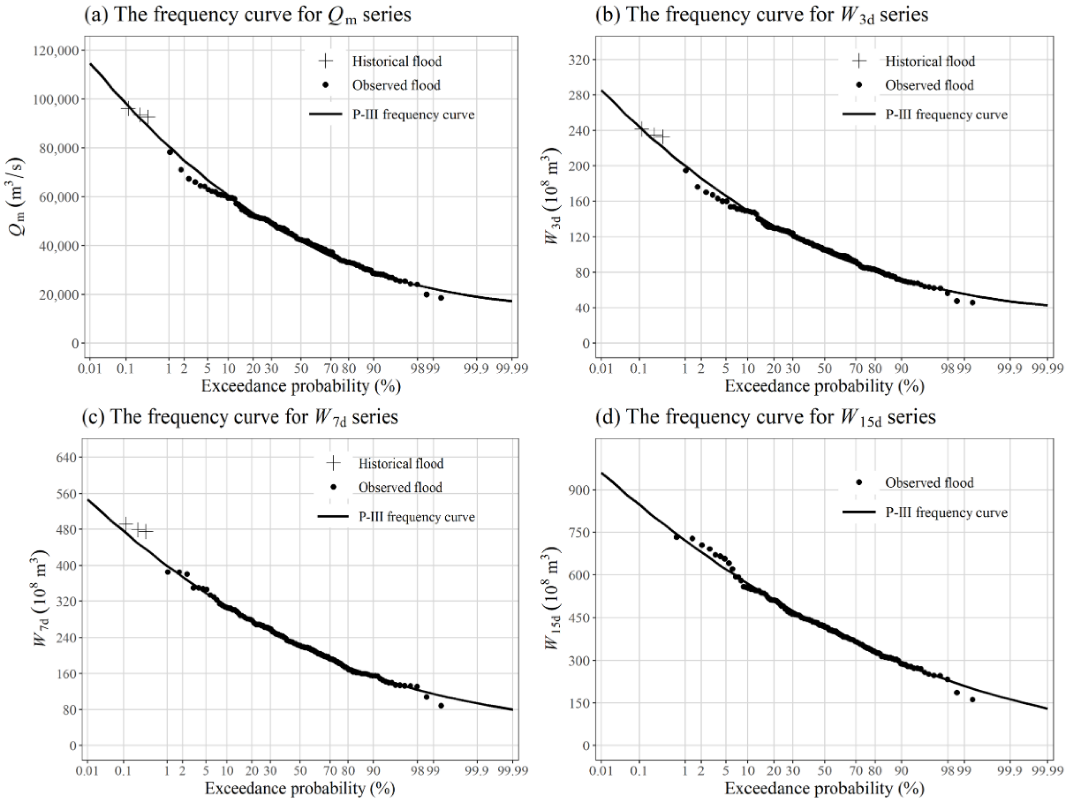
Figure 3 plots the seasonal P-III frequency curves of TGR in the transition period from 1 August to 10 September, where the plotting position formula (Equation (7)) is used to calculate the empirical frequencies. It is shown that P-III frequency curves can fit flood data points very well.

4.3. Nonstationary Flood Frequency Analysis Results

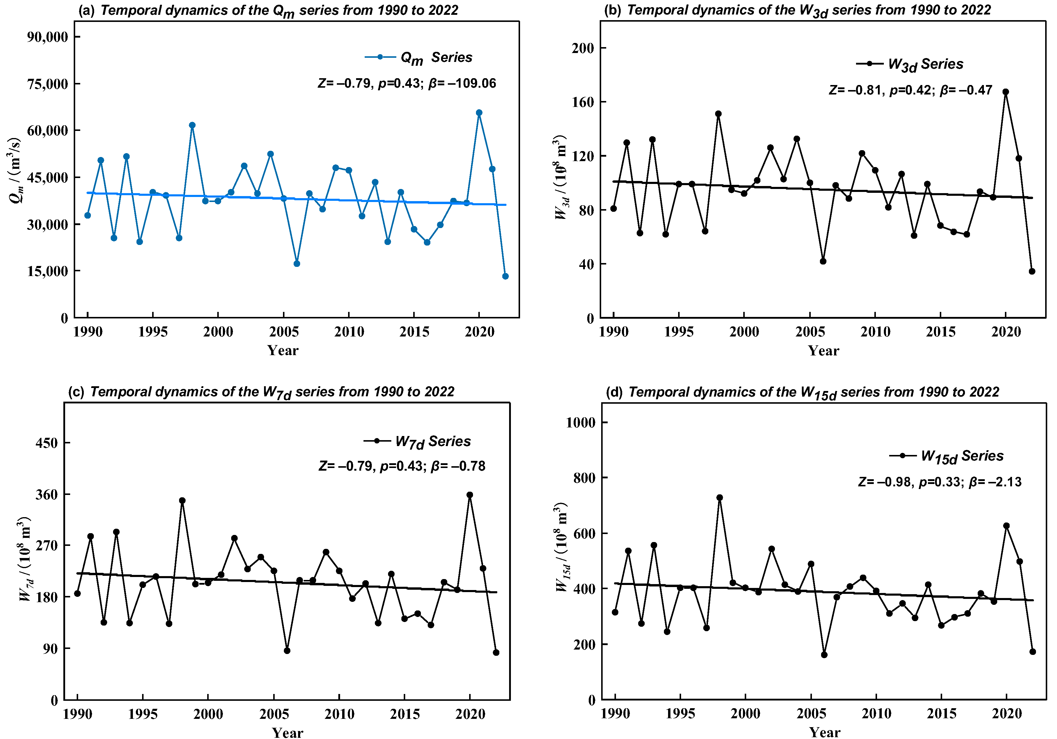
Since most reservoirs were built after 1990 in the upper Yangtze River basin, the Mann–Kendall (M-K) trend test and Theil–Sen (T-S) trend analysis are used to detect the change trend using the observed flood data in the transition period from 1990 to 2022. Figure 4 shows the temporal dynamics of the seasonal maximum flood data series in the transition period from 1990 to 2022. It can be seen that the observed flood data series exhibits a consistent decreasing trend in the transition period, which confirms that the assumption of stationarity no longer exists. Hence, the traditional flood frequency analysis methods are inappropriate for such nonstationary flow data series.
Figure 5 depicts the variation trends of the MRI at the TGR dam site for the transition period. It is evident that with the construction and operation of key large-scale reservoirs in the upper Yangtze River since the late 1990s, the MRI has exhibited a stepwise increasing trend. According to the reservoir operation year (Table 1), there were seven large-scale reservoirs put into operation in 2014, which predominantly influence the MRI, followed by those commissioned in 2021–2022. The regulation of these reservoirs has significantly altered the downstream hydrological regime and reduced the inflow discharges of TGR.
Regarding the determination of link functions, since the location parameter a 0 t of the time-varying P-III distribution would become negative when Cv/Cs ≤ 2, the identity functions are adopted to facilitate the parameter estimation using the following equations:
a 0 t = ω 10 + ω 11 × M R I β t 1 = ω 20 + ω 21 × M R I α t = ω 30
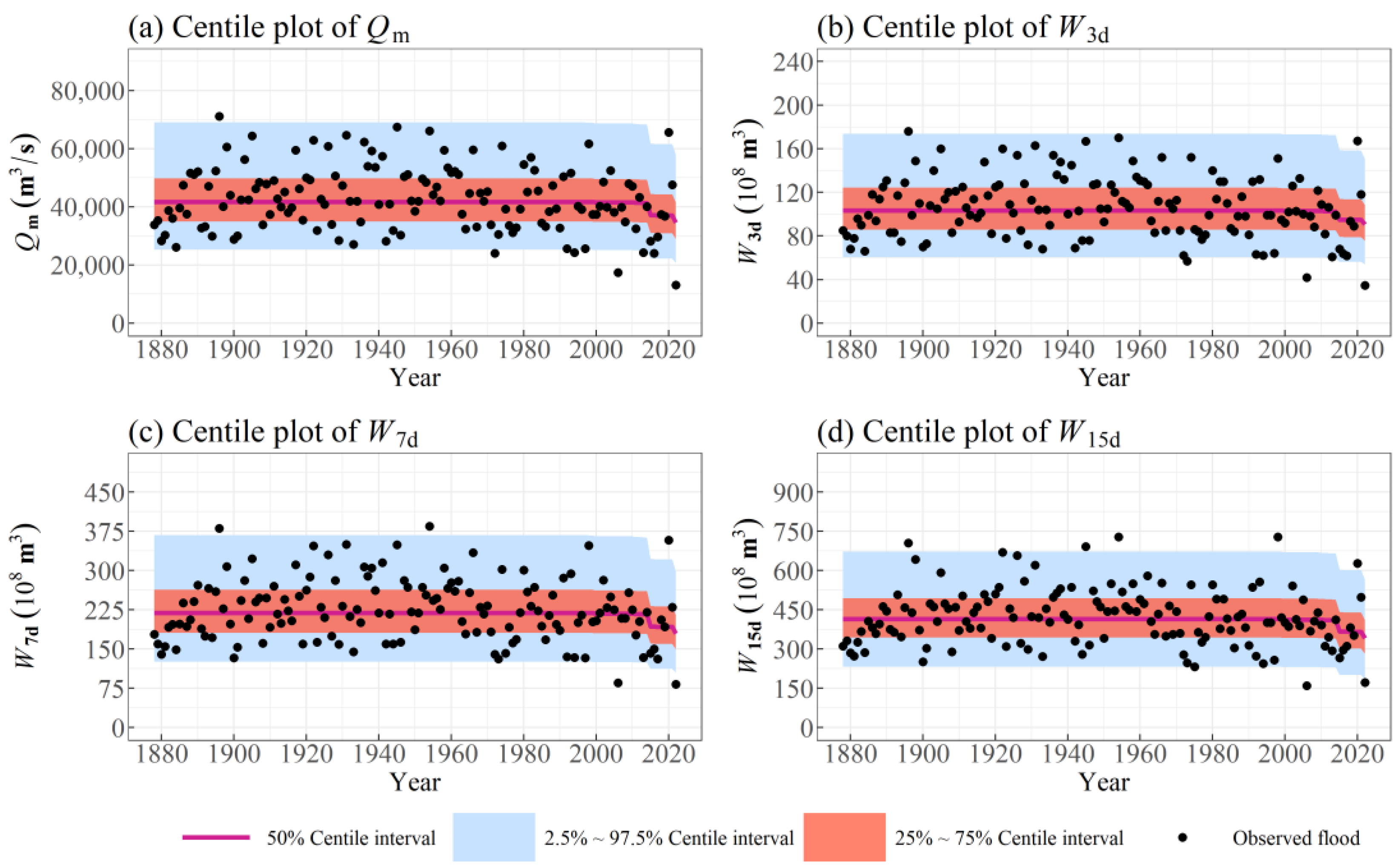
The minimum sum of squared differences (SSD) criterion, as recommended by the Ministry of Water Resources of China, is employed to fit the empirical frequencies to theoretical frequencies of the time-varying P-III distribution. In addition, the Kolmogorov–Smirnov (K-S) test, Akaike Information Criterion (AIC) [39], and centile curve plots are utilized to diagnose and evaluate the fitting results. The K-S test detects whether the cumulative distribution function of the theoretical distribution conforms to a standard uniform distribution on (0, 1). Setting the significance level of 0.05, a p-value > 0.05 in the K-S test indicates the model passes the test, confirming the validity of the time-varying P-III model. The AIC is employed to assess the goodness of fit, where the smaller AIC value indicates the better model fit. Centile curve plots can evaluate the model’s performance by examining the distribution of sample data across different centile intervals, where greater uniformity reflects the better fit.
Table 5 presents the estimated parameters and test results in the transition period from 1 August to 10 September, in which the p-values of the K-S test all exceed 0.05, confirming the suitability of the time-varying P-III model. The negative estimates of parameters ω 11 and ω 21 further validate that the MRI can effectively reflect the regulation impact of upstream reservoirs.
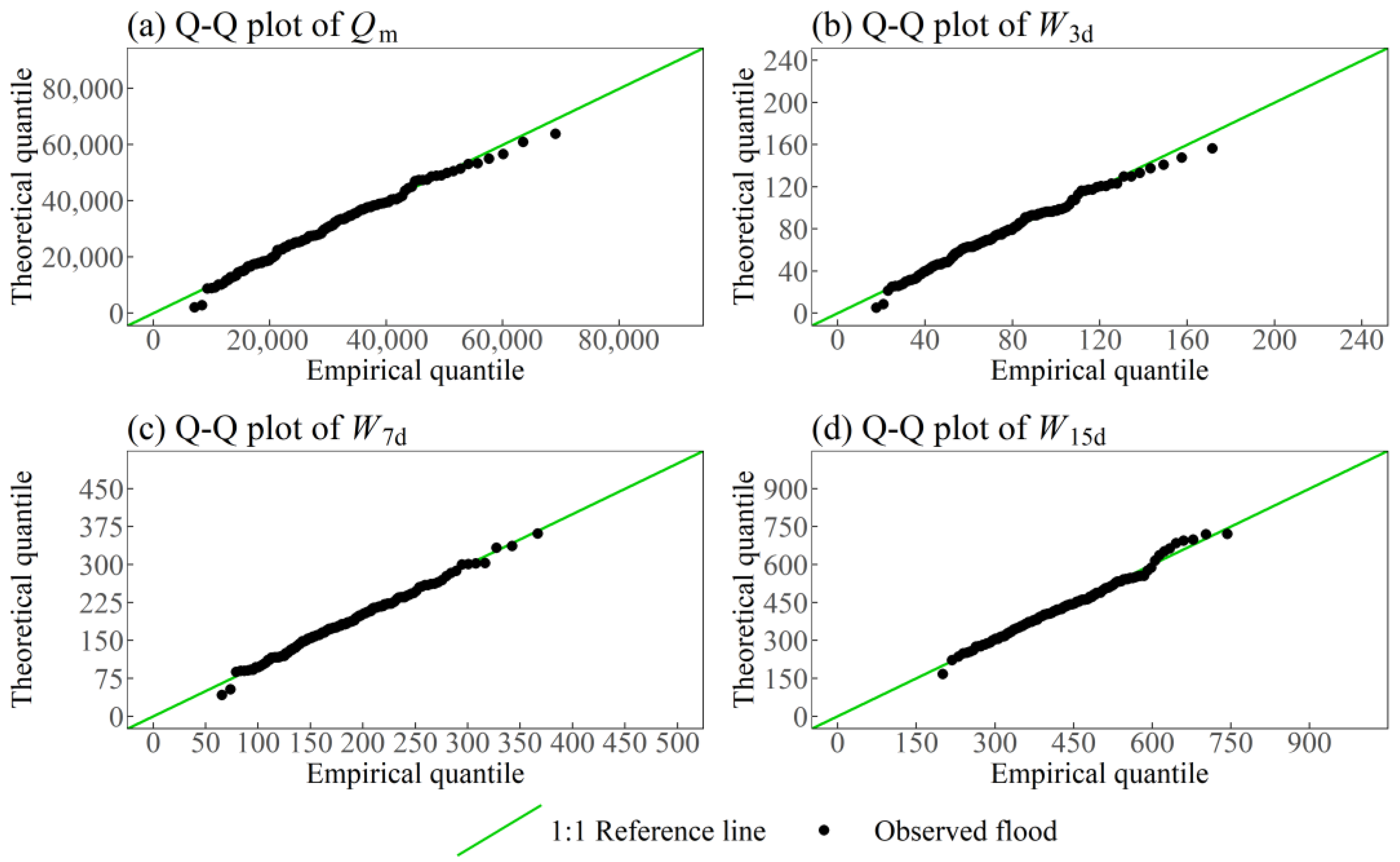
Figure 6 and Figure 7 show the Q-Q plot and the centile plot for the flood data series in the TGR transition period from 1 August to 10 September. They provide further evidence of the robust model fit to the flood data series in the transition period, as demonstrated by the centile and Q-Q plots.
This study focuses on estimating nonstationary design floods for given 20-, 100-, and 1000-year return periods. Table 6 compares the nonstationary seasonal design floods estimated by the Tv-P-III/CF model in the TGR transition period from 1 August to 10 September. For the statistical parameters, the mean of the flood series derived from the nonstationary flood frequency analysis is significantly lower than the stationary flood frequency results, and Cv and Cs exhibit little change. Affected by upstream reservoir regulation, the estimates at specific design frequencies show a notable reduction in design floods. Taking the 1000-year design floods as an example, the peak discharge (Qm) and W15d flood volume have reduced by 22.9% and 14.3%, respectively.
Figure 8 further illustrates these differences by comparing the stationary and nonstationary P-III flood frequency curves in the transition period, which shows that while the stationary P-III curve aligns well with the empirical frequency points, while the nonstationary P-III curve consistently lies below it.

4.4. Derive Seasonal Design Flood Hydrograph and Flood Limited/Control Water Level

The design flood hydrograph was derived using the typical flood hydrograph method combined with the peak–volume amplitude scaling algorithm, which has been recommended by the Ministry of Water Resources of China [10]. The flood event with the highest peak discharge or largest flood volume is often selected as the typical flood hydrograph. In this study, a severe flood event that occurred in the upper Yangtze River basin in 1981 was selected as the typical flood hydrograph. Based on the seasonal design flood estimates, the selected typical flood hydrograph is then amplified using the same frequency amplification method to obtain the seasonal design flood hydrograph [31].
Figure 9 compares the 1000-year seasonal design flood hydrographs derived from stationary and nonstationary methods in the transition period from 1 August to 10 September. It is evident that upstream reservoir regulation substantially reduces the inflow flood magnitudes of the TGR. The nonstationary design hydrographs lie below the stationary design hydrograph, exhibiting a more flattened flood process, which confirms the substantial reduction in downstream design floods due to the regulation of upstream cascade reservoirs.
According to the TGR operation rules, the characteristic reservoir water levels were derived from the flood routing iterative simulations while ensuring the flood control standards remained unchanged. Based on the 1000-year seasonal design flood hydrographs, the stationary FLWL and nonstationary FCWL of the TGR in the transition period were determined using the reservoir flood routing calculation method. The results, along with current FLWL values, are presented in Table 7. Compared with the original FLWL of 145 m based on the stationary annual maximum flood data series, the seasonal FLWL of TGR could be raised to 149 m, while the nonstationary seasonal FCWL can be further raised to 157 m in the transition period from 1 August to 10 September.

4.5. Hydropower Benefit Analysis

A hydropower benefit analysis model is proposed to compare the impact of different operation water levels on hydropower generation, which is given as follows:
E ¯ = i = 1 M t = 1 T N i ( t ) Δ t / M N i ( t ) = K Q i ( t ) H i ( t )
where E ¯ denotes the multi-year average hydropower generation during the flood season, kW·h; N i ( t ) is the hydropower output of the ith year in period t, MW; Δ t is the time step, day; M presents the number of years; T is the total time steps during the flood season per year; K represents hydropower efficiency of the ith reservoir, constant; Q i ( t ) denotes flow discharge release from turbines of the ith reservoir in period t, m3/s; and H i ( t ) is the average hydropower head of the ith reservoir in period t, m. Additionally, the reservoir operation model is subject to multiple constraints, including water balance, reservoir water level limits, outflow restrictions, water level fluctuation rate, and boundary conditions.
Based on the TGR operation rules and the daily flow data from 2003 to 2022, the hydropower benefits were evaluated with different FLWL/FCWL, while keeping the flood control standards unchanged. It should be noted that these estimates are based on simplified assumptions of constant turbine efficiency and idealized operation of all units. Table 7 compares the hydropower generation with different design schemes in the transition period from 1 August to 10 September. Compared with the current annual FLWL schemes, the hydropower generation under the stationary seasonal FLWL scheme could increase about 0.955 billion kW·h (or increase 6.92%). The nonstationary seasonal FCWL scheme considered the regulation effect of upstream reservoirs can further increase hydropower generation by 2.288 billion kW·h (or increase 16.57%). These results underscore the importance of flood season division for the TGR and highlight the critical role of upstream reservoir regulation in enhancing the TGR’s comprehensive benefits.

5. Discussion

A large number of reservoirs have been constructed and operated in the upper Yangtze River basin, substantially altering the inflow flood processes of the TGR. The stationary assumption of flood data series is fundamental for the conventional flood frequency analysis, which has been increasingly challenged under the impact of climate change and intensified human activities. Numerous studies have shown that the regulation effects of cascade reservoirs are greater than those of climate change [1,7,14,15,16]. Once the hydrological series exhibits nonstationary behavior, which means the stationary assumption no longer exists, the traditional flood frequency analysis method is inapplicable. Therefore, the nonstationary flood frequency analysis methods have been developed to estimate design floods. Among them, the time-varying moment framework introduces covariates into the distribution parameters to capture nonstationary characteristics. The maximum likelihood method [40] and the least squares method [41] are the most widely adopted techniques for parameter estimation. Recently, Xie et al. [35] proposed the time-varying P-III distribution curve-fitting (Tv-P-III/CF) method, which has been increasingly applied in China for nonstationary flood frequency analysis.
Prior to applying stationary or nonstationary models, it is crucial to perform robust trend diagnostics to ensure the validity and applicability of the stationary or nonstationary flood frequency analysis. The Mann–Kendall (M–K) and Theil–Sen (T–S) tests reveal a consistent decreasing trend in the TGR flood series (Figure 4). Similarly, Hu et al. [21] identified nonstationary tendencies in flood data series at the Cuntan and Yichang stations in the Yangtze River, further confirming that the stationarity assumption no longer holds in this region. In this case, the Tv-P-III/CF model provided an effective framework for seasonal design flood estimation by incorporating the covariate MRI to explicitly capture the regulatory impacts of upstream reservoirs. This model was employed to estimate the nonstationary seasonal design floods of the TGR. In addition, flood routing simulations were conducted to assess the influence of upstream reservoir regulation on seasonal FCWL, while flood benefit analyses were used to quantify its benefits for hydropower generation. By integrating these methodological components, we not only provide a refined assessment of reservoir operation under nonstationary conditions, quantifying the impact of the upstream reservoir regulation, but also address a critical knowledge gap in the theoretical understanding of seasonal operational rules for the TGR, thereby offering insights of both scientific and practical significance.
Table 5 presents the parameter estimations of the Tv-P3/CF model in the transition period. The parameters ω 11 and ω 21 are both negative, confirming the reduction in inflow due to the regulation effect of upstream reservoir. Compared to the previous study, the parameters ω 10 , ω 20 , and ω 30 exhibit differences across the seasonal maximum flood data series; this is because the curve fitting statistics for the sub-period exist in the relationship of Cs/Cv ≤ 2, leading to the unavailable estimation of parameter a 0 t in the P-Ⅲ distribution [10]. Additionally, affected by the larger mean values and variance of the seasonal maximum flood data series, the SSD of the W7d and W15d display higher values than the W3d. The estimated design floods in the transition period are presented in Table 6, indicating that upstream reservoir regulation has reduced the design floods in the TGR operation period by approximately 10–20% compared to the stationary seasonal analysis results. Previous studies reported that the 1000-year design floods for the Xiangjiaba Reservoir were reduced by approximately 40% [42], where there are 13 large reservoirs constructed in the Jinsha River basin, as shown in Figure 1 and Table 1. However, the available reservoir storage in the Minjiang, Jialing, and Wujiang River basins is relatively small, while the controlled drainage area of TGR is nearly twice that of Xiangjiaba Reservoir. Therefore, the flood peak reduction rate of TGR should be lower than that of Xiangjiaba Reservoir. The results obtained in this study are consistent with these findings, further confirming the robustness and reliability of the study.
Although our investigation reported here systematically evaluates the regulation impact of upstream reservoirs on the seasonal design floods and corresponding FCWL of TGR, there are still some unavoidable uncertainties and limitations. First, inevitable uncertainties arise from the flood data series. As the sensitive input variables of the flood frequency analysis, the annual or seasonal maximum sampling methods will affect the final analysis results. To closely align with the original flow data series, this study utilized flow data (1877–2002) at the Yichang hydrologic station and converted TGR inflow data (2003–2022); however, the biases are still unavoidable. In addition, although this study applied only the Tv-P-III/CF method, whose reliability has been validated through comparison with other approaches [35], the alternative methods, such as the flood regional composition method [42], were not adopted. In addition, due to the primary focus on quantifying regulatory effects on seasonal design floods and operational water levels, confidence intervals for design flood and hydropower estimates were not calculated. Moreover, the increase in hydropower is based on the simplified assumptions of constant turbine efficiency and idealized unit operation, without accounting for detailed variations between peaking and base load operations. A more comprehensive analysis of seasonal design floods and operational water levels in the reservoir operation period will be conducted in future research.

6. Conclusions

The stationary and nonstationary flood frequency analysis methods were applied to estimate seasonal design floods, and corresponding seasonal operation water levels were determined for the Three Gorges Reservoir. The main conclusions are summarized as follows:
(1)
The whole flood season of TGR can be divided into four periods, i.e., the reservoir drawdown period (1 May to 20 June), the Meiyu flood period (21 June to 31 July), the transition period (1 August to 10 September), and the Autumn Rain refill period (11 September to 30 October).
(2)
The time-varying P-III curve fitting method was employed to estimate the seasonal design floods in the transition period. Compared to the original design values, 1000-year seasonal design peak discharge and 15-day flood volume are reduced by 22.9% and 14.3%, respectively.
(3)
Nonstationary seasonal FCWL could be raised up from 145 m to 157 m while maintaining unchanged flood control standards, which can generate 2.288 billion kW·h more hydropower (or increase 16.57%) in the transition period from 1 August to 10 September.
Overall, this study provides valuable insights into quantifying the regulation impact of upstream reservoirs on the TGR seasonal design floods, offering theoretical support for real-time reservoir operation for increasing hydropower generation, and also contributes to the objectives of SDG 6 (Clean Water and Sanitation) and SDG 7 (Affordable and Clean Energy), and thus supports wider socioeconomic well-being.

Author Contributions

B.S.: writing—original draft writing, visualization, methodology, formal analysis, data curation. S.G.: conceptualization, review and editing, project administration, funding acquisition. S.Z.: conceptualization, data curation. X.W.: data curation, calculation. N.L.: data curation, calculation. All authors have read and agreed to the published version of the manuscript.

Funding

This research was funded by the China Yangtze Power Cooperation Ltd. (Z242402005) and National Natural Science Foundation of China (No. U2340205).

Data Availability Statement

Some or all data and models that support the findings of this study are available from the corresponding author upon reasonable request.

Acknowledgments

The authors would like to thank the editor and anonymous reviewers whose comments and suggestions have helped to improve the manuscript.

Conflicts of Interest

Authors Bokai Sun and Na Li were employed by company China Yangtze Power Cooperation Ltd. The remaining authors declare that the research was conducted in the absence of any commercial or financial relationships that could be construed as a potential conflict of interest.

References

  1. Jain, S.K.; Shilpa, L.S.; Rani, D.; Sudheer, K.P. State-of-the-art review: Operation of multi-purpose reservoirs during flood season. J. Hydrol. 2023, 618, 129165. [Google Scholar] [CrossRef]
  2. Mohammadi, P.; Ebrahimi, K.; Bazrafshan, J. Flood frequency analysis under nonstationary modeling in the Gorganrood River basin, Iran. J. Hydrol. Eng. 2023, 28, 05023004. [Google Scholar] [CrossRef]
  3. Wang, Z.; Wang, Y.; Liu, K.; Cheng, L.; Cai, X. Theory and practice of basin-wide floodwater utilization: Typical implementing measures in China. J. Hydrol. 2024, 628, 130520. [Google Scholar] [CrossRef]
  4. He, S.; Li, B.; Li, Q.; Zheng, H.; Chen, Y. Refining hydropower operation by dynamic control of cascade reservoir water levels with flood season segmentation. Energy 2025, 314, 134156. [Google Scholar] [CrossRef]
  5. Cunnane, C. Statistical Distribution for Flood Frequency Analysis; Operational Hydrology Report, WMO, No.718; WMO: Geneva, Switzerland, 1989. [Google Scholar]
  6. Huang, K.; Ye, L.; Chen, L.; Wang, Q.; Dai, L.; Zhou, J.; Singh, V.P.; Huang, M.; Zhang, J. Risk analysis of flood control reservoir operation considering multiple uncertainties. J. Hydrol. 2018, 565, 672–684. [Google Scholar] [CrossRef]
  7. Milly, P.C.; Betancourt, J.; Falkenmark, M.; Hirsch, R.M.; Kundzewicz, Z.W.; Lettenmaier, D.P.; Stouffer, R.J. Stationarity is dead: Whither water management? Science 2008, 319, 573–574. [Google Scholar] [CrossRef]
  8. Zhao, G.; Bates, P.; Neal, J. The impact of dams on design floods in the conterminous US. Water Resour. Res. 2020, 56, e2019WR025380. [Google Scholar] [CrossRef]
  9. Ouyang, S.; Zhou, J.; Li, C.; Liao, X.; Wang, H. Optimal design for flood limit water level of cascade reservoirs. Water Resour. Manag. 2015, 29, 445–457. [Google Scholar] [CrossRef]
  10. MWR (Ministry of Water Resources of China). Specification for Calculating Design Flood of Water Resources and Hydropower Projects; China Water & Power Press: Beijing, China, 2006. (In Chinese) [Google Scholar]
  11. Alfieri, L.; Dottori, F.; Salamon, P.; Wu, H.; Feyen, L. Global modeling of seasonal mortality rates from river floods. Earth Future 2020, 8, e2020EF001541. [Google Scholar] [CrossRef]
  12. Wang, X.; Guo, S.; Zhong, S.; Wang, M.; Xiang, X. Flood season division using statistical analysis methods and verifying by regional rainy characteristics. Water 2024, 16, 3677. [Google Scholar] [CrossRef]
  13. Jiang, M.; Qiao, C.; Lu, F.; Zhu, K.; Zhu, C. The impact of reservoirs with seasonal flood limit water level on the frequency of downstream floods. J. Hydrol. 2024, 644, 132009. [Google Scholar] [CrossRef]
  14. Ray, L.K.; Goel, N.K. Flood frequency analysis of Narmada River basin in India under nonstationary condition. J. Hydrol. Eng. 2019, 24, 05019018. [Google Scholar] [CrossRef]
  15. Li, W.; Xiong, L.; Zhou, Y.; Yin, J.; Li, R.; Chen, J.; Liu, D. Nonstationary seasonal design flood estimation: Exploring mixed copulas for the nonmonotonic dependence between peak discharge and timing. J. Hydrol. Eng. 2024, 29, 04023046. [Google Scholar] [CrossRef]
  16. Li, R.; Xiong, L.; Zha, X.; Xiong, B.; Liu, H.; Chen, J.; Zeng, L.; Li, W. Impacts of climate and reservoirs on the downstream design flood hydrograph: A case study of Yichang Station. Nat. Hazards 2022, 113, 1803–1831. [Google Scholar] [CrossRef]
  17. Falter, D.; Dung, N.V.; Vorogushyn, S.; Schröter, K.; Hundecha, Y.; Kreibich, H.; Apel, F.; Merz, B. Continuous, large-scale simulation model for flood risk assessments: Proof-of-concept. J. Flood Risk Manag. 2016, 9, 3–21. [Google Scholar] [CrossRef]
  18. Nazari, R.; Vasiliadis, H.; Karimi, M.; Fahad, M.G.R.; Simon, S.; Zhang, T.; Sun, Q.; Peters, R. Hydrodynamic study of the impact of extreme Flooding events on wastewater treatment plants considering total water level. Nat. Hazards Rev. 2022, 23, 04021056. [Google Scholar] [CrossRef]
  19. Xu, Z.; Mo, L.; Zhou, J.; Zhang, X. Optimal dispatching rules of hydropower reservoir in flood season considering flood resources utilization: A case study of Three Gorges Reservoir in China. J. Clean. Prod. 2023, 388, 135975. [Google Scholar] [CrossRef]
  20. Liu, P.; Li, L.; Guo, S.; Xiong, L.; Zhang, W.; Zhang, J.; Xu, C.Y. Optimal design of seasonal flood limited water levels and its application for the Three Gorges Reservoir. J. Hydrol. 2015, 527, 1045–1053. [Google Scholar] [CrossRef]
  21. Hu, Y.; Cao, Z.; Chen, Y.; Hu, J.; Guo, J.; Liang, Z. Nonstationary multi-site design flood estimation and application to design flood regional composition analysis. J. Hydrol. 2024, 638, 131538. [Google Scholar] [CrossRef]
  22. Black, A.R.; Werritty, A. Seasonality of flooding: A case study of North Britain. J. Hydrol. 1997, 195, 1–25. [Google Scholar] [CrossRef]
  23. Cunderlik, J.M.; Ouarda, T.B.M.J.; Bobée, B. Determination of flood seasonality from hydrological records. Hydrol. Sci. J. 2004, 49, 11. [Google Scholar] [CrossRef]
  24. Chen, L.; Singh, V.P.; Guo, S.; Fang, B.; Liu, P. A new method for identification of flood seasons using directional statistics. Hydrol. Sci. J. 2013, 58, 28–40. [Google Scholar] [CrossRef]
  25. Liu, P.; Guo, S.; Xiong, L.; Chen, L. Flood season segmentation based on the probability change-point analysis technique. Hydrol. Sci. J. 2010, 55, 540–554. [Google Scholar] [CrossRef]
  26. Xiong, F.; Guo, S.; Chen, L.; Chang, F.J.; Zhong, Y.; Liu, P. Identification of flood seasonality using an entropy-based method. Stoch. Environ. Res. Risk Assess. 2018, 32, 3021–3035. [Google Scholar] [CrossRef]
  27. Xu, X.; Lu, C.; Shi, X.; Ding, Y. Large-scale topography of China: A factor for the seasonal progression of the Meiyu rainband? J. Geophys. Res. Atmos. 2010, 115, 2009JD012444. [Google Scholar] [CrossRef]
  28. Zhang, C.; Wang, Z.; Zhou, B.; Li, Y.; Tang, H.; Xiang, B. Trends in autumn rain of West China from 1961 to 2014. Theor. Appl. Climatol. 2019, 135, 533–544. [Google Scholar] [CrossRef]
  29. Mann, H. Nonparametric tests against trend. Econometrica 1945, 13, 245–259. [Google Scholar] [CrossRef]
  30. Kendall, M.; Gibbons, J. Rank Correlation Methods, 5th ed.; Griffin: London, UK, 1990. [Google Scholar]
  31. Xiao, Y.; Guo, S.; Liu, P.; Yan, B.; Chen, L. Design flood hydrograph based on multicharacteristic synthesis index method. J. Hydrol. Eng. 2009, 14, 1359–1364. [Google Scholar] [CrossRef]
  32. Strupczewski, W.G.; Singh, V.P.; Mitosek, H.T. Nonstationary approach to at-site flood frequency modelling. III. Flood analysis of Polish Rivers. J. Hydrol. 2001, 248, 152–167. [Google Scholar] [CrossRef]
  33. Rigby, R.; Stasinopoulos, D. Generalized additive models for location, scale and shape. J. R. Stat. Soc. Ser. C Appl. Stat. 2005, 54, 507–554. [Google Scholar] [CrossRef]
  34. Cui, H.; Jiang, S.; Gao, B.; Ren, L.; Xiao, W.; Wang, M.; Ren, M.; Xu, C.Y. On method of regional non-stationary flood frequency analysis under the influence of large reservoir group and climate change. J. Hydrol. 2023, 618, 129255. [Google Scholar] [CrossRef]
  35. Xie, Y.; Guo, S.; Zhong, S.; Wang, X.; Tian, J.; Liang, Z. A novel time-varying P-III distribution curve fitting model to estimate design floods in Three Gorges Reservoir operation period. Hydrology 2024, 11, 203. [Google Scholar] [CrossRef]
  36. Gao, S.; Liu, P.; Pan, Z.; Ming, B.; Guo, S.; Cheng, L.; Wang, J. Incorporating reservoir impacts into flood frequency distribution functions. J. Hydrol. 2019, 568, 234–246. [Google Scholar] [CrossRef]
  37. Zhou, Y.; Guo, S. Risk analysis for flood control operation of seasonal flood-limited water level incorporating inflow forecasting error. Hydrol. Sci. J. 2014, 59, 1006–1019. [Google Scholar] [CrossRef]
  38. Xiong, B.; Xiong, L.; Guo, S.; Xu, C.Y.; Xia, J.; Zhong, Y.; Yang, H. Nonstationary frequency analysis of censored data: A case study of the floods in the Yangtze River from 1470 to 2017. Water Resour. Res. 2020, 56, e2020WR027112. [Google Scholar] [CrossRef]
  39. Akaike, H. A new look at the statistical model identification. IEEE Trans. Autom. Control 1974, 19, 716–723. [Google Scholar] [CrossRef]
  40. Strupczewski, W.G.; Singh, V.P.; Feluch, W. Nonstationary approach to at-site flood frequency modelling I. Maximum likelihood estimation. J. Hydrol. 2001, 248, 123–142. [Google Scholar] [CrossRef]
  41. Strupczewski, W.G.; Kaczmarek, Z. Non-Stationary Approach to at-Site Flood Frequency Modelling II. Weighted Least Squares Estimation. J. Hydrol. 2001, 248, 143–151. [Google Scholar] [CrossRef]
  42. Xiong, F.; Guo, S.; Liu, P.; Xu, C.Y.; Zhong, Y.; Yin, J.; He, S. A general framework of design flood estimation for cascade reservoirs in operation period. J. Hydrol. 2019, 577, 124003. [Google Scholar] [CrossRef]
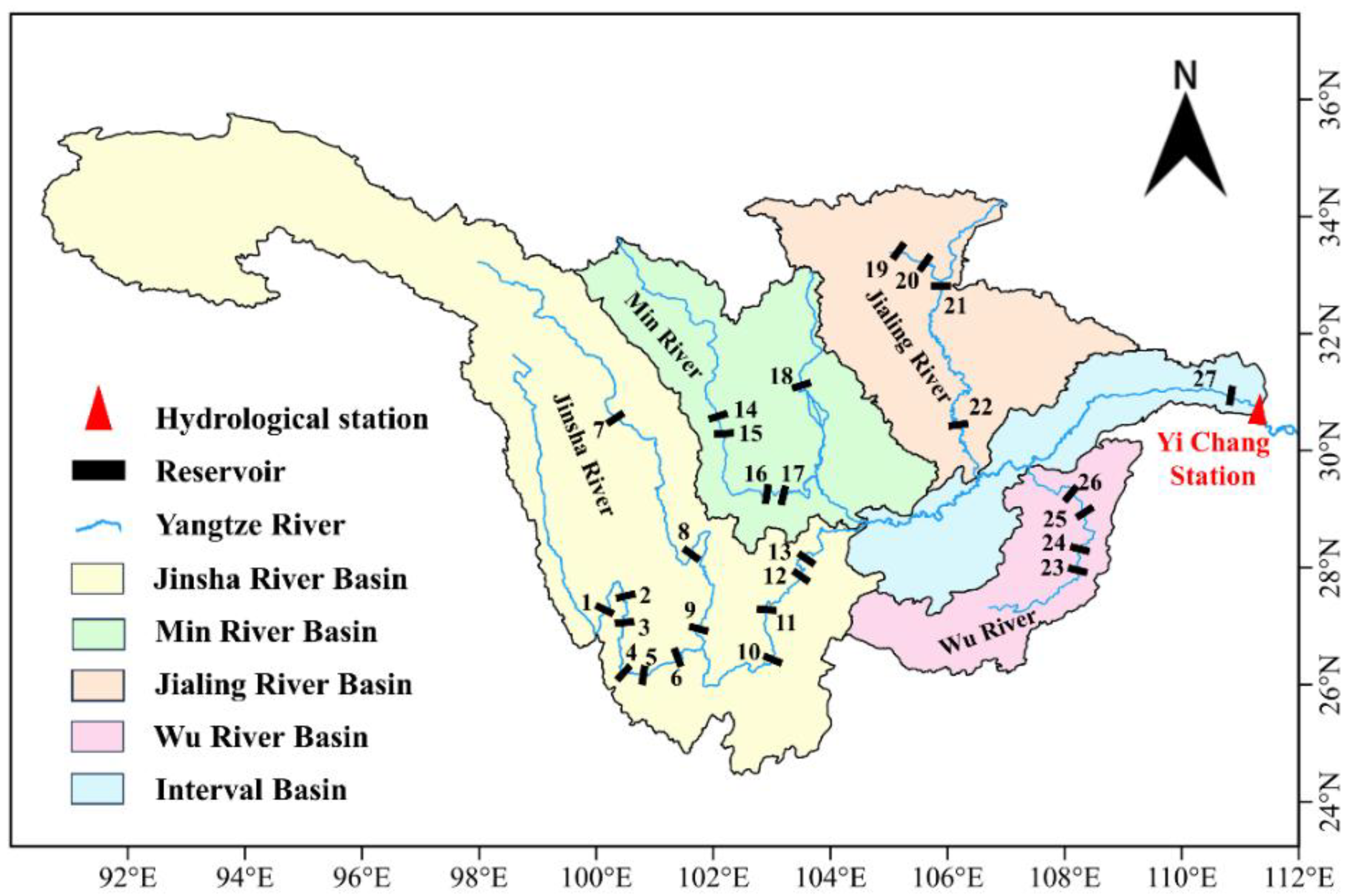
Figure 1. Locations of the key large-scale reservoirs in the upper Yangtze River basin. The numbers correspond to the reservoir numbers listed in Table 1.
Hydrology 12 00258 g001
Figure 2. The flowchart of the study.
Hydrology 12 00258 g002
Figure 3. The seasonal P-III frequency curves in the transition period from 1 August to 10 September.
Hydrology 12 00258 g003
Figure 4. Temporal dynamics of the seasonal maximum flood data series in the transition period from 1990 to 2022.
Hydrology 12 00258 g004
Figure 5. The MRI for the key large-scale reservoirs in the upper Yangtze River basin since the 1990s.
Hydrology 12 00258 g005
Figure 6. The Q-Q plot for the flood data series in the TGR transition period from 1 August to 10 September.
Hydrology 12 00258 g006
Figure 7. The centile plot for the flood data series in the TGR transition period from 1 August to 10 September.
Hydrology 12 00258 g007
Figure 8. Comparison of stationary and nonstationary P-III flood frequency curves in the transition period from 1 August to 10 September.
Hydrology 12 00258 g008
Figure 9. Comparison of the 1000-year seasonal design flood hydrographs derived from both stationary and nonstationary methods in the transition period from 1 August to 10 September.
Hydrology 12 00258 g009
Table 1. List of the characteristic parameters of the 27 key large-scale reservoirs in the upper Yangtze River basin.
BasinReservoir
Name
Reservoir NumberCatchment Area
(104 km2)
Flood Prevention Storage
Capacity (108 m3)
Operation Year
Jinsha RiverLiyuan122.001.732016
Ahai223.542.152014
Jinanqiao323.741.582012
Longkaikou424.001.262014
Ludila524.735.642014
Guanyinyan625.652.532016
Lianghekou76.5720.02022
Jinping-Ⅰ810.2616.02014
Ertan911.649.001999
Wudongde1040.6124.42021
Baihetan1143.0375.02022
Xiluodu1245.4446.52014
Xiangjiaba1345.889.032014
Min
River
Houziyan145.400.682017
Changheba155.670.362017
Dagangshan166.270.822015
Pubugou176.857.302010
Zipingpu182.271.672006
Jialing RiverBikou192.601.031997
Baozhusi202.842.801998
Tingzikou216.1114.42014
Caojie2215.611.992011
Wu RiverGoupitan234.332.002009
Silin244.861.842010
Shatuo255.452.092013
Pengshui266.902.322009
Yangtze RiverTGR27100.0221.52003
Table 2. Statistical parameters and design floods of Three Gorges Reservoir in construction period.
Flood SeriesMeanCvCs/CvDesign Frequency
0.1%1%2%5%
Qm (m3/s)52,0000.21498,80083,90078,80072,300
W3d (108 m3)130.00.214247.0209.3197.5180.7
W7d (108 m3)275.00.193.5486.8420.8399.9368.5
W15d (108 m3)524.00.193.0911.8796.5757.5702.2
Table 3. Investigated historical floods of TGR in the transition period from 1 August to 10 September.
YearQm (m3/s)W3d (108 m3)W7d (108 m3)W15d (108 m3)
115392,800 (1)232.7 (1)475.3 (1)/
122796,300 (2)241.6 (2)492.5 (2)/
156093,600 (3)234.8 (3)479.2 (3)/
Note: The number in parentheses represents the descending rank order in seasonal maximum flood data series in the transition period.
Table 4. Seasonal design floods of TGR estimated by P3/CF model in the transition period from 1 August to 10 September.
Flood SeriesMeanCvCs/CvDesign Frequency
0.10%1%2%5%
Qm (m3/s)43,5000.293.098,30080,60074,90066,900
W3d (108 m3)1080.293.0244200186166
W7d (108 m3)2270.272.5477400374338
W15d (108 m3)4240.262.0847722680620
Table 5. Estimated parameters and test results in transition period from 1 August to 10 September.
Flood
Series
Estimated ParametersK-S
Test
SSDAIC
ω 10 ω 11 ω 20 ω 21 ω 30
Qm12,963.62−56,767.904231.56−12,844.307.140.971.94 × 1082034.90
W3d27.95−30.7910.86−32.747.270.701.37 × 103319.88
W7d47.22−85.4521.76−89.908.220.942.58 × 103418.90
W15d−5.06−310.7129.72−81.2514.450.901.47 × 104684.20
Table 6. Nonstationary seasonal design floods estimated by Tv-P3/CF model in the TGR transition period from 1 August to 10 September.
Flood
Variables
Statistical ParametersDesign Frequency
MeanCvCs0.10%1%5%
Qm (m3/s)35,8000.270.7575,800 (−22.9%)63,200 (−21.6%)53,300 (−20.3%)
W3d (108 m3)940.270.74198 (−18.9%)165 (−17.5%)139 (−16.3%)
W7d (108 m3)1860.270.70389 (−18.4%)325 (−18.8%)276 (−18.3%)
W15d (108 m3)3510.280.53726 (−14.3%)615 (−14.8%)525 (−15.3%)
Note: The percentages in parentheses indicate the reduction rates of the nonstationary design flood compared to the original design flood.
Table 7. Comparison of hydropower generation with different design schemes for TGR in the transition period from 1 August to 10 September.
Design SchemeFLWL/FCWL (m)Hydropower (Billion kW h)Increase Rate
Stationary annual design14513.807/
Stationary seasonal design14914.7626.92%
Nonstationary seasonal design15716.09516.57%
Disclaimer/Publisher’s Note: The statements, opinions and data contained in all publications are solely those of the individual author(s) and contributor(s) and not of MDPI and/or the editor(s). MDPI and/or the editor(s) disclaim responsibility for any injury to people or property resulting from any ideas, methods, instructions or products referred to in the content.