Article

Exploring Seasonality Indices for Low-Flow Analysis on Tibagi Watershed (Brazil)

by
Alexandre Sokoloski de Azevedo Delduque de Macedo
and
Michael Männich
*
Department of Environmental Engineering, Federal University of Paraná, Centro Politécnico, Curitiba 81531-980, PR, Brazil
*
Author to whom correspondence should be addressed.
Hydrology 2025, 12(1), 19; https://doi.org/10.3390/hydrology12010019
Submission received: 5 December 2024 / Revised: 26 December 2024 / Accepted: 6 January 2025 / Published: 17 January 2025
(This article belongs to the Section Statistical Hydrology)

Abstract

:
This study investigated the seasonality of low-flow discharges in the Tibagi watershed, Paraná, Brazil, through the analysis of three indices: Seasonality Ratio ( S R ), Seasonality Index ( S I ), and Seasonality Histogram ( S H ). The indices were computed and compared using previously calculated low-flow discharge data ( Q 95 ) and physiographic information on sub-watersheds. A ‘Seasonality Calendar’ was developed, illustrating the period and intensity of low-flow discharge occurrences in the watershed. The results indicate that, despite the watershed not presenting a strong seasonality, there is a tendency for low-flow discharges to concentrate in certain months, notably in August, September, and October. Spatial analysis reveals varied patterns with a certain trend of increased seasonality intensity (parameter r) towards downstream (north) and as the watershed area increases. These indices emerge as valuable tools for water resource management, aiding decision-making for allocation and hydrological regionalization, such as optimizing granting water resource distribution during dry seasons based on the identified low-flow patterns and establishing different reference low-flow values throughout the year.

1. Introduction

Low flows in streams and rivers are the result of a combination of meteorological processes (rainfall and evapotranspiration) and the dynamics of water storage in the catchment [1,2]. The study of low-flow discharges and their seasonal characteristics is of great importance to many areas related to water resources, as it represents a crucial decision-making tool in water resource management [1,3,4,5,6]. It is important in the calculation of surface water availability for water supply planning, design and waste load allocation, reservoir storage, irrigation, recreation, navigation, and conservation, and a widely used variable in hydrological modeling [1,2,6,7]. The analysis of the seasonality of low-flow discharge occurrences also proves to be an important factor for the government, as water rights permits (or granting) in surface water bodies are based on it [6,7]. Furthermore, understanding and knowledge of the distribution of hydrologically homogeneous regions in terms of minimum seasonality presents itself as an interesting tool for determining points of water use in water bodies (abstraction, effluent discharge) [7], especially in relation to agriculture, which accounts for 50% of the country’s water demands, representing the sector with the highest demand [8]. So, understanding the pattern of seasonal behavior and its intensity would help in mitigating damage to cultivation of crops and planning seeding throughout the years.
To quantify and analyze this seasonality, various indices have been developed, allowing for a more precise assessment of flow patterns over time. In this study, we focus on three main indices: Seasonality Ratio ( S R ), Seasonality Index ( S I ), and Seasonality Histogram ( S H ). These indices, widely utilized in previous studies [4,6,9,10,11,12,13], provide a robust comparison and analysis, allowing observation of the low-flow seasonality pattern in the watersheds and its temporal–spatial behaviors. In addition, these indices are used to characterize and identify hydrologically similar regions and correlate them with the hydroclimatological aspects of each region.
In Brazil, the standout study, similar to the others conducted, is that of [13]. Other studies on the seasonality of low flows, primarily for decision-making purposes such as water rights permits in the granting process, have been conducted by analyzing periods with different patterns of minimum flows and then examining the impact of the water balance with these seasonal flows [7,14,15,16,17,18,19,20]. In general, those researchers use seasonal reference low flow solely because their regions demand more water in certain periods of the year, without considering a temporal–hydrological approach that could be supplemented with seasonality indices [21].
The Tibagi watershed presents, in various regions, a considerable watershed commitment index (ICB), which represents an indicator of water stress, as discussed in the diagnosis by [22]. This raises questions about the reference flow methodology in Paraná and in Brazil, which is based only on the 95% exceedance probabilities throughout the entire historical series. Therefore, commitment indices such as the ICB, along with seasonality indices, can serve as tools to identify possible locations for the use of seasonal reference flows, as will be discussed throughout the text [22].
In this context, there are two important resolutions, such as CNRH n° 140/2012 and CNRH n° 141/2012, which provide autonomy to granting authorities to explicitly consider seasonal variation when significantly present [23,24]. Considering this, if significant seasonality is observed, seasonal reference low flows could be employed in decision-making processes, such as water granting and license process, endorsed by the Agência Nacional de Águas e Saneamento Básico (ANA) itself [25]. Thus, this study presents a different and new perspective in the Paraná state region, showcasing the application of these indices at the watershed scale to understand and analyze the seasonal behavior of low flows and to correlate it with local catchment and climatological aspects. These seasonality indices provide an interface application for water resource management, aiding decision-making for optimizing water resource distribution during dry seasons based on the identified low-flow patterns and establishing different reference low-flow values throughout the year.

2. Materials and Methods
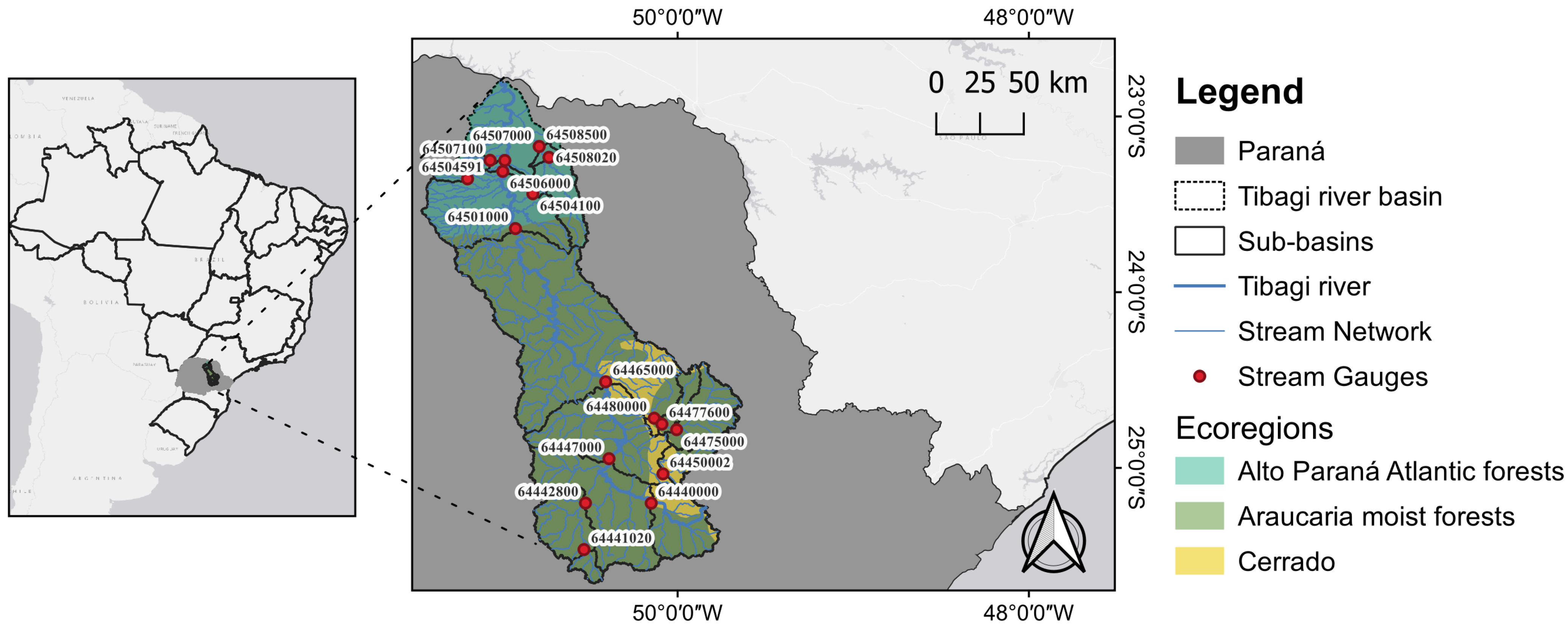
2.1. Study Area

This study was carried out in the Tibagir River watershed, which has a vast longitudinal extension, being one of the largest watersheds in the state of Paraná, Brazil, with a total area of 24 , 530 km 2 . The watershed is situated in the central-eastern portion of the state, and the main activity performed in the Tibagi River watershed is agriculture [22]. The Tibagi watershed shows a notably south–north orientation which encompasses three ecoregions, according to the classification in [26], which are the following: Alto Paraná Atlantic forests (Biome: Tropical and Subtropical Moist Broadleaf Forests), Araucanian moist forests (Biome: Tropical and Subtropical Moist Broadleaf Forests), and Cerrado (Biome: Tropical & Subtropical Grasslands, Savannas and Shrublands), as shown in Figure 1. Ecoregions represent the distribution of species and communities more accurately than maps derived from biophysical features [27]; however, they are also related to rainfall and temperature patterns. Agriculture, livestock, and forestry cover 73% of the watershed area; 25% is covered by forest and camps; and 1% is related to urban areas and other small sharing areas [28]. Additionally, the Tibagi River enters the Capivara Reservoir, which has a concern regarding phosphorus loading from its watershed [29].

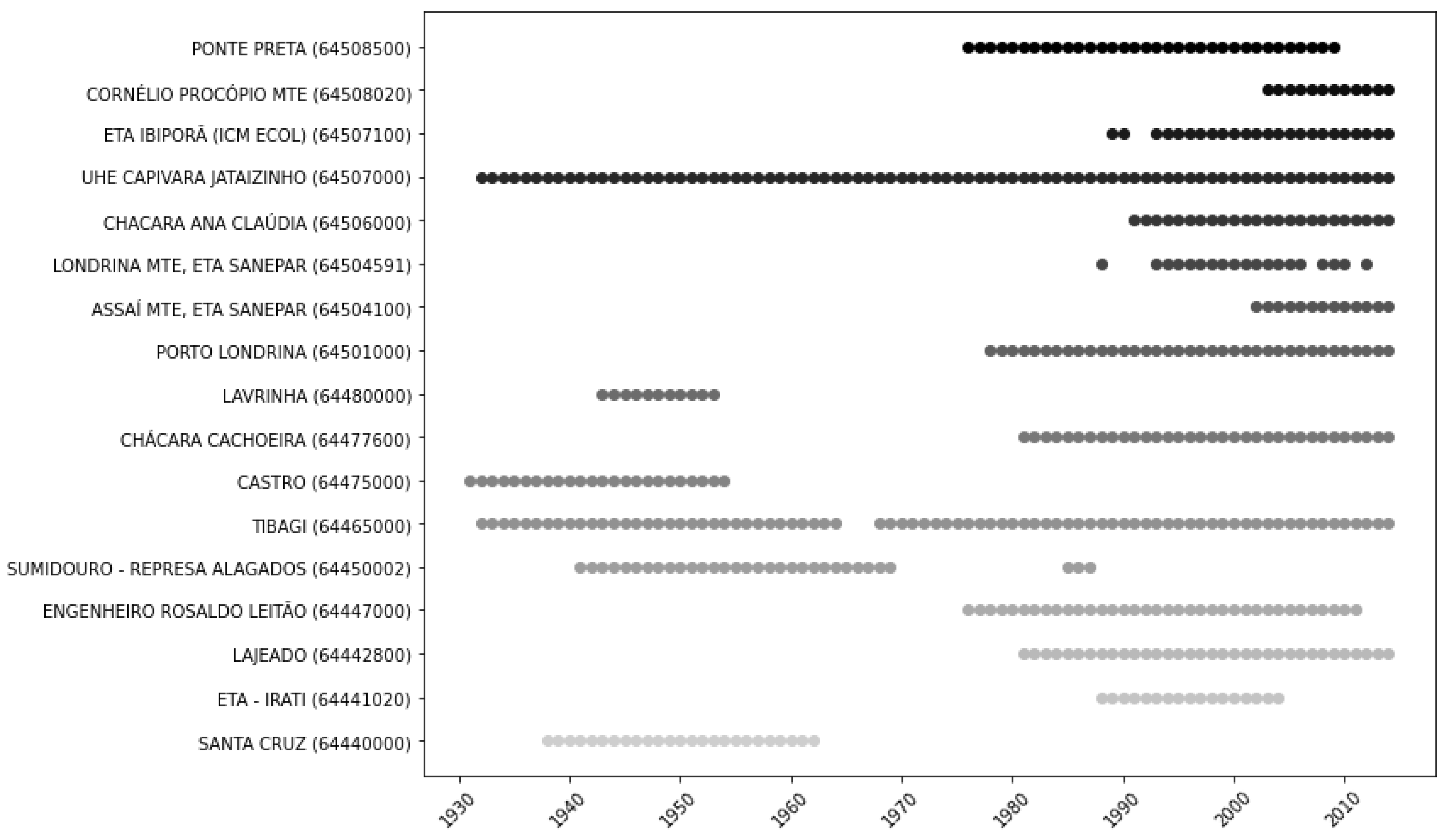
2.2. Data and Materials

The data for this study were obtained from the Hidroweb repository, maintained by ANA [30], resulting in 24 stream gauges with consistent data. We investigated stream gauges with at least 10 years of uninterrupted daily flow records, with less than 2 months of annual missing data. These selected thresholds aimed for the most extensive spatial coverage in the catchment, preserving the statistical representativeness of the low-flow calculation considering the minimum of 10 years of data [4]. Out of that, 17 stream gauges were retained for analysis, spanning from 1931 to 2014, and covering an area ranging from 29.7 to 21,938 km 2 , calculated using the Shuttle Radar Topography Mission (SRTM) shapefiles available in [31]. Figure 2 illustrates the available data periods of all stream gauges presented in Table 1.
To obtain the low-flow discharges, the series of daily mean flows were analyzed. The flow duration curves for each river gauging station were used to calculate the Q 95 values, which represent the flow equaling or exceeding 95% of the monitoring period.
The decision-making process in all Brazilian states relies on a percentage of low-flow reference values, as represented in Equation (1) [21]. These values determine the maximum legally granted water usage for each watershed user. This allocation remains constant throughout the year, with no explicit adjustments for seasonal variations, despite the existence of legal resolutions addressing seasonality [21]. The maximum water usage can be defined as
Q m a x = α · Q r e f ,
where Q m a x is the maximum legally granted flow rate, α is the permissible percentage to be allocated, and Q r e f is the respective low-flow reference value, different for each state [21].
In Brazil, Q 95 is the most commonly used reference for defining water rights permits. This includes its application in Paraná [32], including in the Tibagi watershed, and in 9 other states (out of 27) across the country. The parameter α ranges between 0.2 and 0.9 [21].

2.3. Seasonality Indices

The distribution of seasonality effects of low-flow discharges in the Tibagi watershed region and the identification of hydrologically homogeneous regions were evaluated through three seasonality indices: Seasonality Ratio ( S R ), Seasonality Index ( S I ), and Seasonality Histogram ( S H ).
The S R method, proposed by [12], involves dividing the series into two periods: a summer period and a winter period. The low-flow discharges were calculated for each of these periods. Subsequently, the minimum flows obtained from the partial series of summer periods ( Q 95 s ) are divided by the minimum flows obtained from the partial series of winter periods ( Q 95 w ). Thus, S R is represented by
S R = Q 95 s Q 95 w .
The presence of a winter low-flow regime is indicated when S R > 1 , and conversely, when S R < 1 , there is an indication of a summer regime. When S R = 1 , there is no indication of seasonality.
The S I method, proposed by [9], is used to express the seasonal distribution of low-flow discharge occurrences. The method involves the application of Equations (3) to (7) to obtain two main parameters: directional angle ( θ ) and mean vector length (r).
The directional angle θ represents the mean day of occurrence of low-flow discharges, expressed in radians. It is calculated by converting the day of the year into an angle, where θ = 0 corresponds to 1 January; θ = π / 2 to 1 April; θ = π to 1 July; θ = 3 π / 2 to 1 October; and θ = 2 π to 30 (or 31) December) (In normal years, days range from 1 to 365, but in leap years the range is from 1 to 366.).
The mean vector length r, also called the seasonal concentration index [6], is a dimensionless measure of the variability in low-flow occurrences. It ranges from 0 to 1, where r = 1 corresponds to strong seasonality (all low-flow events occur on the same day) and r = 0 indicates uniform distribution throughout the year.
The Seasonality Index takes into consideration the days when the flow was less than or equal to the low-flow discharge ( Q 95 ), which are transformed into Julian calendar dates ( D j ). Thus, the directional angle ( θ j ) in relation to D j is obtained as
θ j = 2 π 365 D j .
The arithmetic mean of the Cartesian coordinates x θ , y θ over a total of N days j is obtained by
x θ = 1 N j c o s ( θ j ) , and y θ = 1 N j s i n ( θ j ) .
θ is obtained by
θ = tan 1 y θ x θ , for the 1 st and 4 th quadrant , or θ = tan 1 y θ x θ + π , for the 2 nd and 3 rd quadrant .
The mean day of occurrence is obtained by transforming back θ into a Julian day, by
D = 365 2 π θ .
Finally, r is
r = x θ 2 + y θ 2 .
The third method is the S H , proposed by [11], which results in a seasonal histogram on a monthly scale. The S H allows for a more detailed description of the seasonal distribution of low-flow discharges than S I [12]. Again, based on the Julian calendar, the method counts the occurrences of flows lower than or equal to the low-flow discharge ( Q 95 of each stream gauge) in each month and provides complementary information to S I . Particularly, it indicates which months are affected by low-flow discharges and provides a good representation of the shape of the seasonal distribution, including multimodal and asymmetric distributions.

3. Results and Discussion

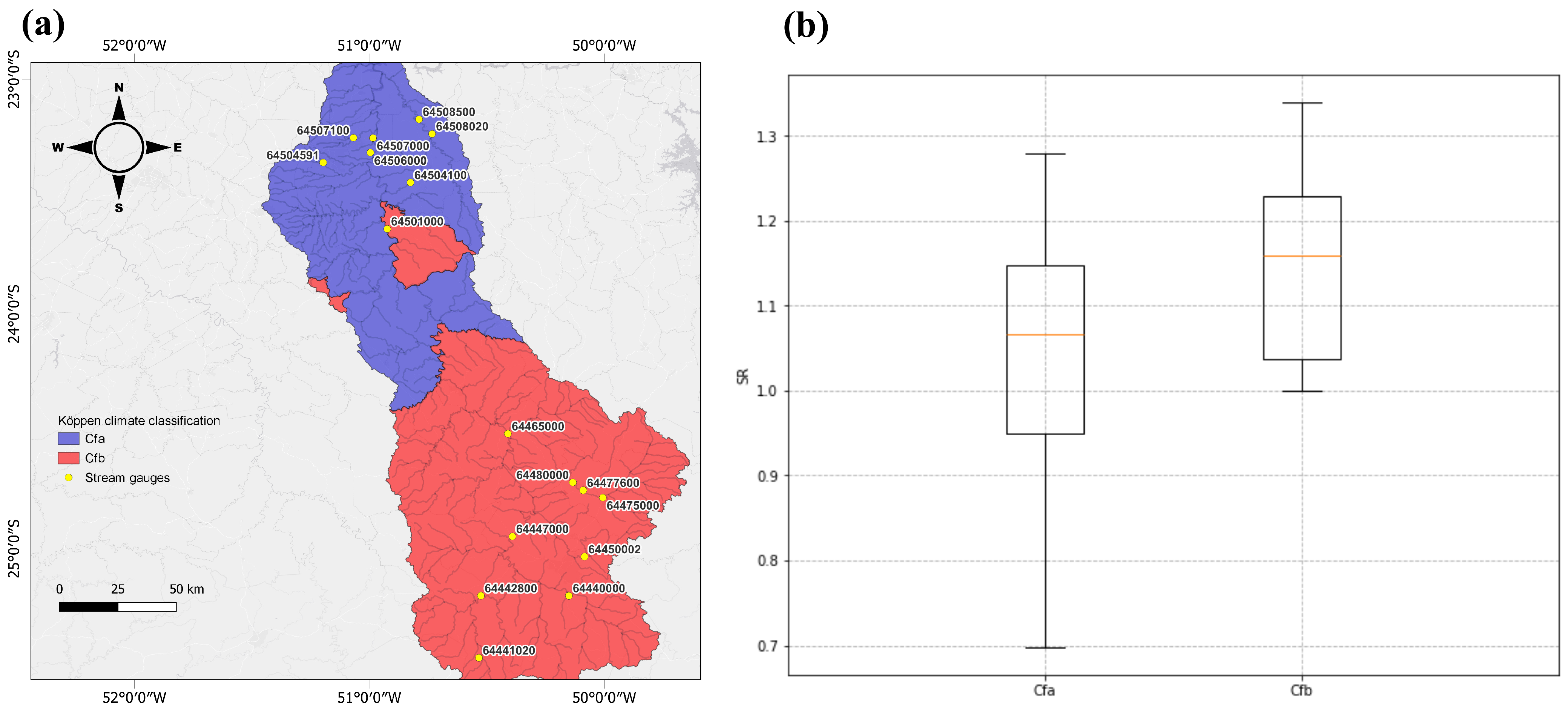
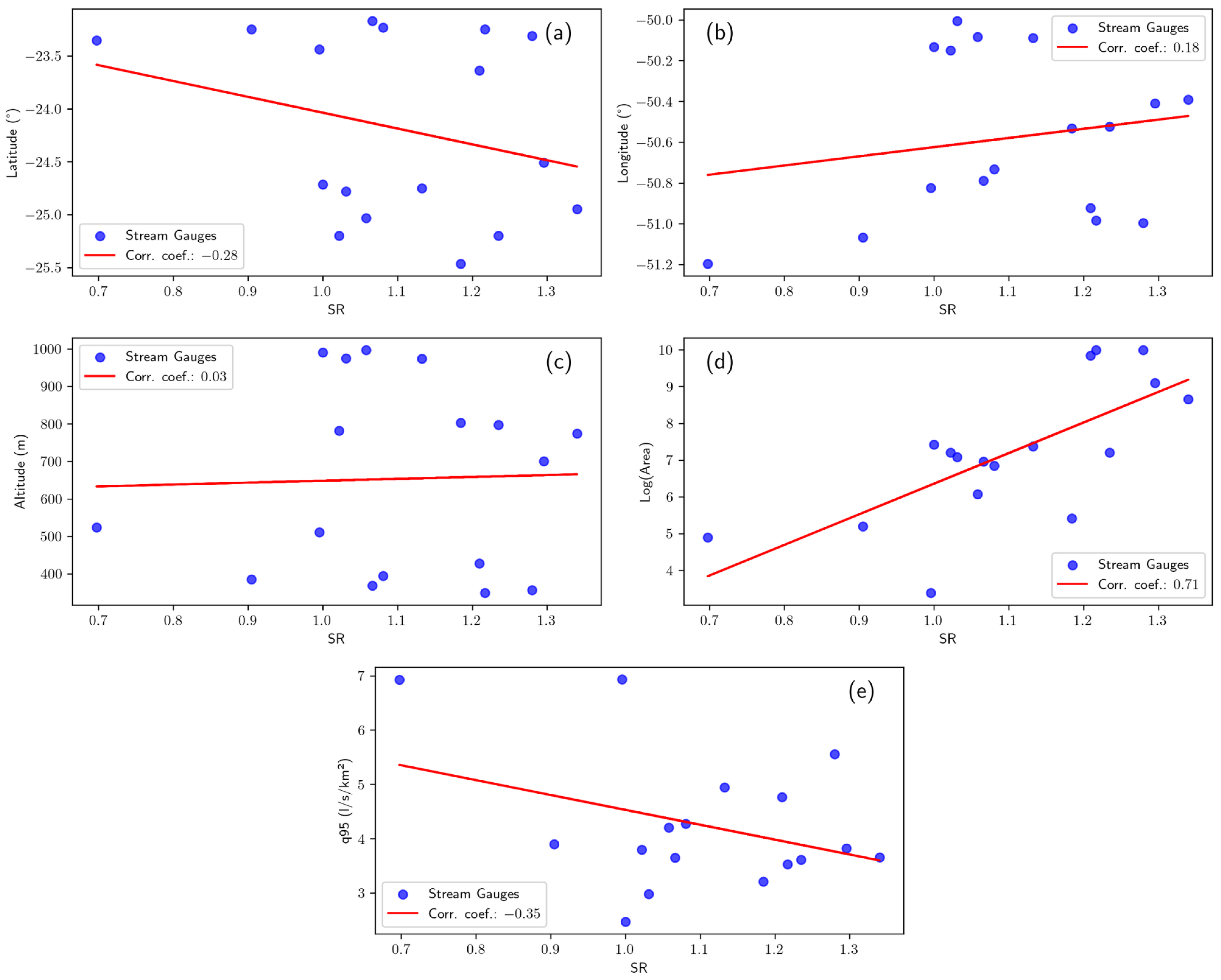
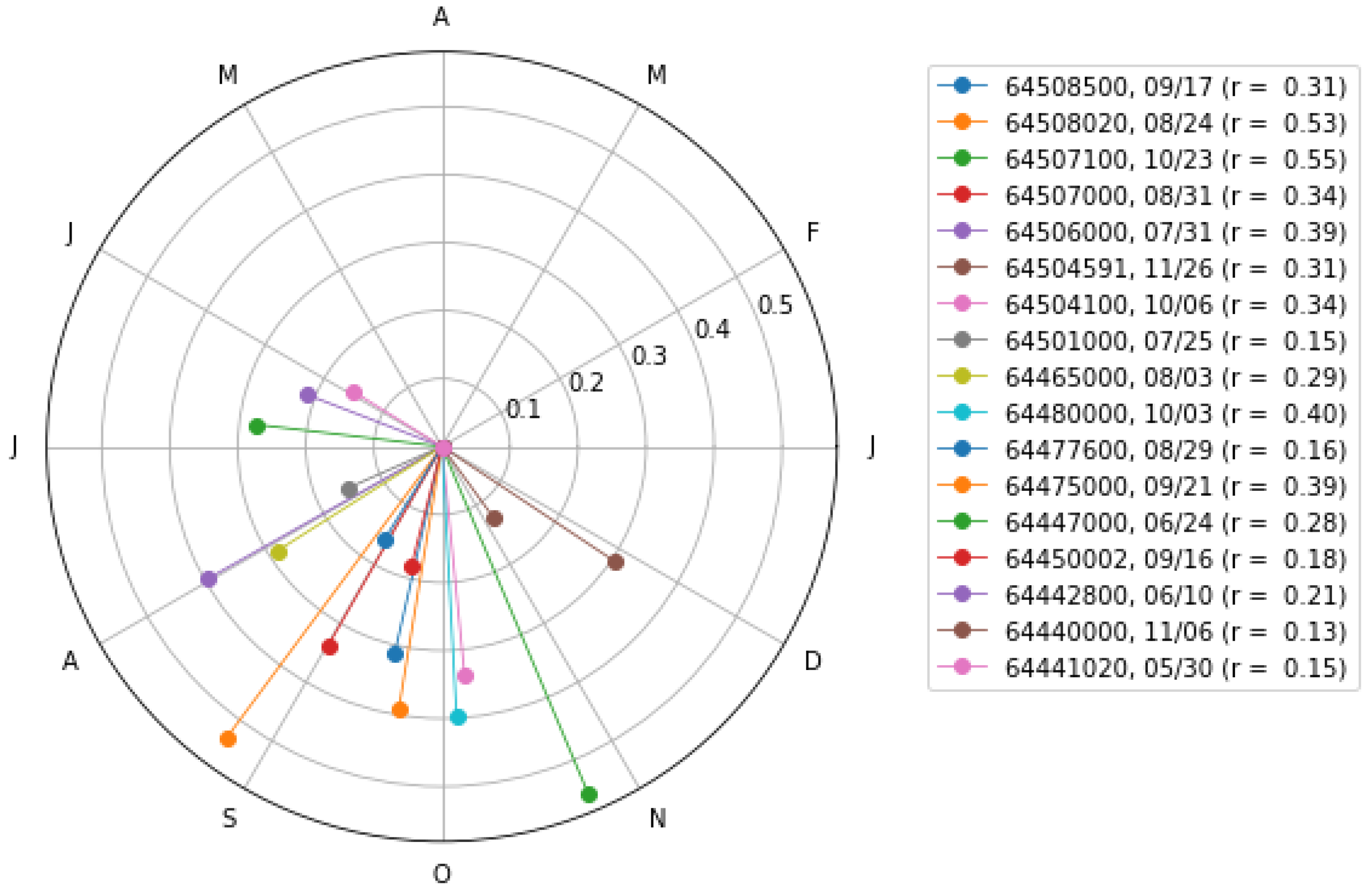
3.1. Seasonality Ratio

In the SR, as required by the index method, two periods were defined: winter (April to September) and summer (October to March), considering the driest and wettest periods in Paraná, respectively. The selection of these periods has also been used in other hydrological studies, such as the study conducted by [33]. The values of Q 95 w and Q 95 s are shown in Table 1.
The S R values found range from 0.7 to 1.3 and are spatially visualized in Figure 3. It is observed in Figure 3a that out of the 17 watersheds, 13 had S R > 1 and 4 watersheds had S R ≤ 1. Additionally, when classifying the watersheds into equally spaced intervals (as shown in Figure 3b) to better visualize the seasonality pattern, it can be seen that eight watersheds fall within the range of (1.1,1.3], eight watersheds fall between (0.9,1.1], and only one watershed falls in the range [0.7,0.9].
Although low-flow discharges are usually lower in winter, it is noted that the S R values, overall, are around 1.0, with an average and median of 1.1, indicating that there is not a significant difference, in most of the studied sub-watersheds, in summer and winter low-flow discharges. This is in line with the reference flow values (for both winter and summer periods) calculated and presented in Table 1.
This scenario differs from other watersheds, where low-flow values are influenced by distinct drivers, such as snow accumulation during winter and periods of high potential evapotranspiration exceeding precipitation during summer, as observed in European and North American watersheds [6,11,34]. As discussed by [34], in these regions, low flows mostly occur during winter in higher elevation regions, such as the European Alps, Scandinavia, the Rocky Mountains, and the Upper Midwest and Plains states, due to freezing temperatures that inhibit snowmelt. This contributes to a broader S R interval, contrasting with Southern Brazilian watersheds, as reported by [13], where the precipitation regime is more uniform throughout the year and there are no snowing conditions.
The S R values are consistent when considering the climatic characteristics of the state of Paraná, according to the Köppen classification [35]. The Tibagi river watershed is classified as Cfa (in the north) and Cfb (in the southern portion), as illustrated in the map in Figure 4a.
The Cfa classification indicates a humid subtropical climate with a tendency for rainfall concentration in the summer months but without a strictly defined dry season. On the other hand, Cfb represents a humid temperate climate, also without a clearly defined dry season throughout the year. Thus, the relatively homogeneous distribution of rainfall throughout the year is consistent with the S R values found, reflecting the expected pattern for these climatic classifications. The distribution of S R values throughout the basin can also be better visualized in Figure 4b for each Köppen classification. Higher values of S R are associated with the classification of the Cfb clime in the southern region of the watershed.
The S R values found by [13] in Rio Grande do Sul were also observed to be close to unity. This possibly occurred due to a well-distributed rainfall regime throughout the year, as also indicated by the Köppen classification (the same as the Tibagi watershed, Cfa/Cfb).
Ref. [11] found a strong relation between the altitude of the studied watersheds and their respective low-flow discharge values, which is reflected in the S R index. A distinct winter low-flow pattern is evident in Austrian watersheds at higher altitudes. This occurs due to rivers freezing during this period, resulting in river supply from snowmelt in spring and rainfall in summer.
Figure 5 explores the S R index correlation with physiographic aspects of the Tibagi watershed. No clear relation was identified between altitude and low-flow discharges. Similar results were found by [13]. However, according to Figure 5d there is a clear trend of increasing S R as the watershed increases, that is, it increases exponentially to the watershed area. That indicates a spatial scale effect on seasonality by catchment area.
Thus, as observed in the strong correlation shown in Figure 5d, the larger the log of the watershed area, the greater its tendency to have lower flow values during the winter period in the Tibagi watershed.

3.2. Seasonality Index

The Seasonality Index ( S I ) method aims to determine the mean day of occurrence of low-flow discharges D, and its respective seasonality intensity through the vector r, which is a measure of the variability in low-flow discharge seasonality, ranging from zero to one. One way to explore the S I method is the possibility of presenting the conventional hydrograph on a polar plot, in such a way that the days are transformed into angles, as indicated by Equation (3), and the days are plotted against the mean daily discharges, as illustrated in Figure 6. This representation becomes useful by treating time as a cyclical variable, especially when the aim is to visualize seasonal patterns, analyze shifts, and emphasize the low-flow or maximum discharges of a certain historical series or for a period, as represented in Figure 6b. It is evident that, for Station 64508020, the low-flow discharges are concentrated, mostly, in the second half of the year with D = 08 / 24 , as shown in Figure 7. This analysis is not so evident through visual inspection of the conventional hydrograph.
The S I index, by computing the values of θ and r for each of the stream gauges (according to Equations (5) and (7)), produces a ‘Seasonality Calendar’, as illustrated in Figure 7, which can be also interpreted as a mean value of the polar hydrograph.
The analysis of Figure 7 allows for extracting important information about the entire watershed. It reveals not only the dates on which low-flow discharge occurrences are concentrated but also their intensities. These pieces of information are visually represented by the mean day of occurrence vector (r). Thus, the Seasonality Calendar represents an effective graphical tool for observing and synthesizing the seasonality regime of a particular hydrographic watershed.
In the case of the Tibagi watershed, as represented in Figure 7, it is noticeable that the occurrences of low-flow discharges in 14 out of 17 stations in the watershed tend to concentrate in the second half of the year. This trend is not unique to discharge; according to the Climatic Atlas of Paraná of 2019 [36], similar seasonal patterns are observed in other climatological variables, such as precipitation and humidity, which also decrease during this period. Comparatively, temperate regions like Europe and North America exhibit distinct patterns, with low flows often occurring in winter due to snow-related processes [34]. Additionally, the intensity of this seasonality, represented by the r values, varies from 0.13 to 0.55, according to Table 2.
The values calculated in the S I index and its parameters are presented in Table 2 and are also spatially represented in Figure 8. The D values range from 150 to 330 (30 May to 26 November). As illustrated in Figure 8a, the Tibagi watershed exhibits a diverse distribution of the mean day (D) throughout the region, with an average occurrence in the watershed on 30 August. The smaller watersheds usually show a higher seasonality intensity. The southwestern part of the watershed shows an early mean day D, showing that the average day of occurrence is closer to the middle of the year, meaning in the middle of Paraná’s winter. In a non-leap year, following a conventional calendar, the data reveal the distribution in the Tibagi watershed according to Table 3. The results in the watershed corroborate the drought pattern described by [37].
In American and European regions, a distinct seasonal transition in flow patterns can be observed [34]. While [34] initially hypothesized that low flows would primarily be influenced by temperature variations (and closely linked to evapotranspiration), their findings revealed a different mechanism. In catchments experiencing winter low flows, the primary driver of the impact of rising temperatures on low flows was related to changes in snow dynamics, including accumulation and melting processes. Higher summer temperatures are expected to intensify soil moisture deficits, potentially causing reduced flows [38,39,40]. However, these temperature increases are unlikely to significantly alter the timing of low flows, as the peak temperatures—and consequently, the periods of highest excess potential evapotranspiration—are still projected to occur from mid- to late summer [34].
The scenario of non-uniform distribution of the parameter D indicates that in the Tibagi watershed there is not a strong and marked seasonality considering low flows. This observation becomes evident when analyzing the mean day intensity vector (r). However, it is possible to observe that the further downstream in the watershed, the greater the seasonality, as evidenced by Figure 9b, because the further north (higher latitude), the greater the r (correlation coefficient of 0.61).
However, as observed by [13], r values above 0.4 can be indicative of moderate to strong seasonality. Upon examining Figure 8b, it is noted that only two watersheds presented r values falling into this category, both located further downstream in the Tibagi watershed, in the northern part of the state.
This increased seasonality, evidenced by a more pronounced dry period, was discussed by [37], who demonstrated a more accentuated dry period in regions to the north of Paraná. This observation has also been highlighted by other studies such as [41,42], underlining that the northern part of the state is characterized by lower rainfall. Furthermore, Ref. [43] verified that the north and northwest regions of Paraná present a high risk of water scarcity.
Ref. [37] concluded that there were more droughts in Paraná State as one moved away from the ocean and the altitude of the state decreased, also indicating a higher seasonality. Moreover, Refs. [44,45] reported that the occurrence of dry periods is strongly associated with relief and maritime/continental influences, which in turn influence the air masses acting in each region. Similarly, regions with higher altitudes record higher rainfall indices throughout the year [37], leading to lower seasonality, as observed in Table 2 and Figure 8b.
Despite the relative increase in seasonality, it is important to emphasize that it remains low. This is because a significant portion of precipitation in the Tibagi watershed (70%) is influenced by atmospheric systems originating in the Amazon region [46], which promote a relatively uniform distribution of rainfall throughout the year, resulting in lower seasonality in the region [36]. This pattern is unique, as these atmospheric systems contribute to water abundance in the state of Paraná and rare occurrences of droughts throughout the year, as evidenced by the Seasonality Index.
The results of r and D are consistent with the observations of [33], who described the rainfall regime in the region as more uniform throughout the year in much of the Tibagi watershed, contrasting with less intense precipitation in the northern part, reflected in the more pronounced Seasonality Index. Moreover, the dry period, as described by [37], also confirms the behavior observed in Figure 8a.
Therefore, both r and D, the parameters associated with the S I index, can be used for characterizing the region and identifying hydrologically homogeneous areas (such as precipitation, altitude, and soil characteristics) in terms of the seasonality of minimum flows and can be adopted as criteria for the regionalization of minimum flows.
The S I index offers more detailed information than the S R index, as highlighted by [13]. Furthermore, the S I is not only valuable for assessing the seasonality of minimum flows but can also be employed in the analysis of the seasonality of flood flows, as indicated by [9,10,11,12].
The parameters of the S I method can also be applied for delineating hydrologically homogeneous regions considering the seasonality pattern. Its parameters (D and r) can offer important support in decision-making for water resource allocation, especially in contexts of water conflict and high criticality, as observed in various areas of the Tibagi watershed [47].
One possible application of the SI in decision-making could be the following: First, identifying regions with water conflicts or critical basin conditions, as demonstrated by [47], and then analyzing the distribution of R to assess basin seasonality and the average day of seasonality D, which could help evaluate the hydrograph of mean flows. Based on this analysis, a seasonal reference flow could be defined (e.g., ‘summer’ and ‘winter’) within the granted low-flow value, as shown in Equation (1). In this case, there would be two reference flow values for the basin, varying according to water availability, as current legislation already allows [23,24]. Finally, water allocation to users could be made more flexible by using seasonal reference flows, as highlighted by [21].

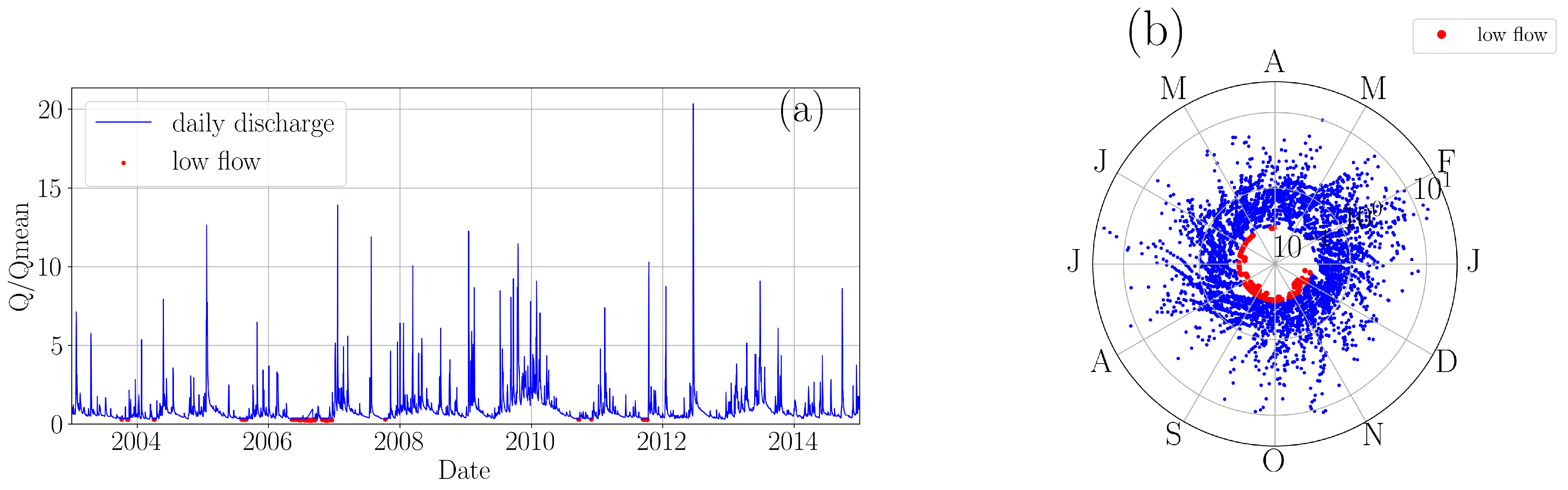
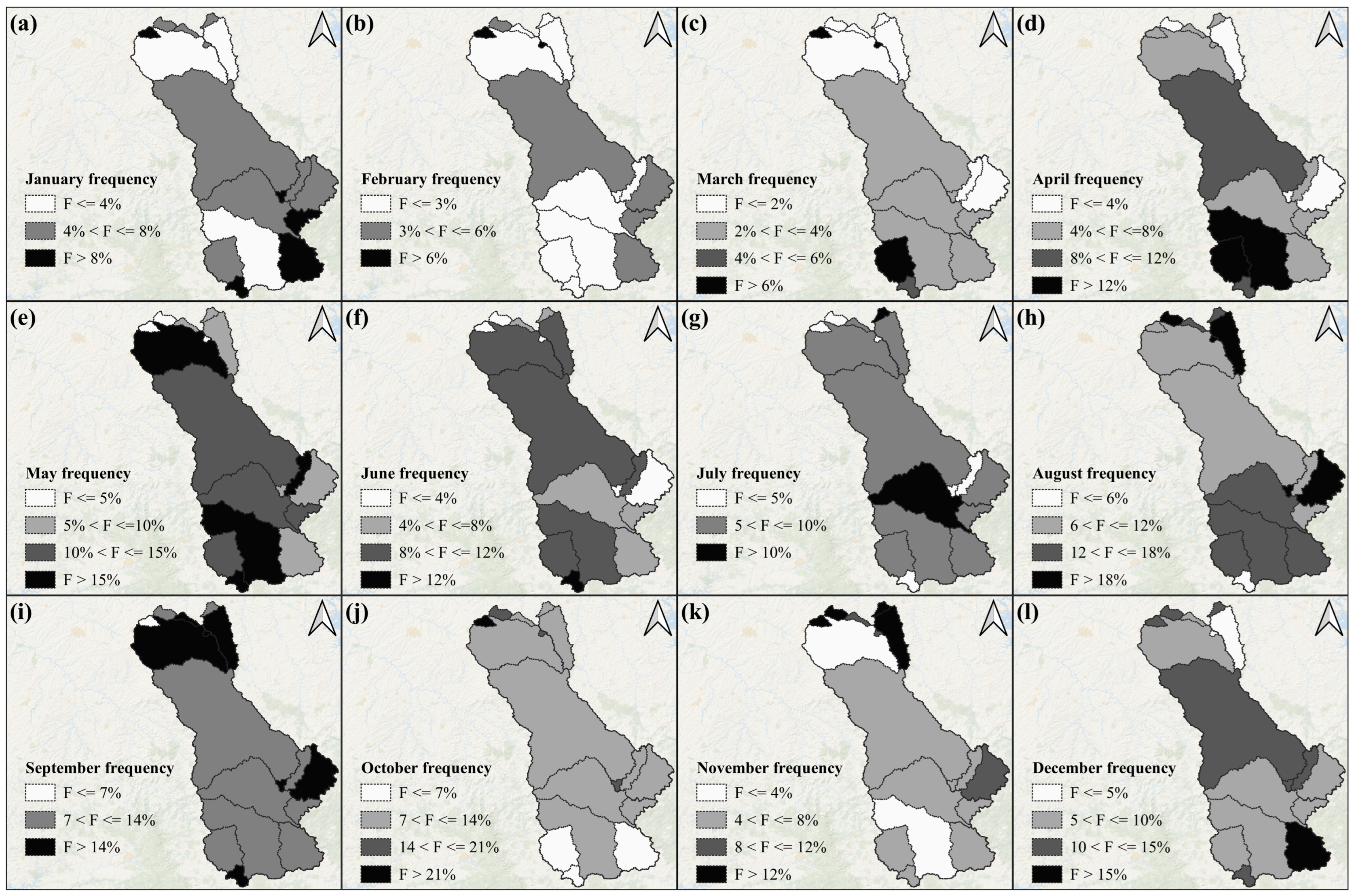
3.3. Seasonality Histogram

The S H method presents the occurrence of low flows for each month of the year, at all river gauge stations. These frequencies are presented in Figure 10. This method stands out for its richness of detail compared to the other two seasonality indices and can be seen as a more elaborate ‘synthesis’ of the other methods. Displaying the occurrence of events in each month of the year using 12 parameters allows for a more detailed and thorough analysis of the seasonal hydrological distribution of occurrences.
This monthly resolution enables the identification of specific trends and anomalies that broader indices might overlook. For example, the S H can reveal the behavior of multimodal distributions, indicating that low-flow events may occur across multiple months rather than concentrating in a single period. This is crucial for understanding hydrological patterns throughout the year. Such behavior is summarized in the low values of R, along the low-flow value concentrated in D. Moreover, the S H provides a more detailed view of months particularly vulnerable to low flows, offering valuable insights into potential water scarcity periods that may require targeted management strategies.
It is observed in Figure 10 that the months with the highest occurrences of low flows are August, September, and October, respectively. These values behave very similarly to those obtained by the D parameter in the S I index when observing the spatial distribution by regions.
Regarding water resource management in the Tibagi Basin, the S H index can be a powerful tool for assessing water availability on a monthly basis and optimizing resource use. The S H index enables the identification of regions with greater seasonality, while areas of higher criticality can be highlighted through the use of the watershed commitment index (ICB), similar to the water stress index (WSI), as demonstrated in the study by [47] for the Tibagi Basin itself. Thus, analyzing how seasonality influences relative flow gains during specific periods of the year becomes a promising approach to enhancing water resource management.
This information allows public authorities to focus efforts on investigating the feasibility of establishing a seasonal reference flow, thereby promoting more efficient water resource management. In this context, as discussed by [21], Equation (1) can be adapted to determine different Q r e f values throughout the year, adjusting to seasonal conditions (e.g., a monthly or six-month basis). This would enable users to strategically plan for the sustainable use of water resources, taking into account the hydrological characteristics of each period.

4. Conclusions

The Tibagi watershed generally exhibits weak seasonality in low flows, with the exception of two northern sub-watersheds where seasonality is moderate to strong, driven by stronger droughts. Among its sub-watersheds (only 2 out of 17 show r values above 0.4, and 0.7 < S R < 1.3 ), there is a tendency for low-flow concentrations during certain periods of the year, as indicated by the D parameter and better observed through the S H method, where the months of August, September, and October shown the highest occurrences of low flows, respectively.
The correlation between S R and the watershed area aligns with the water resource management organization in larger areas. Even small watersheds are more susceptible to water conflicts, and the larger ones exhibit higher seasonality in low flows. In this context, seasonality indices are a valuable alternative to guide decision-making, providing a deeper understanding of the spatial behavior of water availability, considering the reference flow for the water grant criteria of the state of Paraná, through Q 95 . These indices can be an important tool for companies and management agencies, such as for the licensing and granting process, when deciding on water intake locations (or dilution, in the case of effluent discharges), allowing for a more precise analysis of seasonal demands and the frequency of water resource use. Furthermore, the indices can be used as a basis for the use of seasonal reference flows, as already discussed by [25]. The additional results of this research can be a starting point for how seasonality can be included in water resource management, considering the lack of methodology in CNRH n° 140/2012 and CNRH n° 141/2012.
Moreover, the indices can be useful in defining homogeneous regions along with other relevant watershed characteristics (geography, altitude, etc.) regarding low flows, aiming for hydrological regionalization appropriately, and assisting water resource management in Paraná. We found a correlation of the Seasonality Index with the watershed area. The larger the area, the larger the S R we found, and the larger the S R , the lower the q 95 , suggesting a spatial scale dependence of the low flows on seasonality.
Despite methods like S I and S H standing out as the best options for describing hydrological regions’ seasonally and assisting in water resource management, including licensing and the application of seasonal reference flows when necessary, the S R method also proves to be a useful alternative. It can provide an initial analysis of differences between rainy and dry periods of the year, offering important insights for subsequent analyses.
Future research on this topic could address a large dataset to determine seasonality patterns across Brazil resulting from meteorological drivers and catchment storage dynamics based on the approach in [2], including how seasonality patterns interact with anthropogenic influences such as changes in land use or water withdrawals. Furthermore, by identifying regions of higher seasonality, benefits can be gained from using seasonal reference flow to define water rights.

Author Contributions

A.S.d.A.D.d.M.: writing—original draft, editing, visualization, methodology, formal analysis, data curation, conceptualization, software; M.M.: conceptualization, methodology, project administration, supervision. All authors have read and agreed to the published version of the manuscript.

Funding

This research received no external funding.

Data Availability Statement

All discharge data were obtained from the Agência Nacional de Águas e Saneamento Básico (ANA) through the Hidroweb portal, an online platform, and are publicly available.

Conflicts of Interest

The authors declare no conflicts of interest.

References

  1. Smahtin, V.U. Low flow hydrology: A review. J. Hydrol. 2001, 240, 147–186. [Google Scholar] [CrossRef]
  2. Chagas, V.B.; Chaffe, P.L.; Bloschl, G. Regional low flow hydrology: Model development and evaluation. Water Resour. Res. 2024, 60, e2023WR035063. [Google Scholar] [CrossRef]
  3. Schreiber, P.; Demuth, S. Regionalization of low flows in southwest Germany. Hydrol. Sci. J. 1997, 42, 845–858. [Google Scholar] [CrossRef]
  4. Vezza, P.; Rosso, M.; Viglione, A.; Claps, P. Low flows regionalization in north-western Italy. Water Resour. Manag. 2010, 24, 4049–4074. [Google Scholar] [CrossRef]
  5. Pruski, F.F.; Braga, C.C.; Nascimento, A.D.; Ramos, M.M. Low-flow estimates in regions of extrapolation of the regionalization equations: A new concept. Eng. Agric. 2015, 35, 808–816. [Google Scholar] [CrossRef]
  6. Cupak, A.; Kaczor, G. Determination of seasonal indices for the regionalization of low flows in the upper Vistula River Basin. Water 2023, 15, 246. [Google Scholar] [CrossRef]
  7. Serrano, L.D.O.; Ribeiro, R.B.; Borges, A.C.; Pruski, F.F. Low-Flow Seasonality and Effects on Water Availability throughout the River Network. Water Resour. Manag. 2020, 34, 1289–1304. [Google Scholar] [CrossRef]
  8. ANA. Conjuntura dos Recursos Hídricos no Brasil 2021: Informe Anual; ANA: Brasília, Brazil, 2021. [Google Scholar]
  9. Burn, D.H.; Zrinji, Z.; Kowalchuk, M. Regionalization of catchments for regional flood frequency analysis. J. Hydrol. Eng. 1997, 2, 76–82. [Google Scholar] [CrossRef]
  10. Young, A.; Round, C.; Gustard, A. Spatial and temporal variations in the occurrence of low flow events in the UK. Hydrol. Earth Syst. Sci. 2000, 4, 35–45. [Google Scholar] [CrossRef]
  11. Laaha, G. Modelling summer and winter droughts as a basis for estimating river low flows. In FRIEND 2002—Regional Hydrology: Bridging the Gap Between Research and Practice; van Lanen, H.A.J., Demuth, S., Eds.; IAHS Publication No. 274; IAHS Press: Wallingford, UK, 2002; pp. 289–295. [Google Scholar]
  12. Laaha, G.; Bloschl, G. Seasonality indices for regionalizing low flows. Hydrol. Process. Int. J. 2006, 20, 3851–3878. [Google Scholar] [CrossRef]
  13. Beskow, S.; Mello, C.R.; Faria, L.C.; Fernandes, M.M.; Viola, M.R. Índices de sazonalidade para regionalização hidrológica de vazões de estiagem no Rio Grande do Sul. Rev. Bras. Eng. Agric. Ambient. 2014, 18, 748–754. [Google Scholar] [CrossRef]
  14. Euclides, H.P.; Ferreira, P.A.; Filho, R.F. Critério de outorga sazonal para a agricultura irrigada no estado de Minas Gerais–estudo de caso. Rev. Item–Irrig. Tecnol. Mod. 2006, 71/72, 42–50. [Google Scholar]
  15. Silva, D.D.D.; Marques, F.A.; Lemos, A.F. Flexibilidade das vazões mínimas de referência com a adoção do período trimestral. Rev. Eng. Agric. 2011, 19, 244–254. [Google Scholar] [CrossRef]
  16. Bof, L.H.N.; Silva, D.D.; Mello, C.R.; Viola, M.R. Analysis of appropriate timescales for water diversion permits in Brazil. Environ. Manag. 2013, 51, 492–500. [Google Scholar] [CrossRef] [PubMed]
  17. Silva, B.M.B.d.; Silva, D.D.d.; Moreira, M.C. Influência da sazonalidade das vazões nos critérios de outorga de uso da água: Estudo de caso da bacia do rio Paraopeba. Rev. Ambiente Água 2015, 10, 623–634. [Google Scholar]
  18. Ribeiro, T.B.; Santos, P.C.P.; Pires, G.V.; Brito, A.O. Estimativa das vazões mínimas de referência (Q7,10, Q95 e Q90) anuais e semestrais para a bacia do rio Branco. In Proceedings of the XXII Simpósio Brasileiro de Recursos Hídricos, Florianópolis, Brazil, 26 November–1 December 2017. [Google Scholar]
  19. Arai, F.K.; Santos, L.G.; Silva, M.R.; Paz, A.R. Seasonality and criteria for concession of water in the Ivinhema basin. Res. Soc. Dev. 2020, 9, e1969108391. [Google Scholar] [CrossRef]
  20. Moreira, H.S.; Silva, D.D.; Prado, R.B.; Moreira, M.C. Cenários de disponibilidade hídrica para concessão de outorga: Estudo de caso da bacia Vertentes do Rio Grande, estados de Minas Gerais e São Paulo, Brasil. Rev. Bras. Gestão Ambient. Susten. 2020, 7, 341–350. [Google Scholar] [CrossRef]
  21. Macedo, A.S.A.D.; Stinghen, C.M.; Mannich, M. Vazões de referência sazonal e sua aplicação na outorga de recursos hídricos. Rev. Gestão Água Am. Lat. 2024, 21, e21. [Google Scholar] [CrossRef]
  22. Mannich, M.; Stinghen, C.M. Diagnóstico de outorgas de captação e lançamento de efluentes no Paraná e impactos dos usos insignificantes. Rev. Gestão Água Am. Lat. 2019, 16, e10. [Google Scholar] [CrossRef]
  23. CNRH. Resolução CNRH Nº 140, de 21 de Março de 2012. In Estabelece Critérios Gerais para Outorga de Lançamento de Efluentes com fins de Diluição em Corpos de Água Superficiais; Publicada no D.O.U. em 22/08/2012; CNRH: Brasília, Brazil, 2012. [Google Scholar]
  24. CNRH. Resolução CNRH Nº 141, de 10 de Julho de 2012. In Estabelece Critérios e Diretrizes para Implementação dos Instrumentos de Outorga de Direito de uso de Recursos Hídricos e de Enquadramento dos corpos de Água em Classes, Segundo os usos Preponderantes da Água, em rios Intermitentes e Efêmeros, e dá Outras Providências; Publicada no D.O.U. em 24/08/2012; CNRH: Brasília, Brazil, 2012. [Google Scholar]
  25. ANA. Outorga com Gestão de Garantia e Prioridade (OGP)—Uma Proposta para Maximização do uso da Água. 2022. Available online: https://participacao-social.ana.gov.br/api/files/Parecer_Tecnico_3_2022_SRE-1675339471836.pdf (accessed on 22 March 2024).
  26. Dinerstein, E.; Olson, D.; Joshi, A.; Vynne, C.; Burgess, N.D.; Wikramanayake, E.; Hahn, N.; Palminteri, S.; Hedao, P. An ecoregion-based approach to protecting half the terrestrial realm. BioScience 2017, 67, 534–545. [Google Scholar] [CrossRef]
  27. Olson, D.M.; Dinerstein, E.; Wikramanayake, E.D.; Burgess, N.D.; Powell, G.V.; Underwood, E.C.; D’Amico, J.A.; Itoua, I.; Strand, H.E.; Morrison, J.C.; et al. Terrestrial ecoregions of the world: A new map of life on earth: A new global map of terrestrial ecoregions provides an innovative tool for conserving biodiversity. BioScience 2001, 51, 933–938. [Google Scholar] [CrossRef]
  28. ANA. Comitê da Bacia Hidrográfica Rio Paranapanema—CBHRP. Plano Integrado de Recursos Hídricos da Unidade de Gestão de Recursos Hídricos Paranapanema; ANA/CBHRP: Brasília, Brazil, 2016. [Google Scholar]
  29. Porras, E.A.A.; Santos, J.G.; Borges, M.A.; Pereira, L.C.; Souza, L.T. Modelo de estimativa de cargas de fósforo como auxílio na gestão da bacia hidrográfica do rio Tibagi. In Proceedings of the XXIV Simpósio Brasileiro de Recursos Hídricos, Porto Alegre, Brasil, 21–26 November 2021; pp. 1–9. Available online: https://anais.abrhidro.org.br/job.php?Job=13605 (accessed on 14 April 2023).
  30. Hidroweb—Sistema de Informações Hidrológicas. 2023. Available online: https://www.snirh.gov.br/hidroweb/download (accessed on 17 July 2023).
  31. INPE. TOPODATA: Banco de dados Geomorfológicos do Brasil. 2011. Available online: http://www.dsr.inpe.br/topodata/data/geotiff/?C=N;O=D (accessed on 25 July 2023).
  32. SUDERHSA. Manual Técnico de Outorgas, Revision 01; Superintendência de Desenvolvimento de Recursos Hídricos e Saneamento Ambiental—DEOF: Paraná, Brazil, 2006. Available online: https://www.iat.pr.gov.br/sites/agua-terra/arquivos_restritos/files/documento/2020-10/manual_outorgas_suderhsa_2006.pdf (accessed on 7 January 2025).
  33. Nery, J.T.; Vargas, W.M.; Martins, M. Caracterização da precipitação no estado do Paraná. Rev. Bras. Agrometeorol. 1996, 4, 81–89. [Google Scholar]
  34. Floriancic, M.G.; Berghuijs, W.R.; Molnar, P.; Kirchner, J.W. Seasonality and drivers of low flows across Europe and the United States. Water Resour. Res. 2021, 57, e2019WR026928. [Google Scholar] [CrossRef]
  35. Parolin, M.; Volkmer-Ribeiro, C.; Leandrini, J.A. Abordagem Ambiental Interdisciplinar em Bacias Hidrográficas no Estado do Paraná; Editora da Fecilcam: Campo Mourão, Brazil, 2010. [Google Scholar]
  36. Nitsche, P.R.; Caramori, P.H.; Ricce, W.S.; Pinto, L.F.D. Atlas Climático do Estado do Paraná; IAPAR: Londrina, Brazil, 2019. [Google Scholar]
  37. Salton, F.G.; Morais, H.; Lohmann, M. Períodos secos no estado do Paraná. Rev. Bras. Meteorol. 2021, 36, 295–303. [Google Scholar] [CrossRef]
  38. Mastrotheodoros, T.; Pappas, C.; Molnar, P.; Burlando, P.; Manoli, G.; Parajka, J.; Rigon, R.; Szeles, B.; Bottazzi, M.; Hadjidoukas, P.; et al. More green and less blue water in the Alps during warmer summers. Nat. Clim. Change 2020, 10, 155–161. [Google Scholar] [CrossRef]
  39. Seneviratne, S.I.; Lehner, I.; Gurtz, J.; Teuling, A.J.; Lang, H.; Moser, U.; Grebner, D.; Menzel, L.; Schroff, K.; Vitvar, T.; et al. Swiss prealpine Rietholzbach research catchment and lysimeter: 32 year time series and 2003 drought event. Water Resour. Res. 2012, 48. [Google Scholar] [CrossRef]
  40. Teuling, A.J.; Van Loon, A.F.; Seneviratne, S.I.; Lehner, I.; Aubinet, M.; Heinesch, B.; Bernhofer, C.; Grünwald, T.; Prasse, H.; Spank, U. Evapotranspiration amplifies European summer drought. Geophys. Res. Lett. 2013, 40, 2071–2075. [Google Scholar] [CrossRef]
  41. Costa, A.B.F.D.; Santos, J.R.D.; Ferreira, L.C.; Alves, P.S.; Silva, M.E.A. Análise climatológica de dias consecutivos sem chuva no estado do Paraná. In Proceedings of the III Simpósio Internacional de Climatologia, Sociedade Brasileira de Meteorologia, Canela, Brazil, 18–21 October 2009. [Google Scholar]
  42. Fritzsons, E.; Vieira, M.L.; Amorim, R.; Franz, G.C.; Dias, G.A.R. Análise da pluviometria para definição de zonas homogêneas no estado do Paraná. RA’E GA—O Espaço Geogr. Anal. 2011, 23, 555–572. [Google Scholar]
  43. Wrege, M.S.; Steinmetz, S.; Reisser, C.; Almeida, I.R. Risco de deficiência hídrica na cultura do milho no estado do Paraná. Pesqui. Agropecu. Bras. 1999, 34, 1119–1124. [Google Scholar] [CrossRef]
  44. Vanhoni, F.; Mendonça, F. O clima do litoral do estado do Paraná. Rev. Bras. Climatol. 2008, 3, 49–63. [Google Scholar] [CrossRef]
  45. Mendonça, F.; Danni-Oliveira, I.M. Climatologia: Noções Básicas e Climas do Brasil; Oficina de Textos: São Paulo, Brazil, 2017. [Google Scholar]
  46. Van der Ent, R.J.; Savenije, H.H.; Schaefli, B.; Steele-Dunne, S.C. Origin and fate of atmospheric moisture over continents. Water Resour. Res. 2010, 46. [Google Scholar] [CrossRef]
  47. Stinghen, C.M.; Carvalho, J.M.; Mannich, M. Aplicação de indicador de estresse hídrico na bacia do rio Tibagi para a identificação de bacias críticas quanto ao uso dos recursos hídricos. Revista Gestão Água Am. Lat. 2022, 19, 2022. [Google Scholar] [CrossRef]
Figure 1. Locations of ecoregions and stream gauges present in the Tibagi watershed [26].
Hydrology 12 00019 g001
Figure 2. Stream gauges and their respective periods of data availability. Each circle corresponds to a single year of data.
Hydrology 12 00019 g002
Figure 3. Spatial distribution of Seasonality Ratio ( S R ) in the studied sub-watersheds. (a) Organized into two classes of S R greater and lower than 1, and (b) organized into three classes to highlight the differences.
Hydrology 12 00019 g003
Figure 4. (a) Köppen climatic classification, and (b) boxplot of Seasonality Ratio ( S R ) values found using the Köppen climatic classification class in the Tibagi watershed. The upper and lower limits of the boxes represent the 75th and 25th percentiles, respectively. The whiskers show the maximum and minimum values, and the red line represents the median.
Hydrology 12 00019 g004
Figure 5. Regression and correlation analysis of physiographic aspects in the Tibagi watershed, between Seasonality Ratio ( S R ) and (a) latitude, (b) longitude, (c) altitude, (d) drainage area, (e) normalized low flow (by area).
Hydrology 12 00019 g005
Figure 6. (a) Normalized hydrograph and (b) normalized polar hydrograph of flows normalized by the mean (Q/Qmean), from 2003 to 2014, for station 64508020. Flows equal to or less than the annual Q 95 are the low-flow discharges of the station, indicated by red dots.
Hydrology 12 00019 g006
Figure 7. Average occurrence of low-flow discharges, in terms of mean day ( θ ) and length of the mean vector (r), for the stream gauges of the Tibagi watershed. Each station is represented by one color. The length of the line represents the magnitude of the mean vector r in the polar coordinates.
Hydrology 12 00019 g007
Figure 8. Spatial distribution of (a) mean day (D) of occurrence of low-flow events in the 17 sub-watersheds studied, and (b) length of the mean vector (r).
Hydrology 12 00019 g008
Figure 9. Regression and correlation analysis of physiographic aspects in the Tibagi River watershed, between latitude and (a) mean day (D) and r between (b) latitude, (c) altitude, (d) drainage area, and (e) normalized low flow (by area).
Hydrology 12 00019 g009
Figure 10. Spatial distribution of Seasonality Histogram ( S H ), representing the occurrence of flows equal to or less than Q 95 in the Tibagi sub-watersheds, in the months of (a) January, (b) February, (c) March, (d) April, (e) May, (f) June, (g) July, (h) August, (i) September, (j) October, (k) November, and (l) December.
Hydrology 12 00019 g010
Table 1. Stream gauge information in the Tibagi watershed, for the period of available data (1931–2014).
Gauge (ID)Longitude (°)Latitude (°)Area ( km 2 ) Q 95 ( m 3 / s ) Q 95 w ( m 3 / s ) Q 95 s ( m 3 / s )Altitude (m)
64508500−50.788−23.17010493.8313.7333.980368.5
64508020−50.733−23.2329424.0264.0264.350394.3
64507100−51.068−23.2491810.7060.7460.675384.8
64507000−50.984−23.25021,93877.35671.46786.953349.5
64506000−50.995−23.31221,826121.306108.200138.466356.6
64504591−51.196−23.3541340.9281.1240.784524.1
64504100−50.824−23.43929.70.2060.2070.206510.8
64501000−50.923−23.63718,75889.40183.944101.538427.8
64465000−50.410−24.509166534.10430.83139.945700.3
64480000−50.133−24.71715934.1104.1104.110990.6
64477600−50.089−24.75011907.8807.3378.309973.9
64475000−50.006−24.78289293.5503.5503.660974.7
64447000−50.391−24.94743320.94118.78625.174774.8
64450002−50.083−25.03357311.8201.7201.820997.3
64442800−50.525−25.19913424.8504.5215.583797.1
64440000−50.150−25.2002255.1004.9905.100781.6
64441020−50.533−25.46413440.7220.6730.797803.2
The data include Q 95 (minimum flow with 95% exceedance probability), Q 95 w (wet season), and Q 95 s (dry season).
Table 2. Results obtained by the S I method for all stream gauges.
GaugesrDMean Day (mm/dd)
645085000.31260.709/17
645080200.53236.808/24
645071000.55296.910/23
645070000.34243.608/31
645060000.39212.407/31
645045910.31330.911/26
645041000.34279.510/06
645010000.15206.607/25
644650000.29215.308/03
644800000.40276.910/03
644776000.16241.608/29
644750000.39264.309/21
644470000.28175.706/24
644500020.18259.209/16
644428000.21161.206/10
644400000.13310.211/06
644410200.15150.205/30
The columns show the correlation coefficient (r), number of days (D), and mean day of occurrence in the format mm/dd.
Table 3. Distribution of the values of mean day (D) of occurrence of low-flow discharges in the Tibagi River watershed.
Mean DayOccurrence (%)
28 August–27 September29.4%
27 September–27 October17.6%
30 May–29 June17.6%
29 July–28 August17.6%
27 October–26 November11.8%
29 June–29 July5.9%
The table shows the periods of mean day (D) occurrence and their respective percentages in the Tibagi River watershed.
Disclaimer/Publisher’s Note: The statements, opinions and data contained in all publications are solely those of the individual author(s) and contributor(s) and not of MDPI and/or the editor(s). MDPI and/or the editor(s) disclaim responsibility for any injury to people or property resulting from any ideas, methods, instructions or products referred to in the content.

