Article

Agricultural Drought Model Based on Machine Learning Cubist Algorithm and Its Evaluation

Key Laboratory of Arid Climatic Change and Reducing Disaster of Gansu Province, Key Open Laboratory of Arid Climatic Change and Disaster Reduction of CMA, Institute of Arid Meteorology, CMA, Lanzhou 730020, China
*
Author to whom correspondence should be addressed.
Hydrology 2024, 11(7), 100; https://doi.org/10.3390/hydrology11070100
Submission received: 13 May 2024 / Revised: 25 June 2024 / Accepted: 5 July 2024 / Published: 9 July 2024

Abstract

:
Soil moisture is the most direct evaluation index for agricultural drought. It is not only directly affected by meteorological conditions such as precipitation and temperature but is also indirectly influenced by environmental factors such as climate zone, surface vegetation type, soil type, elevation, and irrigation conditions. These influencing factors have a complex, nonlinear relationship with soil moisture. It is difficult to accurately describe this non-linear relationship using a single indicator constructed from meteorological data, remote sensing data, and other data. It is also difficult to fully consider environmental factors using a single drought index on a large scale. Machine learning (ML) models provide new technology for nonlinear problems such as soil moisture retrieval. Based on the multi-source drought indexes calculated by meteorological, remote sensing, and land surface model data, and environmental factors, and using the Cubist algorithm based on a classification decision tree (CART), a comprehensive agricultural drought monitoring model at 10 cm, 20 cm, and 50 cm depth in Gansu Province is established. The influence of environmental factors and meteorological factors on the accuracy of the comprehensive model is discussed, and the accuracy of the comprehensive model is evaluated. The results show that the comprehensive model has a significant improvement in accuracy compared to the single variable model, which is a decrease of about 26% and 28% in RMSE and MAPE, respectively, compared to the best MCI model. Environmental factors such as season, DEM, and climate zone, especially the DEM, play a crucial role in improving the accuracy of the integrated model. These three environmental factors can comprehensively reduce the average RMSE of the comprehensive model by about 25%. Compared to environmental factors, meteorological factors have a slightly weaker effect on improving the accuracy of comprehensive models, which is a decrease of about 6.5% in RMSE. The fitting accuracy of the comprehensive model in humid and semi-humid areas, as well as semi-arid and semi-humid areas, is significantly higher than that in arid and semi-arid areas. These research results have important guiding significance for improving the accuracy of agricultural drought monitoring in Gansu Province.

1. Introduction

Soil moisture is an important indicator for monitoring agricultural drought, and methods for obtaining soil moisture include soil drilling, remote sensing inversion, numerical model simulation, and data assimilation. The most accurate method for obtaining soil moisture is the soil drilling and weighing method, but this method is based on single-point observation, with limited spatial representativeness and very low efficiency in obtaining data. With the development of remote sensing science and technology, remote sensing technology is widely used for soil moisture surface layer monitoring due to its wide spatial coverage and high spatial resolution [1]. It overcomes the shortcomings of site observation. Land surface models or assimilation systems can also obtain continuous soil moisture from surface layer to root zone layer based on numerical simulation or data assimilation techniques [2,3]. However, the spatial resolution of soil moisture simulated by this method is low, and it is difficult to verify due to large spatial scale differences; furthermore, it is also difficult to meet the spatial resolution requirements of provincial-level agricultural drought monitoring. Gansu Province is located in the inland region of China, and has a severe water scarcity [4]. Most of the area is located in the climate transition zone of China [5], and it is also a sensitive area for global climate change [6]. The east–west elevation drop of Gansu Province is nearly 5 km, and the geographical environment is very complex, which poses great difficulties for soil moisture estimation based on remote sensing and land surface models or data assimilation technology, making the accuracy of soil moisture estimation in Gansu Province not ideal. Further improving the accuracy of soil moisture estimation has extremely important guiding significance for agricultural production in Gansu Province.
Soil moisture is an important factor in the water cycle mechanism [7], which is influenced by the atmospheric system, but it also affects the atmospheric system through feed-back from vegetation, soil, and other factors [8]. The physical mechanisms that affect soil moisture are very complex. The amount of precipitation and the temperature directly affect the soil moisture, and it is also indirectly affected by environmental factors, such as climate zone, surface vegetation type, soil type, altitude, irrigation conditions, etc. [9]. It is often difficult to describe soil moisture comprehensively and accurately with a single index. The application of multi-source data has been a research hotspot in recent years for agricultural drought monitoring based on soil moisture. Multivariate statistical modeling is an important method for establishing a comprehensive drought monitoring model [10,11,12,13,14,15,16]. However, these methods often insufficiently consider environmental factors, and the determination of weight coefficients is somewhat artificial, resulting in limited spatiotemporal applicability of this method. In recent years, the rapidly developing machine learning (ML) methods [17] have had strong nonlinear mapping capabilities, providing new methods for solving nonlinear problems such as soil moisture. They are currently the main method for drought monitoring based on multi-source data. Because they have fewer parameters, faster modeling speed, and higher accuracy, ML algorithms based on decision tree (DT) classification are most widely used to estimate soil moisture [18,19,20,21,22,23]. Previous studies have focused more on using ML algorithms to estimate soil moisture, and no matter which drought index is considered, environmental factors such as digital elevation models (DEMs), climate zone, land cover types, irrigation, etc. are important factors that DT models have considered. However, there have been few reports on the evaluation of environmental factors of ML algorithms in previous studies. In this paper, based on multi-source data, such as meteorological data, remote sensing data, numerical model data, and environmental factors, an appropriate number of indexes are selected according to the results of cross-verification, and a comprehensive agricultural drought monitoring model is established by using the Cubist algorithm based on classification and regression trees (CARTs). On the basis of evaluating the influence of environmental and meteorological factors on the accuracy of the comprehensive model, the accuracy of the comprehensive model is evaluated. The results aim to provide a new technology for agricultural drought monitoring in Gansu Province, so as to improve the accuracy of agricultural drought monitoring.

2. Materials and Methods

2.1. Study Area

The natural environment in Gansu Province is very complex. Gansu Province is located on the Loess Plateau in western China, in the upper reaches of the Yellow River. It is the intersection of the Loess Plateau, Qinghai Tibet Plateau, and Mongolian Plateau, with a sloping terrain from southwest to northeast and a narrow terrain from east to west (as shown in Figure 1a). However, due to the proximity of Gansu Province to the Qinghai Tibet Plateau to the west, the elevation drops from Gannan, in the west, to Pingliang and Qingyang, in the east, is nearly 5 km, which leads to a significant difference in temperature, precipitation, climate types, and vegetation types between the west and east. Gansu Province has a rich variety of vegetation types, including cultivated vegetation, forest land, grassland, desert, and a total of 12 vegetation types (as shown in Figure 1b). The climate of Gansu Province is complex, mainly including arid, semi-arid, semi-arid and humid, humid, and semi-humid regions (as shown in Figure 1c) [24]. Gansu Province is dry, with little rainfall and high evapotranspiration, resulting in significant spatiotemporal differences in precipitation [25]. In terms of agricultural cultivation, the east area of the Yellow River in Gansu Province belongs to a rain-fed agricultural area called Hedong area, and crop growth relies entirely on natural precipitation. The western area of the Yellow River, which is called the Hexi area, is an irrigated agricultural area due to very little natural precipitation, and crop growth mainly relies on irrigation.

2.2. Dataset Descriptions

2.2.1. Relative Soil Moisture

This study uses relative soil moisture (RSM) as a monitoring indicator for agricultural drought and as the dependent variable of the comprehensive agricultural drought monitoring model based on the Cubist algorithm. The RSM data used is the ten-day soil relative humidity data of 44 stations in Gansu Province from February 2003 to November 2016, with a depth of 10, 20, and 50 cm. The majority of the station data is up to 2012, and the average value is calculated from the three values to the monthly RSM data. The monthly soil relative humidity datasets at depths of 10, 20, and 50 cm are respectively referred to as RSM_10, RSM_20, and RSM_50. Drought classification based on RSM is shown in Table 1 [26].

2.2.2. Meteorological Data

From a physical mechanism perspective, precipitation and temperature are the most important factors affecting soil moisture, while radiation, wind speed, etc. are also non-ignorable factors affecting soil moisture. Sunlight hours are the main factor in calculating radiation, so the meteorological data used in this article include the multiple time scales Standard Precipitation Index (SPI_1, SPI_3, SPI_6, SPI_9), meteorological drought composite index (MCI) [25], days of no rain, max days of no rain (DNR_max), temperature anomaly (TA), wind speed anomaly (WSA), relative humidity anomaly (RHA), sun hour anomaly (SHA), etc., with a time range of 2000 to 2018.

2.2.3. Remote Sensing Data

The remote sensing drought index used in the study includes two types: optical and microwave, with a time range of 2000–2018.The vegetation condition index (VCI) [27], temperature condition index (TCI) [28], and temperature vegetation drought index (TVDI) [29] were calculated using MODIS data (MOD09A1 and MO-D11A2) (https://search.earthdata.nasa.gov/search/granules?p=C2343111356-LPCLOUD&pg[0][v]=f&pg[0][gsk]=-start_date&q=MOD09A1&tl=1523328714!4!!, https://search.earthdata.nasa.gov/search/granules?p=C2269056084-LPCLOUD&pg[0][v]=f&pg[0][gsk]=-start_date&q=MOD11A2&tl=1523328714!4!!, (accessed on 11 May 2024)) as optical remote sensing soil moisture indicators, with a spatial resolution of 500 m and 1 km. Using the active–passive microwave fusion soil moisture dataset of version 04.5 from the Climate Change Initiative (CCI) project of the European space agency (ESA) [30,31] (https://catalogue.ceda.ac.uk/uuid/38b8e5e524e1449ab4b4994970752644 (accessed on 11 May 2024)), extract its volumetric moisture content (v%) and calculate its percentile [32] based on historical data, as the soil moisture index based on microwave remote sensing, which is denoted as SM_CCI, with a spatial resolution of 25 km.

2.2.4. Land Surface Model Data

This article uses soil moisture products of several land surface modes, including community atmosphere biosphere land exchange (CABLE) and Noah and variable infiltration capacity (VIC) of the global land data association system (GLDAS) over the period of 2000–2018. The CABLE model is a land surface model developed by the commonwealth scientific and industrial research organization (CSIRO) in Australia, which has been well applied to drought monitoring in China [33,34]. The percentile of soil moisture in the model was used as a soil moisture indicator based on the land surface model, denoted as SM_ CABLE. The GLDAS is a joint project between the National Aeronautics and Space Administration (NASA), the National Centers for Environmental Prediction (NCEP), and the National Oceanic and Atmospheric Administration (NOAA) of America [35,36]. GLDAS adopts advanced data assimilation technology to integrate satellite observation data and ground-based observant ion data into a unified model. Currently, GLDAS includes four land surface models, including Noah, Mosaic, community land model (CLM), and VIC land surface models. This study uses the latest version 2.1 of the Noah model soil moisture (in kg/m2) at depths of 0–10, 10–40, and 40–100 cm (https://disc.gsfc.nasa.gov/datasets/GLDAS_NOAH025_M_2.1/summary?keywords=GLDAS, (accessed on 11 May 2024)) and VIC model soil moisture (in kg/m2), at depths of 0–30 cm, 18–27 cm, 50–400 cm, and root zone (https://disc.gsfc.nasa.gov/datasets/GLDAS_VIC10_M_2.1/summary?keywords=GLDAS, (access on 11 May 2024)), with a monthly time scale from 2000 to 2018. The spatial resolutions of Noah and VIC models are 0.25° and 1°, respectively. After extracting the data, calculate the percentage of anomaly (PA) separately. The PA of soil moisture at depths of 0–10, 10–40, and 40–100 cm in Noah mode is denoted as NOAH_PA_10, NOAH_PA_40, NOAH_PA_100, respectively. The PA at depths of 0–30 cm, 18–27 cm, 50–400 cm, and root zone in the VIC mode are recorded as VIC_PA_30, VIC_PA_d3, VIC_PA_d2, and VIC_PA_root, respectively.

2.2.5. Environmental Data

In such a complex environment as Gansu Province, the spatiotemporal applicability of various drought monitoring indexes is very different. Therefore, when establishing a comprehensive agricultural drought monitoring model, this article mainly considers environmental factors such as season, DEM, climate zone, vegetation type, and the presence or absence of irrigation. They are denoted as Season, Envi_DEM, Envi_ClimateZone, Envi_VegeType, and Envi_Irrigation, respectively.

2.3. Method

2.3.1. CART Algorithm

The CART algorithm [21] is based on the “recursive binary segmentation” method, which constructs a decision tree by gradually decomposing the dataset into two subsets. For the regression problem, the algorithm uses the criterion of minimizing the square difference to find a boundary point in dataset D, which is used to divide D into two parts: D1 and D2, and to minimize the square difference of each part in datasets D1 and D2. Then, find similar boundary points in D1 and D2, respectively, and continue cycling until the termination condition is met. To prevent overfitting, it is also necessary to prune the generated tree model to obtain the optimal decision tree. The leaf nodes of the decision tree correspond to a predicted value.

2.3.2. Random Forest Algorithm

In order to address the issue of overfitting in CARTs, Breiman [37] proposed random forest (RF) in 2001, which is an ensemble learning method for CARTs. RF conducts n random samplings with replacement of the dataset, and each sampling establishes a CART. RF establishes n CARTs, and finally uses the average of n CARTs prediction results as the final prediction result of RF. Therefore, like the CART algorithm, each leaf node in the RF tree corresponds to a predicted value.

2.3.3. Cubist Algorithm

Cubist is also a CART-based algorithm [38,39]. Unlike CART and RF, the leaf nodes of Cubist are not predicted values, but rather a regression equation. Cubist generates a series of rules at leaf nodes of trees for each rule, such as “if condition x is met, then use the associated regression model”, for example:
Rule 1:
If
Season in {Winter, Spring}
Envi_DEM <= 1382
Envi_ClimateZone in {semi-arid zone, humid zone, semi humid zone}
MCI <= −0.049
Then
Output = −66.5 + 0.0788 × Envi_DEM + 10.7 × MCI + 7.8 × SPI1 + 10.6 × SPI9 + 53 × TVDI

2.3.4. Evaluation Method

All of the analysis of the algorithm in this article was completed in the Python environment. There are many indexes to be considered in the comprehensive model, but not all indexes may improve the accuracy of the comprehensive model. In order to find the optimal combination, this study uses the 5-fold cross-test method to evaluate various combinations and parameter settings before establishing the comprehensive model. Based on the results of cross validation, the indexes and parameter settings of the comprehensive model were determined.
This article evaluates the accuracy of the constructed comprehensive model using indicators such as correlation coefficient R, determination coefficient R2, root mean square error (RMSE), and mean absolute percentage error (MAPE).

3. Results

3.1. Construction of Comprehensive Model

3.1.1. Correlation between Multi-Source Drought Indexes

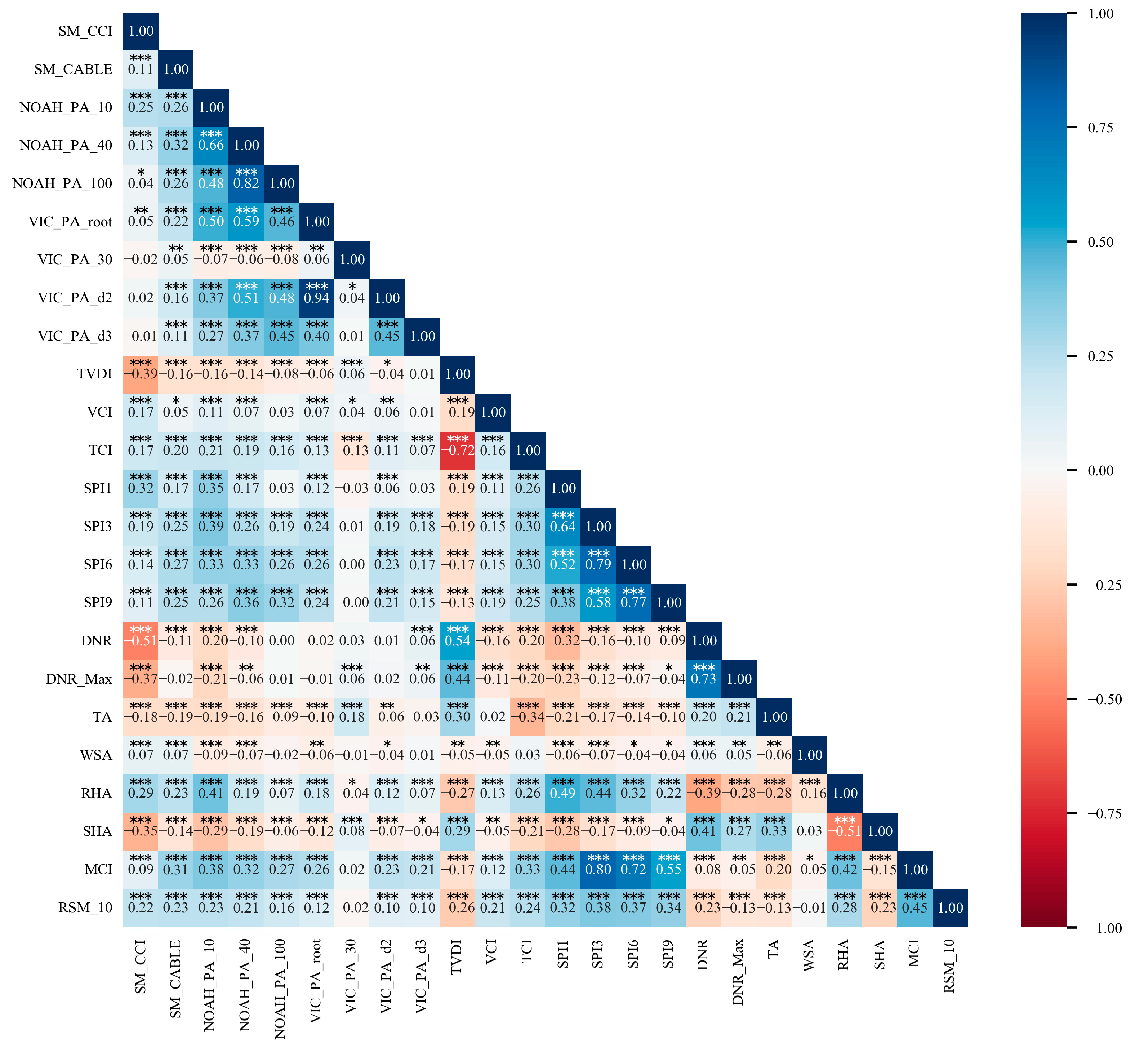
Figure 2 shows a heat map of the correlation coefficients between various drought indexes and RSM at a depth of 10 cm. It shows that there is strong collinearity between MCI, SPI3, and SPI6, and there is also strong collinearity between soil moisture anomalies at different depths in the GLDAS NOAH and VIC modes. Indexes, except for WSA and VIC_PA_30, are significantly correlated with RSM. The meteorological index, especially the MCI index, has a better correlation with RSM, but its correlation coefficient R is 0.45, and the determination coefficient R2 is about 0.2. In the meteorological index, RHA and SHA also show significant positive and negative correlation with RSM, followed by the correlation between optical remote sensing indexes and RSM. The correlation between the land surface model drought index and RSM is relatively the worst. It is obvious that it is difficult for a single index to accurately describe the temporal and spatial distribution characteristics of RSM. To simplify the model, collinear variables with poor correlation with RSM at different depths were removed.

3.1.2. Selection of Algorithm

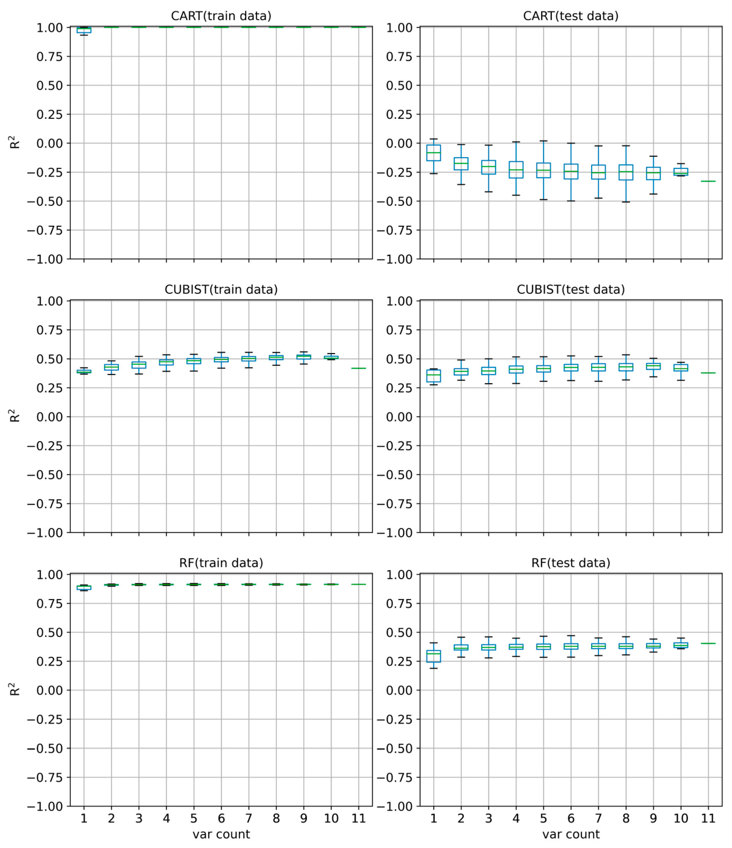
In the study, CART, Cubist and random forest (RF) algorithms, which were based on CARTs, were compared by using different numbers of input variables. R2 of these three algorithms on the training and test datasets is shown in Figure 3. It shows that although the R2 of the CART model in the training set is close to 1, the R2 on the test set is negative, indicating that the CART model performs very poorly on the test set and is severely overfitting. Although RF has significantly improved on the test set compared to CARTs, but RF is also significantly overfitting. Whereas the Cubist algorithm has similar R2 on the training and testing sets, it still performs well on the testing set and is better than RF. Therefore, the Cubist algorithm was chosen for estimating the soil moisture.

3.1.3. Selection of Environmental Factors

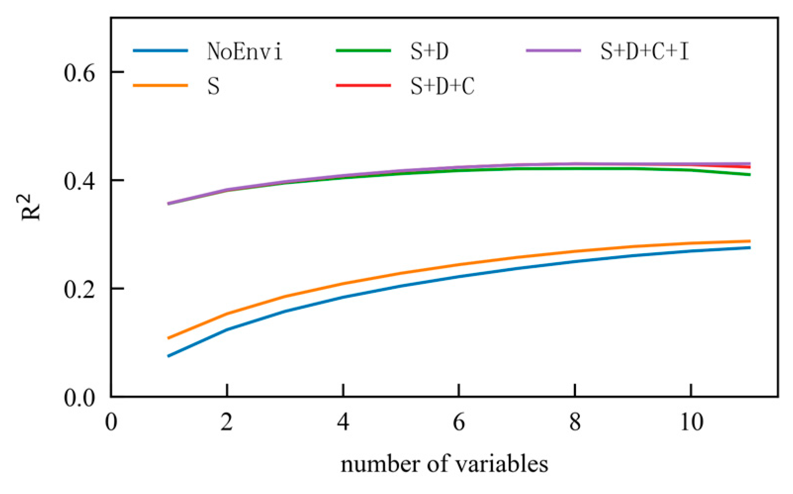
In the study, environmental factors such as season, DEM, climate zone, and irrigation type were considered. Taking a depth of 10 cm as an example, Figure 4 shows the R2 for cross validation of models considering different environmental factors. It shows that without considering any environmental factors, the R2 of the model on the test set increased with the number of variables, but the highest did not exceed 0.3, and the model performance was low. After adding season factors, the model performance was improved, but the improvement was not significant. After adding the DEM factor to the model, the performance of the model was significantly improved, and the impact of the number of variables on the model performance decreased. After adding the climate zoning factor to the model, the performance slightly improved. After adding the irrigation zoning factor, the model performance no longer increased. In addition, the accuracy of the comprehensive model increased slowly with an increase in the number of variables. After the number of variables exceeded 6, the accuracy of the model no longer increased. Overall, season, DEM, and climate zone environmental factors can improve model performance, especially the DEM factor. The results for depths of 20 cm and 50 cm are similar. Therefore, when constructing a comprehensive model, environmental factors such as season, DEM, and climate zone will be considered.

3.1.4. Selection of Variables

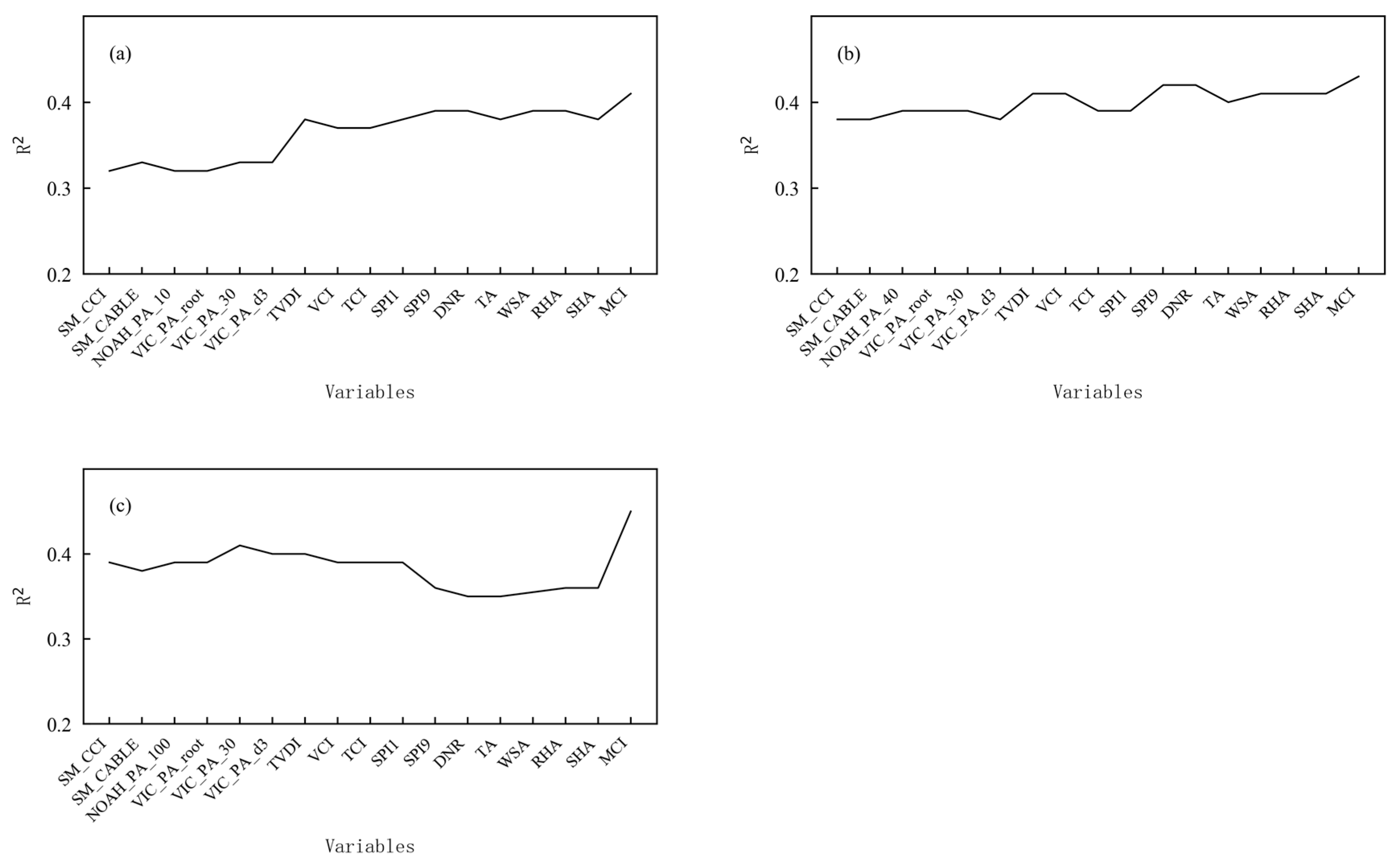
After adding variables one by one from the set of variables that removed collinear variables, a 5-fold cross validation was performed. The results are shown in Figure 5. It shows that TVDI and MCI can significantly improve the accuracy of the comprehensive model. SM_CABLE, SPI1, SPI9, WSA, and SHA can also improve the accuracy of the comprehensive model to a certain extent, so variables that are conducive to improving the accuracy of the model are selected to construct a comprehensive drought monitoring model (shown in Table 2).

3.2. Evaluation of the Comprehensive Model

3.2.1. Comprehensive Evaluation

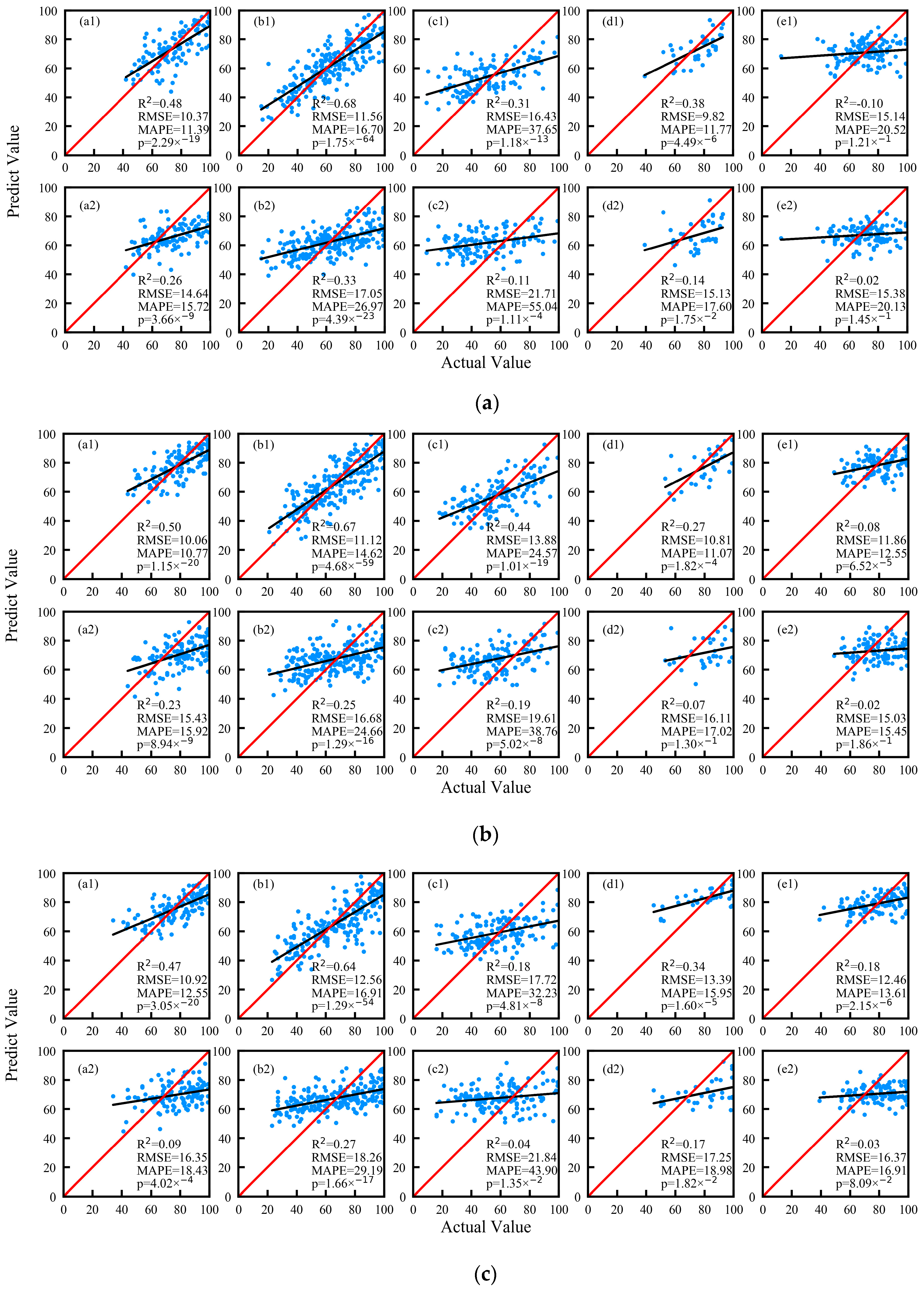
Based on the previous analysis, considering three environmental factors: season, DEM, and climate zone, a comprehensive agricultural drought monitoring model (hereinafter referred to as the comprehensive model) based on the Cubist algorithm was constructed using the variables shown in Table 1. Eighty percent of the data was used for modeling, 20% for validation and evaluation, and a single-variable model was also constructed. The modeling and validation accuracy of comprehensive models at different depths are shown in Table 3. Figure 6 shows the scatter plots of observed and fitted values of the validation data for comprehensive models and the MCI model with the best correlation at the 10 cm, 20 cm, and 50 cm depths. It shows that the three comprehensive models all have a certain degree of overfitting. There is a phenomenon that high values are underestimated and low values are overestimated. The accuracy of the comprehensive models is significantly improved compared with the single MCI model. RMSE and MAPE of the 10 cm, 20 cm, and 50 cm depth comprehensive models have an average decrease of about 26% and 28%, respectively, compared with the MCI model. Comparing the R2, RMSE, and MAPE of comprehensive models in different climate zones, it was found that the fitting results were significantly better in semi-humid areas, humid areas, and semi-arid areas. The shallow comprehensive model at a depth of 20 cm has the best fitting results in different climate zones, with a MAPE of about 11%~25% for each climate zone, followed by the comprehensive model at a depth of 10 cm, whose MAPE of each climate zone is about 12%~38%, and the comprehensive model at a depth of 50 cm, whose MAPE of each climate zone is about 13%~32%. At the same time, it is noted that the RSM in arid areas is mostly above 60%. Due to the low natural precipitation in arid areas, agricultural production uses irrigation, and the fitting of MCI models in arid areas is also poor. Irrigation may be an important reason for the relatively poor fitting of the comprehensive model and MCI model in this area.
Figure 7 shows the time series diagrams of actual and fitted values for several typical stations in different climate zones at a depth of 10 cm. It shows that the comprehensive model can simulate the variation characteristics of typical stations over time. The MAEP of actual and fitted values for stations in Gaotai, Minle, Yuzhong, Lintao, and Lixian are 10.8%, 8.8%, 19.4, 15.8%, and 12.6%, respectively. The actual RSM of Lixian, Lintao, and Yuzhong, located in humid, semi-humid, and semi-arid areas, fluctuates around 60%. Among them, Lixian and Lintao have more accurate simulations of high values, while Yuzhong has a lower simulation of high values and a heavier simulation of drought conditions. For example, after 2010, the actual RSM of Yuzhong was mostly above 60%, while the simulated RSM was lower than the actual one, reaching the level of light drought. The three stations have higher simulations of low values and a lighter simulation of drought conditions, such as in Lintao from 2009 to 2012, where the actual RSM was mostly below 60%; even below 40%, it reached the level of severe drought, while the simulated RSM was relatively high, only reaching the level of light to moderate drought. The actual RSM of Minle, located in semi-arid and semi-humid areas, and the Gaotai, located in arid areas, fluctuates around 80%, and the actual RSM also fluctuates around 80%, which is consistent with the actual situation without drought. The actual RSM of Minle has shown a downward trend since 2011, and the comprehensive model has simulated this change feature. The Gaotai fluctuates significantly around 80%, while the fluctuation simulated by the comprehensive model is slightly smaller.

3.2.2. Evaluation of the Impact of Environmental Factors on the Model

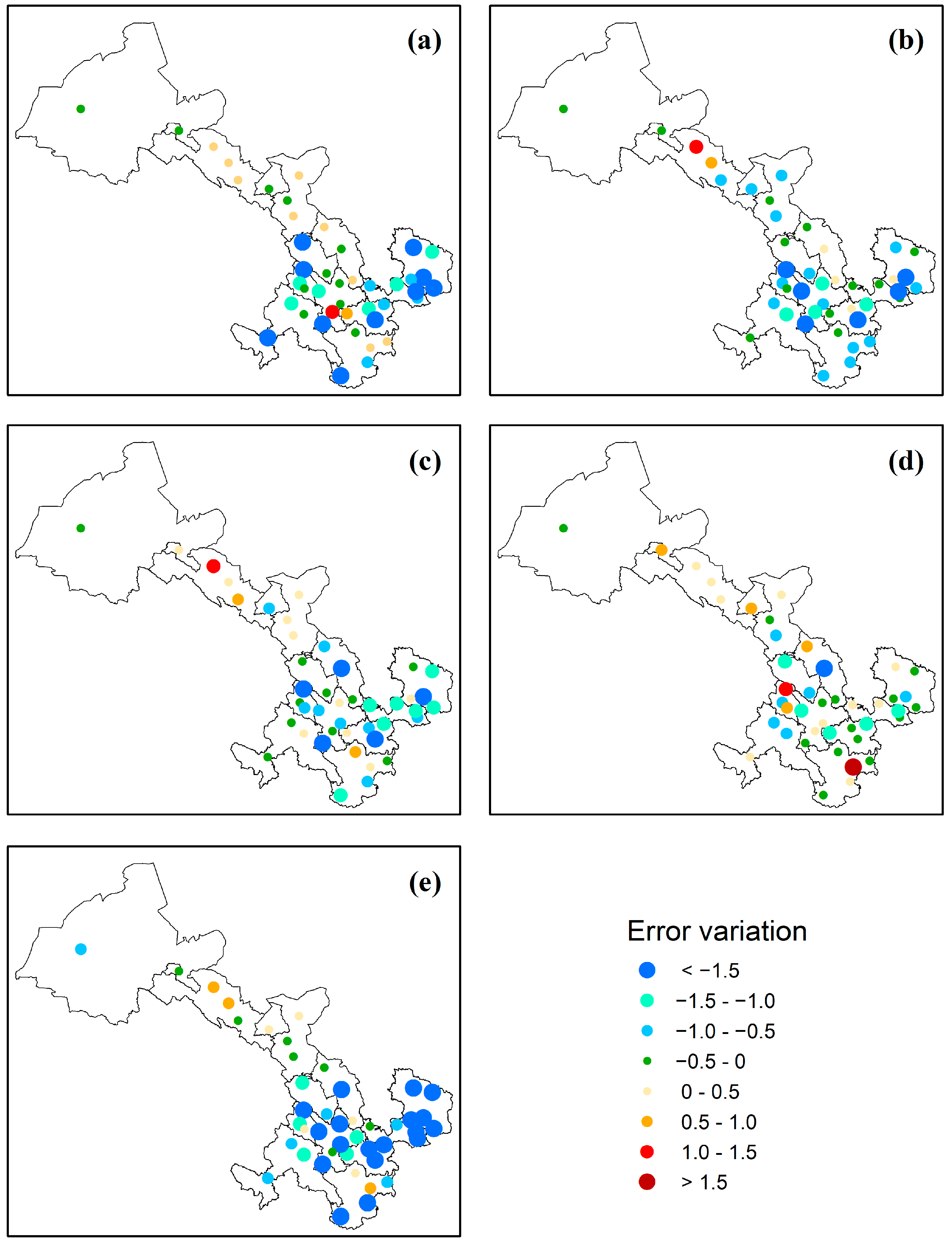
The RSME difference between the model without considering environmental factors and the model considering environmental factors for each station at 10 cm depth was calculated, and the spatial distribution is shown in Figure 8. After considering season, DEM, and climate zone, the errors of most stations decreased, and the model accuracy was greatly improved. Among them, the model’s accuracy was significantly improved after considering DEM factors. The station-averaged error difference at three depths is shown in Table 4. It shows that DEM, climate zone, and season factor alone can averagely reduce the error of the comprehensive model at three depths by about 20%, 7.5%, and 2.5%, respectively, and all three factors can averagely reduce the error by about 25%. This indicates that environmental factors, especially the DEM factor, are very crucial for establishing a comprehensive model based on the Cubist algorithm, even much more than increasing the number of input variables.
In order to understand the reasons why DEM can drastically improve accuracy in the comprehensive model, the following experiments were conducted. Using DEM and the variables in Table 2, the comprehensive model was constructed using the multiple regression algorithm and Cubist algorithm, respectively. The results of the training and testing sets are shown in Table 5. It shows that the fitting result of the multiple regression algorithm is significantly inferior to that of the Cubist algorithm. The core idea of the Cubist algorithm is to generate several multiple regression equations under the classification of rules. The multiple regression algorithm uses a single multiple regression equation throughout the entire research area. From the fitting results of both, the generation of rules in the Cubist algorithm is an important reason for the improvement of the comprehensive model accuracy of the Cubist algorithm. Table 6 shows the importance of each variable in the Cubist algorithm-based comprehensive model at 10 cm depth in both rules and models. It shows that DEM ranks first in terms of importance in rules, indicating that DEM is a very important classification indicator. It is the impact of DEM on rule generation that significantly improves the accuracy of the comprehensive model.

3.2.3. Evaluation of the Impact of Meteorological Factors on Comprehensive Models

The RSME difference between the model without considering the meteorological factors and the model considering the meteorological factors for each station was also calculated, and spatial distribution at 10 cm depth is shown in Figure 9. It shows that after considering MCI, SPI1, SPI9, and WSA, the error of most stations had decreased, while the error of some stations had increased. The stations with increased error are mostly distributed in the Hexi area, which is an arid area. Comparing Figure 8a–c, it is found that after considering SPI1, the errors of almost all stations had decreased to varying degrees, indicating that the precipitation in the past month was more conducive to reducing the error of the comprehensive model. The station-averaged error difference at three depths is shown in Table 7. Meteorological factors mainly reduce the error of shallow, comprehensive models. MCI, SPI1, SPI9, WSA, and SHA alone can averagely reduce the error of the comprehensive model at three depths by about 6.4%, 5.6%, 3.5%, 0.9%, and 1%, respectively. The comprehensive consideration of all five meteorological indexes can reduce the error at three depths by about 10.6%, 2.9%, and 5.9%, respectively. Overall, precipitation is still the most important meteorological factor affecting the accuracy of the comprehensive models, and WSA and SHA can slightly improve the accuracy of the comprehensive models at 10 cm and 20 cm.

3.3. Application of the Comprehensive Model

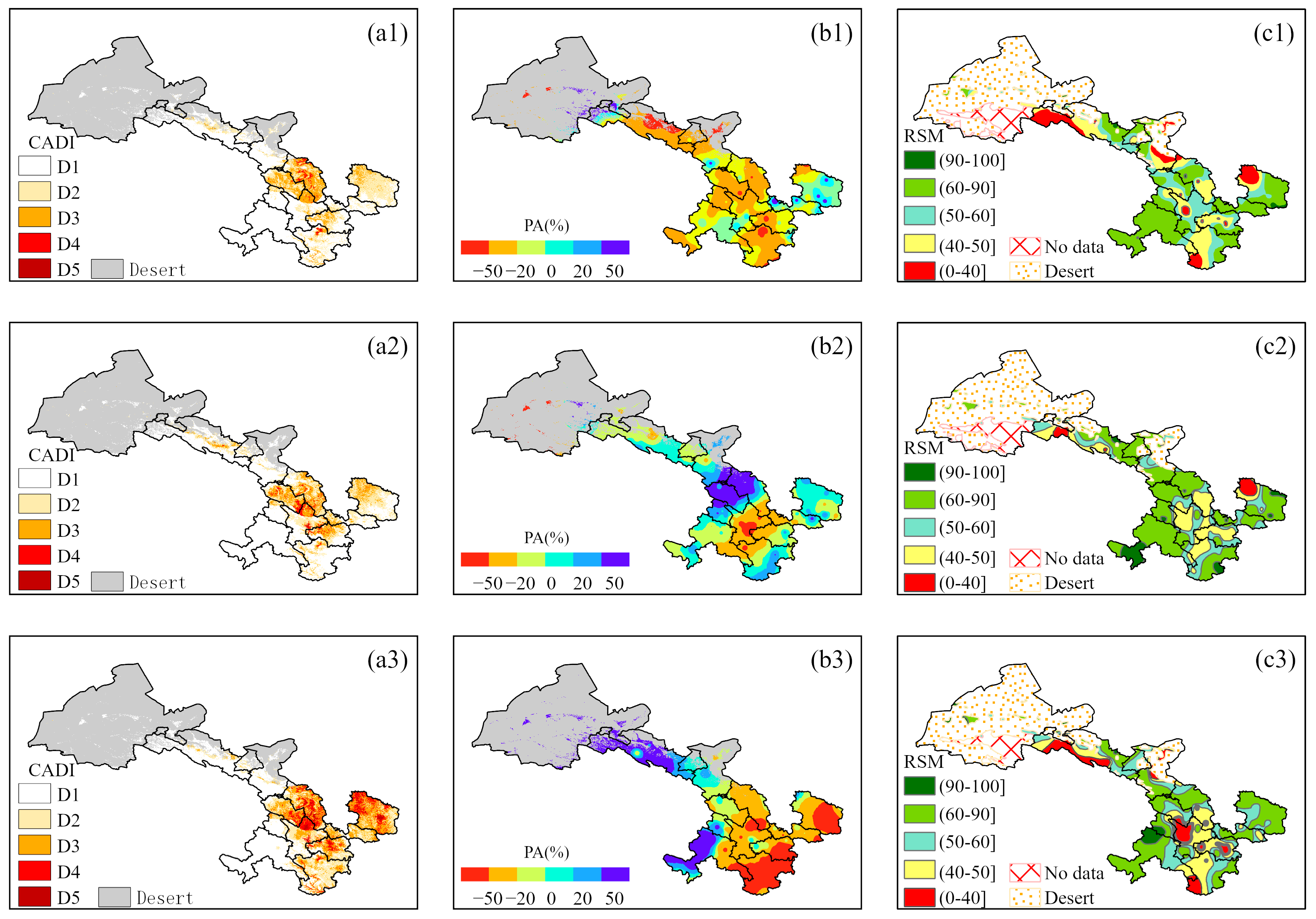
Since late July 2016, the average temperature in the central and eastern parts of Gansu Province has been around 2 °C higher, with the highest average temperature in nearly 56 years and the lowest precipitation in nearly 44 years. The high temperature and lack of precipitation have led to drought in the central and eastern parts of Gansu, with most of Dingxi city and the northwest of Tianshui city experiencing severe drought. Due to the lack of effective precipitation during the critical period of crops, local crops have suffered serious disasters, and potatoes and corn even have experienced widespread yield reductions or crop failures. Figure 10 shows the spatial distribution of the comprehensive drought index at 10 cm depth, percentage of precipitation anomaly, and actual RSM from June to August of 2016. It shows that after effective precipitation appeared in Lanzhou, Baiyin, northern Dingxi, and northern Qingyang in July, the drought situation in these areas was somewhat alleviated. However, by August, with the decrease in precipitation, the drought situation in these areas further intensified. Although the time scales, depths, and thresholds for drought classification are different, there is a certain degree of spatial consistency between drought classification classified by the comprehensive model and site RSM, which can indicate the spatial–temporal variation characteristics of this drought event in central Gansu province. Among them, CADI accurately reflects drought in northern Dingxi, Qingyang, Tianshui, and Longnan. However, CADI has a weak indication of drought in central Dingxi. There is a clear boundary phenomenon between semi-arid and semi-humid areas. The analysis for Figure 6 shows that the lower-fitting RSM of the typical semi-arid station and the higher-fitting RSM of the typical semi-humid station, especially the higher fitting in the semi-humid areas, are the reasons for the “boundary phenomenon” in this case.

4. Discussion

In the early study of soil moisture estimation models based on tree models, environmental factors were considered important factors regardless of the drought indexes considered. However, the importance of environmental factors in machine learning models was rarely discussed in previous research. This article attempts to reveal the importance of environmental factors in improving the accuracy of the Cubist algorithm, which provides a reference for a better understanding of the Cubist algorithm.
The core idea of the Cubist algorithm is to generate a series of rule-based regression equations, and environmental factors are important references for establishing rules. Establishing rules is actually an automatic division of regions in space, thereby achieving the automatic selection of indexes in regression equations. The large east–west span, large DEM span, and complex terrain in Gansu Province are important reasons for the underlying surface and complex climate. DEM is also the most important environmental factor affecting the accuracy of the comprehensive model. This indicates that selecting appropriate environmental factors for the study area using the Cubist algorithm is crucial for improving the model’s fitting ability.
However, the fitting accuracy of the integrated model is poor in the arid areas of Hexi and the semi-arid areas in the central region. On the one hand, although the average annual precipitation in the Hexi region is relatively low, the water resources provided by the Qilian Mountains can meet the irrigation needs of agriculture in the Hexi region. The lack of irrigation data may be an important reason for the low fitting accuracy of the comprehensive model of the Hexi arid area. In addition, SPI1 is the only meteorological factor that can improve the accuracy of the model in the Hexi region (Figure 9b), indicating that short-term precipitation has a more important impact on SM in the region. SPI1, which represents short-term precipitation, and MCI and SPI9, which represent long-term precipitation, have a positive effect on improving model accuracy in the Hedong region. Due to its arid climate characteristics, the soil sand content in the Hexi arid region is relatively high, while the soil clay content in humid and semi-humid areas is relatively high. The difference in soil properties may be an important factor in the different patterns of precipitation’s impact on SM in different regions. However, due to the high sand content, large rock and soil voids, and high groundwater level in the Hexi region, the ET0 (1049.3–1269.9 mm) is much higher than the precipitation (42–200 mm) [40]. Moreover, Zhang et al.’s [41] research shows that there is a strongly coupled nonlinear relationship between typical stations’ SM and evapotranspiration (EF) located in semi-arid areas. It can be seen that soil properties and evaporation are important factors affecting water cycling. The lack of soil properties and evaporation data may be another important reason for the low fitting accuracy in these regions.
At the same time, it is noted that the comprehensive model based on the Cubist algorithm exhibits obvious “boundary phenomena” in different climate zones, especially in semi-arid and semi-humid areas (Figure 10). The study uses the Cubist algorithm to achieve regression estimation of continuous soil moisture values, and divides soil moisture into drought levels with intervals of 10. Therefore, small errors may cause differences in drought levels. Low fitting accuracy in semi-arid areas is the important reason for the “boundary phenomena”. Apparently, the “boundary” is consistent with the climate zone. Although the consideration of climate zones can help improve the accuracy of comprehensive models, “boundary phenomena” also exist due to climate zones.

5. Conclusions

(1)
Among the comprehensive models constructed by the Cubist algorithm, the model at 20 cm depth has the highest accuracy, followed by the models at 10 cm and 50 cm depths. The validation R2 of the comprehensive model at 10 cm, 20 cm, and 50 cm depth is 0.56, 0.57, and 0.54, and the RMSE is 13.1, 12.8, and 13.2, respectively. The MAPEs are about 20.3%, 18.6%, and 18.6%, respectively. The accuracy of the comprehensive model has been significantly improved compared to the single-variable model. The RMSE and MAPE of the comprehensive model has decreased by about 26% and 28% compared to the best MCI model, on average, at the 10 cm, 20 cm, and 50 cm depths.
(2)
The fitting accuracy of the comprehensive model in humid areas and semi-humid areas, as well as semi-arid and semi-humid areas, is significantly higher than that in arid and semi-arid areas. In humid areas, semi-humid areas, semi-arid and semi-humid areas, semi-arid areas, and arid areas, the average validation R2 of the comprehensive model at 10 cm, 20 cm, and 50 cm depth is 0.48, 0.66, 0.31, 0.33, and 0.16, respectively. The average RMSE is 10.5, 11.7, 16, 11.3, and 13.2, and MAPEs are about 11.6%, 16.1%, 31.5%, 12.9%, and 16.5%, respectively.
(3)
Environmental factors play a crucial role in improving the accuracy of comprehensive models, with a greater impact than increasing the number of drought indicators. Considering that the DEM, climate zone, season alone can averagely reduce the error by about 20%, 7.5%, and 2.5%, respectively, and considering that all three factors can averagely reduce the error by about 25%. Compared to environmental factors, meteorological factors have a slightly weaker effect on improving the accuracy of comprehensive models. The consideration of meteorological factors, such as precipitation, WS, and SH, averagely reduce the error by about 6.5%.
(4)
The lack of irrigation, soil property, and evapotranspiration data, especially the lack of evapotranspiration data, may be an important reason for the low fitting accuracy of the comprehensive model in the arid and semi-arid areas of Hexi. In the future, efforts will be made to introduce water content information, such as irrigation, soil properties, and evapotranspiration data, into the comprehensive model, in order to improve the soil moisture-monitoring ability in the Hexi region.
(5)
Classification is another major task of machine learning algorithms, which can directly obtain drought levels and may improve the accuracy of drought levels. In the future, it will be necessary to compare the results of machine learning regression algorithms and classification algorithms to improve the accuracy of drought levels, especially in the division of drought levels in semi-arid and arid areas. In addition, the “boundary phenomenon” exists due to climate zone, and climate zone is based on multiple indicators, such as precipitation, dryness, temperature, and accumulated temperature [24]. Therefore, in addition to improving the fitting accuracy of regression models or the accuracy of classification models, using zoning indicators instead of climate zone may improve this situation. However, further research is needed to discover the impact of these factors on the comprehensive model.

Author Contributions

Conceptualization, S.S.; methodology, S.S. and L.W; software, L.W.; validation, D.H.; formal analysis, S.S.; investigation, X.W.; resources, L.Z.; writing—original draft preparation, S.S.; writing—review and editing, S.S and Y.R.; visualization, S.S. All authors have read and agreed to the published version of the manuscript.

Funding

This study was supported by the National Natural Science Foundation of China (Grant Nos. 42105131, 42075120, and 41875020), the Meteorological Science and Technology Research Project of Gansu Provincial Meteorological Bureau (ZcZd2022-26), and the Innovation Team of Lanzhou Institute of Arid Meteorology, CMA (GHACXTD-2020-4).

Data Availability Statement

Conflicts of Interest

The authors declare no conflict of interest.

References

  1. Guo, N.; Wang, X. Advances and Developing Opportunities in Remote Sensing of Drought. J. Arid. Meteorol. 2015, 33, 1–18. [Google Scholar]
  2. Liu, H.; Wang, F.; Zhang, T. Evaluation applicability of CLDAS and GLDAS soil moisture for the Loess Plateau. Agric. Res. Arid. Areas 2018, 36, 270–276. [Google Scholar]
  3. Kowalczyk, E.A.; Wang, Y.P.; Law, R.M.; Davies, H.L.; McGregor, J.L.; Abramowitz, G. CSIRO Atmosphere Biosphere Land Exchange Model for Use in Climate Models and as an Offline Model; CSIRO Marine and Atmospheric Technical Report; Commonwealth Scientific and Industrial Research Organisation: Canberra, Australia, 2006; pp. 1–37. [Google Scholar]
  4. Yang, X.; Yang, Q. Research on meteorological drought severity model for Loess Plateau in Gansu. J. Nat. Disasters 2007, 16, 30–36. [Google Scholar]
  5. Zhang, L.; Zhang, Q.; Zhang, H.; Yue, P.; Li, H.; Wang, J.; Zhao, F.; Wang, Y.; Wang, J. Environmental factors driving evapotranspiration over a grassland in a transitional climate zone in China. Meteorol. Appl. 2022, 29, e2066. [Google Scholar] [CrossRef]
  6. Zhang, Q.; Hu, Y.; Cao, X.; Liu, W. On Some Problems of Arid Climate System of Northwest China. J. Desert Res. 2000, 20, 357–362. [Google Scholar]
  7. Yang, S.; Liu, C. Remote sensing calculation of soil moisture and analysis of water cycle process in the Yellow River Basin. Sci. China Ser. E Technol. Sci. 2004, 34, 1–12. [Google Scholar] [CrossRef]
  8. Zhou, S.; Williams, A.; Lintner, B.; Berg, A.; Zhang, Y.; Keenan, T.; Cook, B.; Hagemann, S.; Seneviratne, S.; Gentine, P. Soil moisture–atmosphere feedbacks mitigate declining water availability in drylands. Nat. Clim. Chang. 2021, 11, 38–44. [Google Scholar] [CrossRef]
  9. Brown, J.; Wardlow, B.; Tadesse, T.; Hayes, M.; Reed, B. The Vegetation Drought Response Index (VegDRI): A New Integrated Approach for Monitoring Drought Stress in Vegetation. GISci. Remote Sens. 2008, 45, 16–46. [Google Scholar] [CrossRef]
  10. Sánchez, N.; González-Zamora, Á.; Piles, M.; Martínez-Fernández, J. A New Soil Moisture Agricultural Drought Index (SMADI) Integrating MODIS and SMOS Products: A Case of Study over the Iberian Peninsula. Remote Sens. 2016, 8, 287. [Google Scholar] [CrossRef]
  11. Sun, P.; Zhang, Q.; Wen, Q.; Singh, V.; Shi, P. Multisource data based integrated agricultural drought monitoring in the Huai River basin, China. J. Geophys. Res. Atmos. 2017, 122, 10751–10772. [Google Scholar] [CrossRef]
  12. Ji, T.; Li, G.; Yang, H.; Liu, R.; He, T. Comprehensive drought index as an indicator for use in drought monitoring integrating multi-source remote sensing data: A case study covering the Sichuan-Chongqing region. Int. J. Remote Sens. 2018, 39, 786–809. [Google Scholar] [CrossRef]
  13. Wang, J.; Zhu, X.; Liu, X.; Pan, Y. Research on agriculture drought monitoring method of Henan Province with multi-sources data. Remote Sens. Land Resour. 2018, 30, 180–186. [Google Scholar]
  14. Bijaber, N.; El Hadani, D.; Saidi, M.; Svoboda, M.D.; Wardlow, B.D.; Hain, C.R.; Poulsen, C.C.; Yessef, M.; Rochdi, A. Developing a Remotely Sensed Drought Monitoring Indicator for Morocco. Geosciences 2018, 8, 55. [Google Scholar] [CrossRef] [PubMed]
  15. Meng, L.; Dong, T.; Zhang, W. Drought monitoring using an Integrated Drought Condition Index (IDCI) derived from multi-sensor remote sensing data. Nat. Hazards 2016, 80, 1135–1152. [Google Scholar] [CrossRef]
  16. Zhang, X.; Chen, N.; Li, J.; Chen, Z. Multi-sensor integrated framework and index for agricultural drought monitoring. Remote Sens. Environ. 2017, 188, 141–163. [Google Scholar] [CrossRef]
  17. Peng, X.; Wang, Q.; Yuan, C.; Lin, K. Review of research on data mining in application of meteorological forecasting. J. Arid. Meteorol. 2015, 33, 19–27. [Google Scholar]
  18. Han, J.; Mao, K.; Xu, T.; Guo, J.; Zuo, Z.; Gao, C. A Soil Moisture Estimation Framework Based on the CART Algorithm and Its Application in China. J. Hydrol. 2018, 563, 65–75. [Google Scholar] [CrossRef]
  19. Yang, J.; Zhang, S.; Bai, Y.; Huang, A.; Zhang, J. SPEI Simulation for Monitoring Drought Based Machine Learning Integrating Multi-Source Remote Sensing Data in Shandong. Chin. J. Agrometeorol. 2021, 42, 230–242. [Google Scholar]
  20. Shen, R.; Huang, A.; Li, B.; Guo, J. Construction of a drought monitoring model using deep learning based on multi-source remote sensing data. Int. J. Appl. Earth Obs. Geoinf. 2019, 79, 48–57. [Google Scholar] [CrossRef]
  21. Breiman, L.; Friedman, J.; Olshen, R.; Stone, C.; Olshen, R. Classification and Regression Trees; Chapman and Hall: New York, NY, USA, 1984. [Google Scholar]
  22. Demisse, G.; Tadesse, T.; Bayissa, Y.; Atnatu, S.; Argaw, M.; Nedaw, D. Vegetation condition prediction for drought monitoring in pastoralist areas: A case study in Ethiopia. Int. J. Remote Sens. 2018, 39, 4599–4615. [Google Scholar] [CrossRef]
  23. Nam, H.; Tadesse, T.; Wardlow, B.; Hayes, M.; Svoboda, M.; Hong, E.; Pachepsky, Y.; Jang, M. Developing the vegetation drought response index for South Korea (VegDRI-SKorea) to assess the vegetation condition during drought events. Int. J. Remote Sens. 2018, 39, 1548–1574. [Google Scholar] [CrossRef]
  24. Bao, W. Gansu Climate; China Meteorological Press: Beijing, China, 2018; 283p. [Google Scholar]
  25. Deng, Z.; Xie, J.; Liu, X.; Yin, D. The Characteristics and Development and Utilization of Climate Resources in Gansu Province. J. Arid. Meteorol. 1998, 16, 16–19. [Google Scholar]
  26. GB/T20481-2006; Classification of Meteorological Drought. National Climate Center: Beijing, China, 2006; pp. 1–17.
  27. Kogan, F. Remote sensing of weather impacts on vegetation in non-homogeneous areas. Int. J. Remote Sens. 1990, 11, 1405–1419. [Google Scholar] [CrossRef]
  28. Kogan, F. Application of vegetation index and brightness temperature for drought detection. Adv. Space Res. 1995, 15, 91–100. [Google Scholar] [CrossRef]
  29. Sandholt, I.; Rasmussen, K.; Andersen, J. A simple interpretation of the surface temperature—Vegetation index space for assessment of surface moisture status. Remote Sens. Environ. 2002, 79, 213–224. [Google Scholar] [CrossRef]
  30. Mcnally, A.; Shukla, S.; Arsenault, K.; Wang, S.; Peters-Lidard, C.D.; Verdin, J.P. Evaluating ESA CCI soil moisture in East Africa. Int. J. Appl. Earth Obs. Geoinf. 2016, 48, 96–109. [Google Scholar] [CrossRef] [PubMed]
  31. Shen, X.; An, R.; Quaye-Ballard, J.; Zhang, L.; Wang, Z. Evaluation of the European Space Agency Climate Change Initiative Soil Moisture Product over China Using Variance Reduction Factor. J. Am. Water Resour. Assoc. 2016, 52, 1524–1535. [Google Scholar] [CrossRef]
  32. Xu, W. Educational Statistics, 2nd ed.; Nanjing Normal University Press: Nanjing, China, 2007. [Google Scholar]
  33. Li, Y.; Zhang, L.; Zhang, H.; Pu, X. Drought Monitoring Based on CABLE Land Surface Model and Its Effect Examination of Typical Drought Events. Plateau Meteorol. 2015, 34, 1005–1018. (In Chinese) [Google Scholar] [CrossRef]
  34. Zhang, L. Drought Monitoring Technique Based on Land Surface Model and the Study of its Application Effects in China. Ph.D. Thesis, Lanzhou University, Lanzhou, China, 2016. [Google Scholar]
  35. Deng, H.; Lu, Y.; Wang, Y.; Chen, X.; Liu, Q. Assessment of Actual Evapotranspiration in the Minjiang River Basin Based on the GLDAS-Noah Model. Sci. Geogr. Sin. 2022, 42, 548–556. [Google Scholar]
  36. Liu, P.; Song, H.; Bao, W.; Li, J. Applicability Evaluation of CLDAS and GLDAS Soil Temperature Data in Shaanxi Province. Meteorol. Sci. Technol. 2021, 49, 604–611. [Google Scholar]
  37. Breiman, L. Random Forests. Machine Learning. 2001, 45, 5–32. [Google Scholar] [CrossRef]
  38. Quinlan, J. C4.5: Programs for Machine Learning; Morgan Kaufmann Publishers Inc.: San Francisco, CA, USA, 1993. [Google Scholar]
  39. Data Mining with Cubist. Available online: http://www.rulequest.com/cubist-info.html (accessed on 4 April 2022).
  40. Ma, Y.; Sun, D.; Zhang, R.; Xu, J.; Wang, X. Analysis of driving factors for spatiotemporal variation of reference crop evapotranspiration in Gansu Province. Chin. Agric. Meteorol. 2022, 43, 881–892. [Google Scholar]
  41. Zhang, L.; Sha, S.; Zhang, Q.; Zhao, F.; Zhao, J.; Li, H.; Wang, S.; Wang, J.; Hu, Y.; Han, H. Investigating the Coupling Relationship between Soil Moisture and Evaporative Fraction over China’s Transitional Climate Zone. Hydrology 2023, 10, 221. [Google Scholar] [CrossRef]
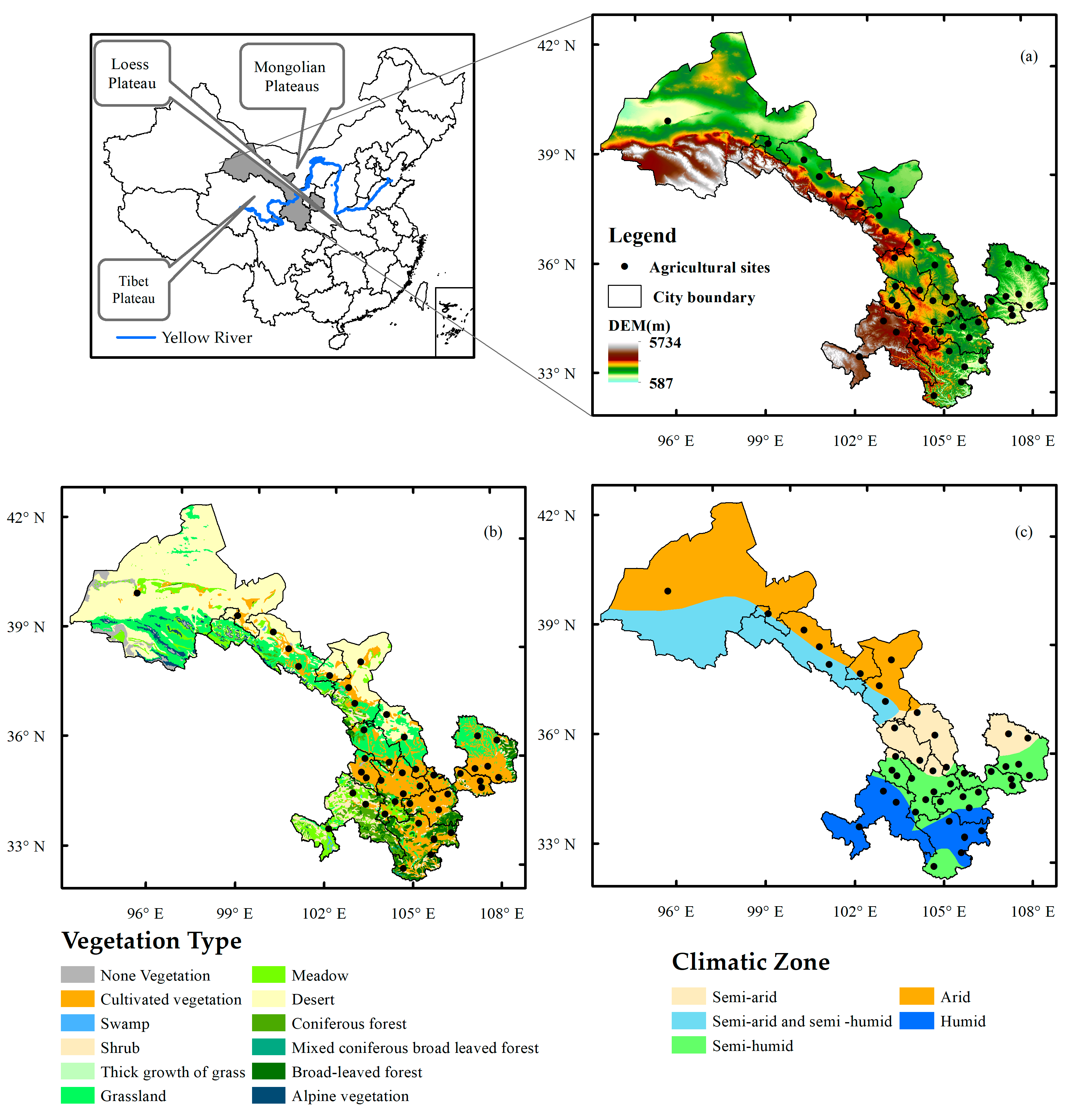
Figure 1. Geographical location (a), vegetation type (b), and climate zone diagram of Gansu Province (c).
Hydrology 11 00100 g001
Figure 2. Heat map of the correlation between drought indexes and RSM at a depth of 10 cm. In the figure, * represents p < 0.05, ** represents p < 0.01, *** represents p < 0.001.
Hydrology 11 00100 g002
Figure 3. The box diagram of R2 of CART, Cubist, and RF in training and test data sets by using different numbers of input variables.
Hydrology 11 00100 g003
Figure 4. Cross-validation results of model accuracy under different environmental factors at a depth of 10 cm (In the figure, “NoEnvi” represents no environmental factors, while “S”, “D”, “C”, “I” represent season, DEM, climate zone, and irrigation, respectively).
Hydrology 11 00100 g004
Figure 5. Cross-validation results after adding different variables to the variable sets at 10 cm depth (a), 20 cm depth (b), and 50 cm depth (c).
Hydrology 11 00100 g005
Figure 6. Scatter plots of observation and fitting values for the comprehensive model and MCI model at depths of 10 cm (a), 20 cm (b), and 50 cm (c) on the test dataset (In the figure, (a)~(e) represent humid areas, semi-humid areas, semi-arid areas, semi-arid and semi-humid areas, and arid areas, respectively; 1 and 2 represent the comprehensive model and MCI model, respectively).
Hydrology 11 00100 g006
Figure 7. Time series diagrams of the true and predicted RSM at a depth of 10 cm depth at Gaotai (a), Minle (b), Yuzhong (c), Lintao (d), and Lixian (e) in different climate zones (Gaotai, Minle, Yuzhong, Lintao, and Lixian are located in arid areas, semi-arid and semi-humid areas, semi-arid areas, semi-humid areas, and humid areas, respectively).
Hydrology 11 00100 g007
Figure 8. Spatial distribution diagram of the RSME difference between the model without considering environmental factors and the model considering environmental factors ((a) is only considering season factors, (b) is only considering DEM factors, (c) is only considering climate zone factors, and (d) is considering all three factors simultaneously).
Hydrology 11 00100 g008
Figure 9. Spatial distribution diagram of the RSME difference between the model without considering meteorological factors and the model considering meteorological factors at 10 cm depth ((a) is only considering MCI, (b) is only considering SPI1, (c) is only considering SPI9, (d) is only considering WSA, (e) is considering MCI, SPI1, SPI9, and WSA simultaneously).
Hydrology 11 00100 g009
Figure 10. The drought classification map of the comprehensive agricultural drought index at 10 cm depth in June (a1), July (a2), and August (a3) of 2016, and the percentage of precipitation anomalies in June (b1), July (b2), and August (b3), as well as the actual RSM at 0–30 cm depth on June 16 (c1), July 16 (c2), and August 16 (c3).
Hydrology 11 00100 g010
Table 1. Drought classification based on RSM.
Agricultural Drought GradeClassification
None drought D160% < RSM
Light drought D250% < RSM ≤ 60%
Moderate drought D340% < RSM ≤ 50%
Severe drought D430% < RSM ≤ 40%
Extreme drought D5RSM ≤ 30%
Table 2. Variables used to build the comprehensive drought monitoring model.
DepthVariables
10 cmMCI, TVDI, SPI1, SPI9, SM_CABLE, WSA
20 cmNOAH_10_40 cm_PA, TVDI, SPI9, WSA, SHA, MCI
50 cmNOAH_40_100 cm_PA, VIC_PA_30, MCI
Table 3. Comprehensive model accuracy evaluation.
Depth Training Data Set Test Data Set
Sample SizeR2p-ValueRMSEMAPESample SizeR2p-ValueRMSEMAPE
10 cm26360.71 010.19 15.24 6590.56 2.19 × 10−11813.10 20.33
20 cm26210.75 09.44 12.72 6560.57 1.88 × 10−12412.77 18.57
50 cm26870.67 011.31 15.81 6720.54 1.07 × 10−11613.23 18.62
Table 4. Statistical table for the station-averaged RMSE difference, considering different environmental factors.
DepthError Variation
of Season
Error Variation
of DEM
Error Variation
of Climate Zone
Error Variation
of Three Factors
Absolute ValueRelative ValueAbsolute ValueRelative ValueAbsolute ValueRelative ValueAbsolute ValueRelative Value
10 cm−0.4−3%−2.4−14.3−1−5.7%−3.2−22%
20 cm−0.4−3%−2.8−18%−1.2−7.6%−3.7−26%
50 cm−0.2−1.3%−3.2−20%−1.59%−4.2−26%
Table 5. The fitting results of multiple regression algorithm and Cubist algorithm.
AlgorithmDepthTraining Data Set Test Data Set
R2RMSEMAPER2RMSEMAPE
multiple regression10 cm0.27 16.24 25.73 0.28 16.74 27.64
20 cm0.26 16.15 23.04 0.25 16.93 26.16
50 cm0.17 17.86 27.22 0.15 18.06 26.89
Cubist10 cm0.65 11.28 17.240.47 14.29 22.94
20 cm0.68 10.61 14.250.50 13.85 20.15
50 cm0.57 12.79 18.180.45 14.55 21
Table 6. The importance of various variables in the 10 cm Cubist algorithm integrated model in rules and models.
VariablesRulesModels
DEM8687
MCI4193
TVDI1282
SPI1668
SPI9459
SM_CABLE245
WSA129
Table 7. Statistics of mean station error for models considering different meteorological factors.
DepthMCI SPI1 SPI9 WS SHConsidering All
ar (%)ar(%)ar (%)ar (%)ar(%)ar (%)
10 cm−0.8−6.7−0.7−5.6−0.5−4.1−0.2−1.48--−1.27−10.6
20 cm−0.7−6.5--−0.3−2.8−0.01−0.25−0.13−1−0.51−2.9
50 cm−0.7−5.9--------−0.7−5.9
Note: In the table, a and r represent absolute and relative values, respectively, and “-” indicates that this factor has not been considered.
Disclaimer/Publisher’s Note: The statements, opinions and data contained in all publications are solely those of the individual author(s) and contributor(s) and not of MDPI and/or the editor(s). MDPI and/or the editor(s) disclaim responsibility for any injury to people or property resulting from any ideas, methods, instructions or products referred to in the content.