Article

Characterizing Soil and Bedrock Water Use of Native California Vegetation

1
Earth Knowledge, Inc., Davis, CA 95616, USA
2
U.S. Geological Survey California Water Science Center, Sacramento, CA 95819, USA
3
Department of Environmental Science and Policy, University of California, Davis, CA 95616, USA
4
School of Natural Resources, University of California, Berkeley, CA 94720, USA
*
Author to whom correspondence should be addressed.
Hydrology 2024, 11(12), 211; https://doi.org/10.3390/hydrology11120211
Submission received: 5 November 2024 / Revised: 29 November 2024 / Accepted: 1 December 2024 / Published: 8 December 2024
(This article belongs to the Section Hydrological and Hydrodynamic Processes and Modelling)

Abstract

:
The effective characterization of landscape water balance components—evapotranspiration, runoff, recharge, and soil storage—is critical for understanding the integrated effects of the water balance on vegetation dynamics, water availability, and associated environmental responses to climate change. An improved parameterization of these components can improve assessments of landscape stress and provide useful insights for predicting and managing vegetation responses to climate change. Hydrology models typically are not able to address water availability below the mapped soil profile, but we refined a landscape hydrology model, the Basin Characterization Model, by balancing measures of actual evapotranspiration (AET) with modeled subsurface soil water holding capacity, including bedrock storage. The purpose of this study was to characterize the effective rooting depth (the depth of soil and bedrock storage required to support AET) for 35 native vegetation types in California in order to quantify soil and bedrock water use, which ranged from 0 to 3.1 m for most vegetation types, exceeding mapped soil depths. This resulted in the quantification of bedrock water use, increasing available water 67% over that calculated by mapped soils alone. We found that mid-elevation vegetation types with lower water and energy limitations have the highest evapotranspiration rates and deepest effective rooting depth. We also evaluated the resilience to drought with this more spatially realistic characterization of water and vegetation interactions.

1. Introduction

The degree to which a terrestrial site can mediate impacts of climate change depends on its vegetation type, energy balance and climate, and on available water for actual evapotranspiration (AET) to support plant growth. Available water depends in part on the depth of the soil, and underlying bedrock, which can buffer drying conditions with the soil moisture it contains that is available to plants [1]. Recent droughts in California provide examples of soils drying past the wilting point [2], and how substantial rainfall following drought conditions did not result in runoff because the precipitation was filling up the unsaturated zone or subsurface bedrock [3,4,5]. Particularly for locations with seasonally decoupled water and energy, such as Mediterranean-type climates in which rain falls in winter, the quantification of the water balance for landscapes and watersheds is critical to understanding how resilient they may be to droughts or forest die-off, to ameliorating projected increases in peak runoff events, or simply to understanding how best to manage natural resources for watershed health and water supply.
In California, 85% of surface water supply comes from forested headwater basins with an annual snowpack, primarily in the Sierra Nevada. In recent years, climatic stresses on these forests have also contributed to extreme wildfires [6] and tree mortality [7], exacerbating water quality concerns [8,9]. This is in line with projections that climatic water demand in these forests will intensify, even under future climates that have higher precipitation, due to rapidly increasing air temperatures [10]. The trend of intensifying forest stress may follow elevational gradients [11], such as those that Goulden and Bales [12] describe, with a projected increase in AET in the Sierra Nevada as vegetation with higher AET moves upslope as cold weather limitations are relaxed. It is increasingly important to be able to accurately characterize the water balance and the contributions of different vegetation types to total AET in these watersheds.
Research in recent years has demonstrated that woody plants use substantial volumes of water from bedrock to support their AET [1,13]. The water storage capacity of bedrock can explain ecosystem distributions and drought vulnerability [14,15,16], and as climate change increases it becomes increasingly important to quantify this storage capacity in order to predict large-scale vegetation dynamics and water supply, including the stability or vulnerability of ecosystem carbon storage [1]. Hydrologic models do not specifically or mechanistically incorporate bedrock storage capacity in their characterization of the water balance and subsequent hydrologic and energy partitioning.
In addition to topo-climatic drivers, accurate estimates of plant available water storage rely on an understanding of the depth to which the roots of vegetation may extend to access available water. Native vegetation does not transpire at the rate of potential evapotranspiration (PET) but is limited to less than the potential by physiological traits of the vegetation and by the soil/bedrock moisture availability in the root zone [17]. Limitations to full PET may also vary seasonally for different vegetation types and for different climates, even if sufficient water is available. Historical methods developed to conceptualize these limits do not differentiate among native vegetation species and under different climatic conditions. These limits, represented as a reduction below PET, have been used for decades in agriculture as transpiration coefficients for assessing irrigation needs [18,19]. The core of these methods is the determination of the crop transpiration coefficient (Kc), which represents the AET of a given crop as a proportion of the PET of an ideal (reference) crop grown under no limitations of water and nutrients. There are serious limitations when assumed Kc values are not correct [20], leading to on-going efforts to further refine models of plant-environmental processes. Mata-Gonzalez et al. [21] did a review of methods as they are applied to the native vegetation of arid lands, which grow in conditions that clearly depart from those of irrigated crops. Allen et al. [19] proposed the use of adjustment factors to recalculate Kc in plants subject to water deficits. Wyatt et al. [22] used adjustment factors for four native vegetation types that deviated substantially from those at nearby grassland monitoring sites used for crop coefficients. Understanding the seasonal limits to AET for different vegetation types is imperative for calculating an accurate water balance across the landscape, quantifying AET, and assessing how these limits may change as precipitation or temperature patterns change.
Here, we address two difficulties in assessing the regional AET patterns of native vegetation for the purpose of assessing vulnerabilities to climate. One difficulty is to assess and quantify actual water storage available for plant AET, including soil storage and shallow bedrock storage, especially for forest lands. This was assessed for woody plants in the Mediterranean parts of the US by McCormick et al. [1] with a simple water balance calculation that used only precipitation, actual evapotranspiration estimates, and soil water holding capacity, without detailed energy balance calculations or species-specific AET. They found soil depth defined in the Natural Resources Conservation Service (NRCS) SSURGO or STATSGO soil maps does not capture the extent of plant rooting depth, and they calculated the water storage in bedrock by the extent of AET that exceeded precipitation for a given month. However, quantifying rooting depth and bedrock storage is difficult for large areas and varied vegetation types. There is a need to improve the estimates of soil depth explored by vegetation roots to more accurately model large-area water balance dynamics, particularly as the climate warms.
The metric that is most useful to such hydrologic studies is the total volume of subsurface materials that are explored by roots, what we call the effective rooting depth, which may incorporate penetration of roots into underlying bedrock material, but with different water use rates throughout the root zone. Klos et al. [23] highlight the importance of subsurface water storage in Sierra Nevada soils up to 10–20 m deep that are accessible to trees and sustain them through the dry season and extended droughts. Flint and Childs [24] characterized the capacity of rock fragments in skeletal soils to hold from 2 to 48% of the total available water in the soil profile. An approach was taken by Ichii et al. [25] to improve estimates of rooting depths in California using satellite based AET and an ecosystem model for plant functional types. The estimates of AET were constrained by eddy covariance measurements at several stations and inferred rooting depths by the length of sustained AET through the growing season. This approach did not include the quantification of the individual water balance components that may be differentially constrained across the landscape.
A second difficulty is the assessment of plant AET. Typical methods to measure it include remotely sensed data that are constrained by field observations of flux, and results vary widely among datasets. Although remote sensing methods excel at depicting spatial and temporal variability, the estimation of ET independently of other water budget components can lead to inconsistency with other budget terms [26]. An effort to quantify vegetation-specific ET linked to both soil and bedrock water requires an ET product developed using a water balance approach along with remote sensing products, and ground truthing flux measurements as employed by Reitz et al. [26].
In this paper, we present a unique approach to describing the response of 35 native vegetation types in California to climate and available water by characterizing an effective rooting depth, the storage required to supply observed AET, that explores reservoirs of water stored below the mapped soil depth in weathered, fractured, or permeable bedrock, along with a monthly coefficient describing seasonal limits of evapotranspiration. Here, we ask (1) can bedrock water use be quantified across the landscape specifically for varying vegetation types, including woody plants and non-woody perennial and annual vegetation and (2) can we illustrate potential buffers to climate change-driven vegetation stress on the basis of the additional water available in bedrock for transpiration? This study successfully quantifies bedrock water use through the novel characterization of an effective rooting depth. This serves to improve the water balance calculations that can inform evaluations of vegetation risk because of changes in climate as well as to improve estimates for water resource assessments and forecasts. We illustrate the efficacy of these improved characterizations on the spatially distributed response of the landscape to drought.

2. Materials and Methods

2.1. Overview

The approach to estimating soil depth, effective rooting depth, and quantifying AET use from soil and bedrock for each of 35 vegetation types relied on the application of a regional water balance model, the Basin Characterization Model version 8 (BCMv8; The Basin Characterization Model—A monthly regional water balance software package (BCMv8) data release and model archive for hydrologic California (ver. 4.0, May 2024)—ScienceBase-Catalog) [27], and maps of soil hydraulic properties and depth, geology, and vegetation types. The model is calibrated to measured potential evapotranspiration, snowpack, actual evapotranspiration, and streamflow. To quantify AET using the BCM for natural vegetation types, we used an independent dataset of actual evapotranspiration (ETa) that is constrained by field measurements and allows the closure of the water balance. We used the actual evapotranspiration calculated from the BCMv8 (AET) runs iteratively to minimize the differences between AET and ETa for each vegetation type, providing a cell by cell estimate of the actual effective rooting volume to also determine the proportion of AET coming from soil and bedrock.

2.2. Model Description

The BCMv8 calculates the water balance at a monthly timestep at a 270-m spatial resolution. The model relies on climate data (precipitation and minimum and maximum air temperature) from the historical 4-km dataset PRISM [28] that are spatially downscaled to 270 m [29], the calculation of an hourly energy balance for potential evapotranspiration (see Appendix A for details), and snow accumulation and melt to calculate excess water. Excess water infiltrates into the soil for plant water use between soil water content at field capacity (FC, −0.01 MPa) and soil water content at wilting point (WP, −6 MPa), and is calculated from soil texture and soil organic matter using equations from Saxton and Rawls [30]. Total available plant water (water holding capacity, WHC) is calculated as FC minus WP multiplied by soil depth. Soil water becomes recharged if the soil water content exceeds FC at the rate of spatially distributed bedrock permeability and will become runoff if the soil is saturated (exceeds porosity). Water balance calculations (Figure 1) indicate that if WHC is increased, and depending on available water from precipitation, increases will occur in AET, which is well correlated to net primary productivity and forage production [3,31]. With increases in WHC, both recharge and runoff decrease, but recharge less than runoff, especially in dry years. More soil water lowers the climatic water deficit (CWD), which is related to less irrigation demand, lower landscape stress, and typically, less fire risk [6,31]. More details of model operation, the calculation of the energy balance and potential evapotranspiration, and the development of input datasets are described in Flint et al. [27]. The calculation of the energy balance and potential evapotranspiration, and model calibrations for California to streamflow, baseflow index, and groundwater flow estimates of recharge with statistics provide a validation of model performance using independent data sources and are described in Appendix A.

2.3. Spatially Distributed Estimates of Actual Evapotranspiration

Although any spatially distributed estimate of AET for the calibration of vegetation can be useful, we chose to use a dataset that carefully closed the water balance [26] to get the most accurate estimate of the soil water storage component of the equation that is used to estimate effective rooting volume and the percentage of AET that is contributed from bedrock, across the entire state of California.
An AET product available for the conterminous U.S. was recently developed that provides a 1-km gridded monthly estimate for 2000–2015 (differentiated from BCM output AET as ETa) [26]. This product uses the SSEBop (operational Simplified Surface Energy Balance) remote sensing-based ET product that was developed using regression against climate and land cover variables and calibrated using long-term water balance data from a set of 679 watersheds. This empirical water balance (EWB) ET product, ETa, was developed jointly with estimates of recharge and quick-flow runoff, within the closed water budget constraints of water supply from precipitation and groundwater-sourced irrigation. The ETa estimation method was combined with annual average ET data from two remote sensing-based approaches, the MODIS (Moderate Resolution Imaging Spectroradiometer) MOD16 ET [32] and the operational Simplified Surface Energy Balance (SSEBop) ET [33], and incorporating data from 67 AmeriFlux towers (https://ameriflux.lbl.gov/, accessed on 10 November 2024).

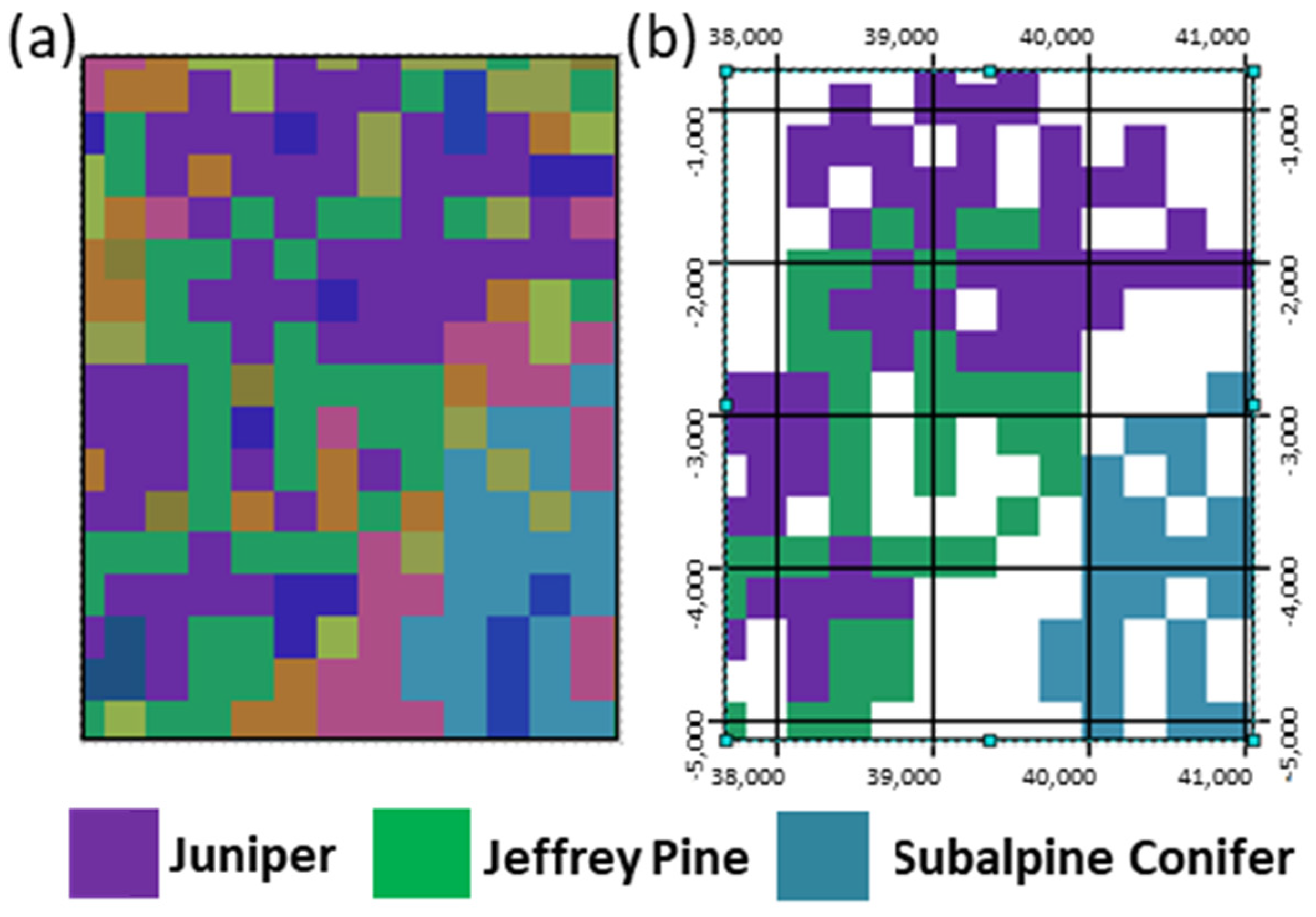
2.4. Development of Vegetation Type Map

We used a vegetation map developed by California’s Fire and Resource Assessment Program (CALFIRE; FRAP: https://resilientca.org/projects/1846ff66-187f-4865-a97a-38cad24bacf8/, accessed on 8 November 2012) [34]. This map compiled the most recent landcover maps across California into a single comprehensive statewide dataset. Crosswalks were used to compile the various sources into two classification schemes, the California Wildlife Habitat Relationships (CWHR; CDFW) [35], and the Macrogroup-level of the National Vegetation Classification (NVCS) system [36]. We used the CWHR classification for the subsequent steps. Our analysis regards only native vegetation, therefore areas defined as urban, irrigated agriculture of various types, orchards, vineyards, pasture, and rock and water bodies are not included in calculations.
The vegetation data were resampled from the original 30 m to 270 m to match the BCM. To be able to sample the 1-km ETa dataset using the vegetation map, it was necessary to identify groups of grid cells that represented vegetation types. This was performed using the Region Group tool in ArcGIS to identify connected regions of the same CWHR type, with any regions having less than 20 270-m cells (~1.5 km2) excluded (Figure 2). This enabled the sampling of the ETa maps using a vegetation map that best represented the AET of a single vegetation type.
We extended beyond the California state boundary to incorporate all inflowing drainages and used GAP/LANDFIRE National Terrestrial Ecosystems data land cover data [37] that incorporates NVCS to represent natural and semi-natural land cover types. A crosswalk was created between the MacroVeg groups in these areas and the CWHR classes based on descriptions and aerial imagery. There are 35 native CWHR vegetation types used in this analysis.

2.5. Calculation of Kv

To develop a mechanistic approach to transpiration, we extended the concept of crop coefficients to most natural California vegetation types. This method uses the concept of estimating AET given values of PET that are limited by a native crop coefficient, Kv (Howes and others 2015). Thus,
AET = Kv × PET
And conversely, the Kv is calculated as AET/PET for each month for each vegetation type. In this application, Kv = ETa/PET and it was calculated statewide for each month from 2000 to 2015 and the maps were sampled using the vegetation map to develop a 16-year monthly time series of Kv for each vegetation type.

2.6. Model Calibration to Match AET

Step 1 in the calibration was to average the 16 years of Kv estimates for each month and use those values in the BCM to scale the monthly estimates of AET with PET (Equation (1)) and calculate the AET for the 16-year time series of climate using the mapped soil depth. If the BCM-predicted AET for each vegetation type was lower than the ETa, the soil depth would be increased for each grid cell by 0.25 m until the difference between ETa and AET was no more than 5%. Although we know that roots penetrating into bedrock are accessing water in fractures and through mycorrhizal extraction to varying depths, for the purpose of this calculation and to quantify the volume of water being accessed we assume that the properties of the subsurface material being accessed by roots are the same as the soil properties; thus, we term this increase as an “effective” rooting volume or depth. At this step, the required soil depth represents our estimate of effective rooting depth. Step 2 was to account for the varying response to the precipitation of different vegetation types. Whereas Douglas fir forest changes its AET very little from year to year with varying precipitation, some vegetation types will respond readily to more or less precipitation, such as annual grasslands or oak woodlands. The model calibration allows for the addition of a precipitation scaler for each month that is multiplied by the Kv for that month. The more responsive a vegetation type is to precipitation variation, the more the scaler will deviate from 1.

2.7. Projecting Calibrated Landscape ET to Assess Drought Stress

To evaluate the range of hydrologic conditions that different vegetation types experience across their distribution in CA we used the variable climatic water deficit (CWD) to differentiate between the conditions experienced by Blue Oak Woodland/Blue Oak Foothill Pine (BOW/BOP) and Douglas fir (DFR). CWD is the evaporative demand that exceeds available water and is calculated monthly as AET minus PET and accumulated over a water year. The longer water is available in the soil profile, the higher the AET over the growing season and the lower the CWD. Depending on climate and energy balance conditions, increasing effective rooting depth could make vegetation more resilient to drought conditions.
We sampled the CWD for water year 2021, the second of 2 very strong drought years, calculated with and without using Kv and increased effective rooting depth to enable AET estimates from bedrock for every location mapped as BOW/BOP or DFR to describe the range of CWD they experienced that year and how the improved characterization may indicate vegetation responses to drought.

3. Results

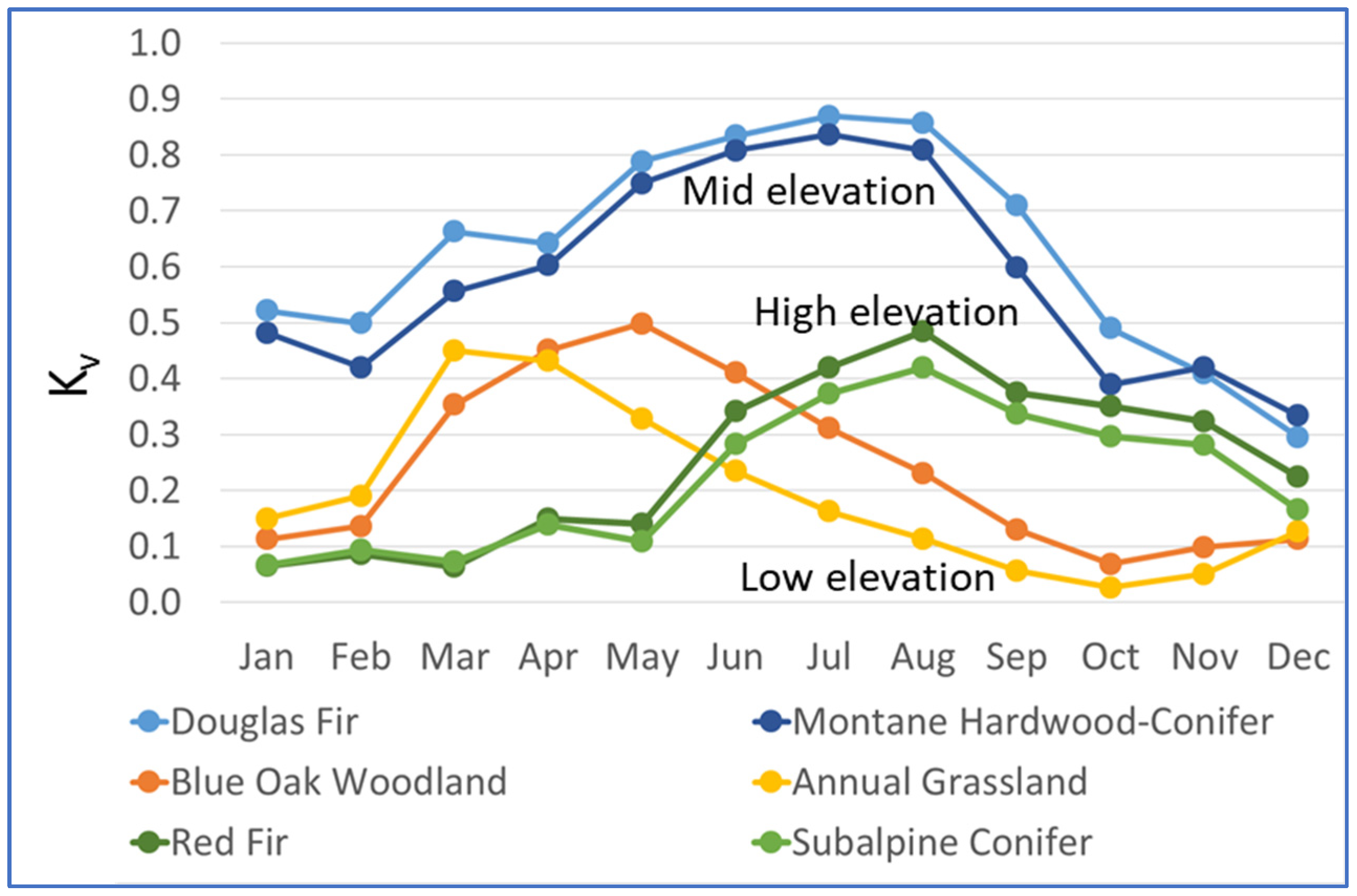
3.1. Kv Calculations

ETa for California, resampled to 270-m grid cell resolution, is shown in Figure 3a for June of 2012, and shows high values in the north coast and Sierra Nevada forested regions. PET calculated from the BCM for June 2012 (Figure 3b) and the spatially distributed Kv for the native vegetation is calculated as ETa divided by PET (Figure 3c) approximating the ratio of transpiration that would occur in the absence of water stress to the reference evapotranspiration of PET. Monthly Kv and soil depth added to achieve calibrated matches of AET to ETa are shown for 35 vegetation types in California (Table 1). The added soil depth values range from zero meters, generally for desert vegetation types, to 2.00 m for Douglas fir. Desert vegetation are generally in deep soils with low rainfall and did not require increases in soil depth to match the already low AET. Total effective soil depths (the original depth in the model plus the added depth) ranged from 0.7 for desert succulent shrubs to 3.1 m for annual grasslands.
Examples of monthly Kv values calculated for selected vegetation types are shown in Figure 4 for two low-elevation vegetation types, two mid-elevation, and two high-elevation vegetation types to indicate the seasonality of Kv that allows for AET when vegetation is driven by water availability or limited energy. Low-elevation vegetation types, annual grassland and blue oak woodland, which occupy warmer regions in the state with less precipitation, have their highest evapotranspiration in the spring when winter rainwater is still in the soil, and being relatively water-limited, have low ET rates, even at their peak seasonal growth, with Kv values about half of PET. High-elevation vegetation types, such as subalpine conifer and red fir, are energy limited, beginning their seasonal growth later into the season following snow melt, and maintaining their ET processes throughout the summer and late into the fall. These values represent the absence of water or temperature stresses, and while we assume the Kv value does not change for a given vegetation type under varying climate conditions, the calculated AET is responsive to monthly precipitation that deviates from the average as well as increases in evaporative demand with warming.

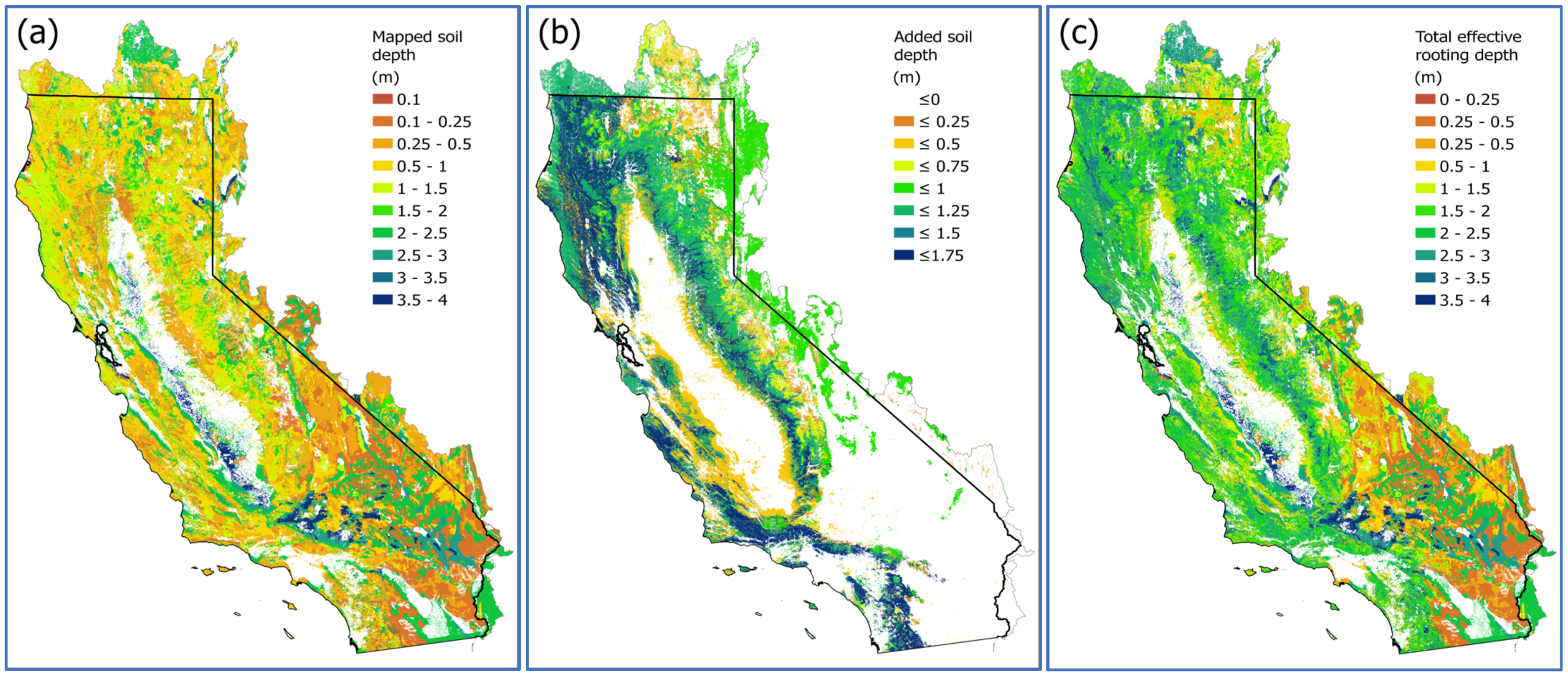
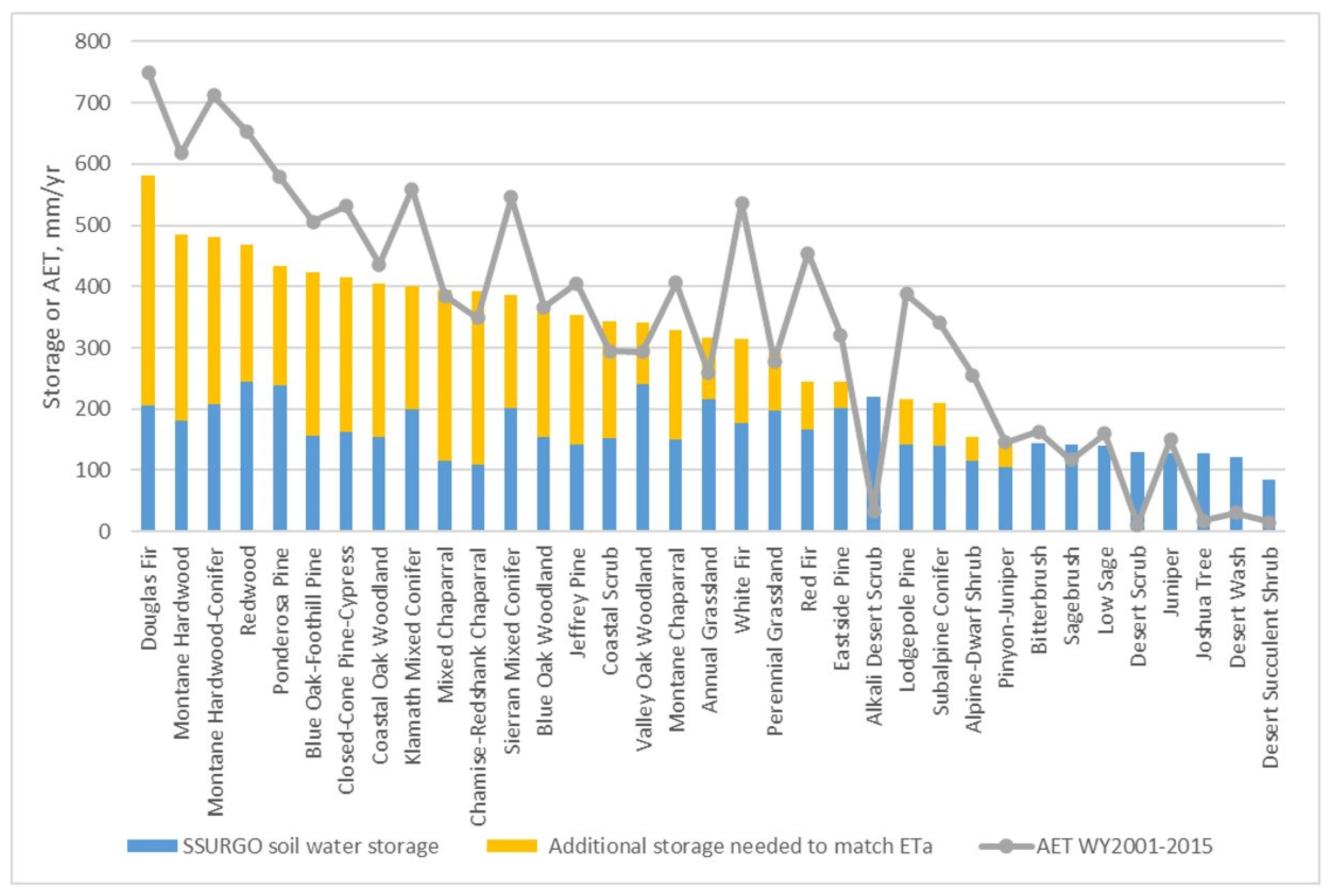
3.2. Effective Rooting Volume in Soil and Bedrock

An example of iteratively increasing soil depth is shown for Douglas fir (Figure 5), where the extracted ETa determined by Reitz et al. [26] is the dark black line and the AET calculated using the SSURGO soil depth is shown as the lower red line. Increasing the soil depth by 0.25 m increments results in a 2.00 m depth that is within 5% of the black line. This threshold value was chosen to not unreasonably increase the depth attempting to get a perfect match. Sixty percent of the vegetation types required additional soil depth in order to match ETa, for a maximum of 2.00 m added over an average depth from a SSURGO of 1.00 m, for a total maximum depth of 3.00 m (Table 1).
The mapped soil depth from SSURGO is shown in Figure 6a, excluding urban and irrigated locations. The vegetation parameters for Kv and increase in effective rooting depth are averaged for each vegetation type over the distributed soil properties for the state, which is illustrated in Figure 6b, to indicate the increase in rooting depth that incorporates water use from bedrock. The addition of these two maps creates an effective rooting depth map as shown in Figure 6c. The excess soil moisture storage needed to match ETa is primarily in the mid-elevation locations in the northwestern part of the state and in the western slope of the Sierra Nevada and southern California mountains. The highest addition of soil depth occurred in mid-elevation locations where there was more water available from precipitation but it was limited by the soil depth mapped. In southern CA this is dominated by the mixed chaparral and chamise redshank chaparral vegetation types. In northwestern CA, this is primarily Douglas fir, and in the Sierra Nevada foothills, it is dominated by the montane hardwood vegetation type. Calibration results for all vegetation types are detailed and described in Appendix A.
The average soil water storage needed to simulate actual evapotranspiration to match actual evapotranspiration, along with the average soil depth for each vegetation type is shown in Figure 7. The soil storage is the colored bars, whereas the average 2001–2015 AET is shown as the line with points. The graph is sorted by total soil depth, blue is soil and yellow is bedrock, with Douglas fir, montane hardwood, and montane hardwood conifer being the deepest. Chaparral has a high additional storage added, and there is no soil added for desert species in arid locations. The total storage is lower for most vegetation types than the AET because of seasonal precipitation occurring once soil water is removed, allowing for soil storage to be reached multiple times in the water year. Additionally, there is also uncertainty in the calibrations due to averaging vegetation types over the state, and local scale calibrations are recommended for local scale applications.

3.3. Comparisons of Model Simulation with and Without Kv Values and Addition of Effective Rooting Depth

Climatic water deficit (CWD; evaporative demand that exceeds available water, calculated as PET-AET) is an integrated indicator of hydrologic condition, and useful for modeling vegetation responses to changing climatic conditions across complex landscapes [2]. The BCM was run with vegetation-specific AET with the Kv and increased effective rooting depth (BCMv8), and without (BCMv65) [31] to calculate CWD. A close up of northern CA is shown in Figure 8 for water year 2021, a drought year following a drought year. Subtracting the BCMv65 CWD from the BCMv8 CWD illustrates where the CWD is reduced by including enhanced soil storage with bedrock storage and Kv, and therefore describes where vegetation may be more resilient to increases in CWD due to climate change by more realistically estimating water available from bedrock. The cool colors indicate where estimated plant water stress is lower than the modeled version without vegetation-specific evapotranspiration. The new model version better matches the satellite-based metrics of AET because of the use of an effective rooting depth. This is particularly true for the mid-elevation vegetation types that have the highest ET rates.
Targeting two vegetation types, blue oak woodland/foothill pine (BOW/BOP), a low elevation type, and Douglas fir (DFR), mid-elevation, we can see a much larger decline in CWD with increased effective rooting volume in Douglas fir than blue oak woodland/foothill pine (Figure 9A). We can also visualize the distribution of CWD for the two vegetation types in a drought year (Figure 9B). BOW/BOP has a very large range of CWD from 750 mm/year to double that in the southern part of its range. Douglas fir, however, has little impact from the drought, with some higher CWD values only in the south.

4. Discussion

The use of coefficients, Kv, that adjust average monthly AET below PET, effectively characterizes the spatial distribution of where vegetation types occur and how they use water seasonally. Incorporating an effective rooting depth to simulate a vegetation type’s access to water either below mapped soil depths or into bedrock to match measured AET improves the representation of native vegetation water use in California, more accurately illustrates where vegetation gets its water and how much is accessed in bedrock, and can provide some insights into the resilience of different landscapes to drought and climate change. The characterization of all mapped vegetation types provides a much fuller picture of the seasonal water use across the state. For example, only characterizing woody vegetation, although the biggest water user (Figure 7), does not include the early season water use by annual and perennial grasslands and grasses present in oak woodlands, that diminish the water available for the woody plants later in the season. The early season water users will often kick off the wildfire season in warmer than average springtime months.
Among woody vegetation types, we also found distinct elevational variation in the amount of water use. Vegetation types at mid-elevations, such as Douglas fir and montane hardwood-conifer in California, generally have the most water available for ET. They are not constrained by either summer drought at lower elevations or low temperatures found at the higher elevations, and thus can maintain higher ET rates throughout the year, and with nearly 95% of PET at their peak season. These results support the concerns described by Goulden et al. [38] that mid-elevation forests with the highest ET rates may move up in elevation with rising air temperatures and use far more water than high elevation vegetation types currently use, increasing stress on high elevation landscapes.
Vegetation types with higher than projected AET rates (Figure 7), when calculated across their range, can be better represented with the addition of soil depth that we term effective rooting depth. This represents the additional depth of soil required, assuming the same soil properties as mapped in SSURGO, to supply the water needed to match observed ETa. It is not a measure of actual rooting depths, as plant roots may penetrate soil layers with different water holding capacity as well as extending deep into fractured bedrock. In California, rooting depths have been observed up to 3.7 m in blue oaks and 2.5 m in Douglas fir [39,40], with temperate coniferous species ranging from 2 to 8 m [41], and as deep as 12 m anecdotally for coastal Douglas fir (T. Dawson, personal communication 2021). Vegetation types with the most soil water storage are in locations that are less water limited or energy limited. The AET is higher than the soil water storage for most vegetation types because most locations get multiple precipitation events over a year that are used by the plants and then replenished multiple times. The peaks in annual AET are generally for coniferous vegetation types, likely due to the greater leaf area that is maintained year-round and higher vegetation density.
Some vegetation types, especially in the deserts and grasslands, are responsive to precipitation events at time steps of days rather than months, exhibiting a facultative growth and AET response to precipitation [21]. These plants also exhibit stomatal resistance to water limitations. Mata-Gonzalez et al. [21] note that the crop coefficient Kc was designed for irrigated crops and assumes that plants are not subjected to resource limitations, including assumptions that plants have high leaf area and little stomatal resistance to water loss, and therefore, they concluded that the Kc method was not suitable for determining the AET of vegetation adapted to arid conditions. However, Howes et al. [42] used a vegetation coefficient Kv for the natural vegetation in California’s Central Valley for perennial grassland, native pasture, oak grassland, and semi-arid and arid chaparral. Our approach recognizes the limitation of a Kv developed based on a monthly ETa analysis and attempts to further characterize the water use of desert vegetation types that have sub-monthly responses to climate not reflected by our monthly time step by using a water balance approach to empirically adjust Kv upwards to match estimates of recharge and observed runoff but did not require an increase in effective rooting depth.
To achieve vegetation growth and the associated AET that occurs in the mid-elevation zones where there are less extreme water or energy limitations requires an increase in root exploration below the estimated soil depth from SSURGO, and likely into weathered bedrock or fractures [43]. This was explored by McCormick et al. [1], where they conclude that there is widespread use of water stored in bedrock by woody plants, whether in bedrock with high porosity or with fractures. The severe drought from 2013 to 2015 in California led to widespread die-off of the low and mid-elevation pines [7], suggesting that while the soils were notably dry, the water held in the bedrock had also been depleted, leading to increased tree mortality due to drought and increased susceptibility to pests and pathogens. Dieback was also observed in blue oak, and was more severe on hard granitic substrates, demonstrating the importance of substrate for climate resilience [44]. This reservoir of water deserves additional attention and the ability to include it in water balance modeling is critical.
Mid-elevation soils and bedrock accessed by vegetation for AET in California appear to be deeper than valley perimeter soils and certainly deeper than the highest elevation locations (Figure 6c). This enhanced soil development and weathering of shallow bedrock is likely due to available water for plant transpiration with corresponding root growth, and freeze/thaw processes with a rain/snow line as in the western flank of the Sierra and resulting in the adaptation of vegetation types to use water stored in deeper soils and weathered bedrock. Alternatively, the factors that lead to increased CWD (increased temperatures, earlier snowmelt, and/or decreased precipitation) may result in changes to vegetation type, composition, or structure as landscape vegetation adapts to more extreme conditions [2].
The use of CWD to help understand complex processes is limited by our understanding of interactions between water storage and the ability of plants to access deeper reservoirs of water [2,43], and trees in some montane areas may avoid deficits by tapping deeper reservoirs, a complexity not included in most current soil models. Refinements in CWD have been encouraged to better understand these complexities and to investigate the integrated effects of water balance on vegetation dynamics, which is critical to predict and manage vegetation responses to climate change [2].
The spatial and climatic distribution of conditions under which vegetation types occur can provide clues as to where they will be more or less at risk to succumb under extreme conditions, which regularly occur in the western US. Vegetation types at the edge of their climatic tolerances are the most at risk of failing to survive in a warming climate [45]. This is apparent in the blue oak-foothill pine CWD signatures in 2021 and could be evaluated for all widely distributed vegetation types. The varying distribution of climate change across the state, along with the distribution of soil and bedrock reservoirs for water, result in individualistic biogeographic responses [46]. The utility of characterizing the water use of landscapes and specific vegetation types can assist resource managers in prioritizing strategies for land management to produce healthy and resilient forests and lessen the likelihood of stressed vegetation and severe wildfire.
A particularly important aspect of quantifying the extraction of water from bedrock is the resulting increase in root zone deficit that is required to be filled prior to the initiation of runoff or recharge. For our vegetation types and hydrologic California footprint, the quantification of the bedrock water holding capacity increases available water from 67 MAF to 107 MAF, an increase of 40 MAF or 67% over that calculated by mapped soils alone (see Figure A4). This is supported by McCormick et al. [1], who used a far simpler water balance method but still determined that 16.2 MAF were extracted from bedrock in CA by woody plants alone and within state boundaries. An example of this occurred in California when, after the 2012–2016 drought, a doubled mean precipitation year did not lead to anticipated increases in runoff and the replenishment of reservoirs. Much of the melt in that year became recharge, replenishing soil moisture or shallow bedrock rather than surface reservoirs. The ability to forecast the dynamics of recharge vs. runoff has large implications for reservoir operators and water supply managers, and better estimates of how effective rooting depth and vegetation water use can mediate plant water access at landscape scales will help address this challenge. Conversely, accurately simulating antecedent soil moisture conditions, including shallow bedrock storage, can highlight where severe storms may result in excesses in runoff leading to flooding. Including disturbances to vegetation such as wildfire or forest management in the water balance, thus reducing AET and increasing soil moisture, also influences the fate of runoff and recharge and allows for a representation of the spatial distribution of conditions and processes that lead to widely varying hydrologic responses in the landscape to disturbance.

5. Conclusions

A refined representation of water balance variables was developed based on improving water use estimates of California native vegetation with the novel calculation of an effective rooting depth that provided additional water available for evapotranspiration from bedrock. This was performed by incorporating detailed vegetation information into the BCMv8 regional water balance model and calculating monthly scaling factors for each vegetation type to reflect the monthly ratio of actual to potential evapotranspiration. To match the measurements of average actual evapotranspiration for each vegetation type, we added an effective rooting volume iteratively as a depth increase to the soil depth maps to allow for quantifying the total available water for vegetation, including both soils and underlying bedrock water use resulting in a modified soil depth map that accounts for root exploration beyond the typical soil depth map. The resulting distinctions in AET by vegetation type along elevation and aridity gradients and for phenological cycles provide an innovative and valuable contribution to the studies of landscape ecology and plant water use and distribution.
An effective characterization of the components of landscape water balance is a critical factor leading to understanding the integrated effects of the water balance on vegetation dynamics, water movement and availability, and associated environmental responses to climate change. The use of climatic water deficit to focus on responses of vegetation to change and extremes has required refinements to ensure an accurate representation of the range of conditions plants can tolerate or thrive in. These depictions can aid in the interpretation of landscape scale patterns associated with climate to evaluate the best approaches for resource management.

Author Contributions

A.L.F. conceived of and developed the methodology, performed formal analysis and validation, wrote the model software, and contributed to original draft. L.E.F. designed the methodology, performed the formal analysis, validation, and visualization, wrote the original draft and revisions, and acquired funding. M.A.S. performed formal analysis and validation, contributed to the original draft and revisions, and curated the data. J.H.T. contributed to the formal analysis and original draft and review. R.B. contributed to the methodology. D.D.A. provided multi-disciplinary insights and manuscript review. All authors have read and agreed to the published version of the manuscript.

Funding

This research was funded by California Department of Water Resources under Agreement No. 4600011144 Am. 2 with the U.S. Geological Survey between 2018–2021.

Data Availability Statement

All model codes, control files, input layers and output layers, including a user’s manual are available on The Basin Characterization Model—A monthly regional water balance software package (BCMv8) data release and model archive for hydrologic California (ver. 3.0, June 2023)—ScienceBase-Catalog.

Acknowledgments

This work was conducted in collaboration with Pepperwood Preserve, California Department of Water Resources, the State of California Department of Conservation and Division of Land Resource Protection, with support from the California Coastal Conservancy, National Resource Conservation Service, and U.S. Geological Survey California Water Science Center. Thanks to Prahlada Papper, Sally Thompson, and Rob Skelton for instructive insights.

Conflicts of Interest

The authors Alan L. Flint and Lorraine E. Flint are employed by Earth Knowledge, Inc. The remaining authors declare no conflicts of interest. The funders had no role in the design of the study; in the collection, analyses, or interpretation of data; in the writing of the manuscript; or in the de-cision to publish the results.

Appendix A

A.1. Calculating Potential Evapotranspiration and Seasonality of Actual Evapotranspiration

The Basin Characterization Model has been revised to include soil organic matter (SOM) in the calculation of soil water holding capacity from texture, and vegetation type-specific actual evapotranspiration. Soil water holding capacity (WHC) from the Natural Resource Conservation SSURGO county-level map dataset [47,48] is calculated as water content at field capacity (FC, −0.03 MPa) minus water content at wilting point (WP, −1.5 MPa) multiplied by soil depth. These values are typically used for agricultural soils, whereas the BCMv8 use of texture (percent sand, silt, and clay) and soil organic matter allows us to better represent natural lands and increase WHC by increasing FC to −0.01 MP and WP to −6.0 MPa. Where SSURGO data is not available, STATSGO national data fills the gaps. Calculations of WHC are performed using equations from Saxton and Rawls [30], who evaluated the relation between soil texture, soil organic matter, porosity, FC, and WP based on thousands of laboratory-analyzed field samples. In valley locations with geology mapped as quaternary sediments, soil depth is extended to 4 m from the 2.01 m SSURGO limit.
Potential evapotranspiration (PET) is calculated based on a pre-processing program, SolPET [49] that simulates hourly solar radiation with topographic shading, atmospheric turbidity, ozone, and water vapor, and then uses the solar radiation and air temperature and a modified form of the Priestley-Taylor PET equation [50] with cloudiness [51] to calculate hourly PET. The Priestley-Taylor equation is as follows:
λ E a = α S S + γ ( R n G )
where E a is actual evapotranspiration, λ is the latent heat of vaporization, α is a model coefficient (which Priestley and Taylor allowed to vary for drying conditions), S is the slope of the saturation vapor density curve, γ is the psychrometric constant, Rn is net radiation, and G is soil heat flux. The equation used to develop the relationship between atmospheric transmittance (cloudiness) and air temperature [51] is as follows:
Tt = A [1 − exp(-BTC)]
where Tt is the daily total atmospheric transmittance, ∆T is the daily range of air temperature, and A, B, and C are empirical coefficients, determined for a particular location from measured solar radiation data. The coefficients have been determined for 85 stations active from 1980 to 2010 in the California Irrigation Management Information System (CIMIS; https://cimis.water.ca.gov/WSNReportCriteria.aspx, accessed on 4 April 2010), to develop average monthly gridded surfaces for each parameter for the PET calculation. An example calibration is shown with good matches to measured data (Figure A1).
Figure A1. Example calibration of potential evapotranspiration calculated by the BCMv8 to measured reference evapotranspiration from California Irrigation Management Information System (CIMIS) station data.
Hydrology 11 00211 g0a1
Some vegetation types are very responsive to annual changes in precipitation, such as annual grasslands, shown in Figure A2a, where the BCM AET is shown compared to ETa for 14 years. To simulate the range of variation in AET between years with more or less precipitation, parameters have been developed that use a scaler that is used to adjust the precipitation for each month in comparison to the long-term (here, 1981–2010) average monthly precipitation. This scaler is multiplied by the Kv for that month and is adjusted until the variability of the simulated AET matches ETa (Figure A2b). Examples of various vegetation types are shown in Figure A3 to illustrate the calibrated match of AET to ETa.
Figure A2. (a) Annual grasslands with no adjustments to growth parameters and (b) with growth parameters adjusted to match annual variability in precipitation.
Hydrology 11 00211 g0a2
Figure A3. Example fit of measured ETa and BCMv8 actual evapotranspiration for two vegetation types. The increase in plant available water that is calculated by incorporating bedrock water storage as available for vegetation AET is shown in Figure A4. This distribution of water highlights the western slope of the Sierra Nevada, the northwest part of the state and along the central coast.
Hydrology 11 00211 g0a3

A.2. Calibration Results of BCM to Actual Evapotranspiration, Streamflow, Baseflow Index, and Groundwater Flow Model Estimates of Recharge

Details of the model calibration process are in Flint et al. [27]. Results for the regional calibrations to various measured variables are included here to illustrate model validation with independent measured datasets.
In the regional calibration for California, 62 vegetation types were calibrated to the remote-sensing-derived ETa from Reitz et al. [26] for water years 2000–2015 and examples of calibrations for five vegetation types are shown in Figure A3. The entire dataset had an overall average R2 of 0.66 with better fits for vegetation in locations that were not water limited, such as medium to high elevation or north coast vegetation types, Sierran Mixed Conifer (R2 = 0.91), Ponderosa Pine (R2 = 0.84), or Redwood (R2 = 0.88). Vegetation types in water-limited locations had moderately good fits, such as Juniper (R2 = 0.68) or Mixed Chaparral (R2 = 0.51). Vegetation that responds to sub-monthly precipitation events and whose AET is therefore not represented well by the monthly time step of the measured data have poor fits, such as facultative desert species, Chamise-Redshank Chaparral (R2 = 0.27) or Low Sage (R2 = 0.39). Annual Grasslands have responses to sub-monthly precipitation events also (R2 = 0.61; Figure A2b), as well as vegetation types that include annual grasses (Blue Oak Woodland, R2 = 0.83), and calibrations were iteratively performed for some of these vegetation types to improve the match of recharge + runoff to measured streamflow data when there was more basin discharge calculated by the BCMv8 than there was measured streamflow. As a result of the AET calibration, the distribution of the available water that can be extracted by vegetation from bedrock is shown in Figure A4, indicating that additional water is available predominately in mid-elevation Sierra mountains, the northwest, and central coast regions.
Streamflow calibrations were performed iteratively by changing vegetation AET calibration parameters and bedrock conductivity to exactly match measured streamflow volumes for each period of available data for each of 55 streamgages and minimize the differences in the measured and modeled hydrographs to increase R2 and Nash-Sutcliff Efficiency (NSE) values. Examples of two streamgages are shown in Figure A5, illustrating the goodness-of-fit for a desert basin and a snow-dominated basin. Simultaneously minimizing the difference between the baseflow index calculated from the hydrograph separation method for all 55 gages resulted in an average R2 of 0.72 for all 55 basins and an NSE of 0.70. The same approach was taken for the 11 large water supply basins for which full natural flows are calculated in the Sierra Nevada and are the predominant source of California’s water supply. Because of the impairment in streamflow imposed by the reservoir operations, calculated full natural flows were used for calibration with an average R2 of 0.76 and NSE of 0.75.
Because the water balance is calculated monthly following the equation from Figure 1, any errors in all components of the BCMv8 process that have been individually calibrated are accumulated in the most uncertain variable being calculated, recharge, whether they result in baseflow from the post-processing to calculate basin discharge for streamflow calibration or are accumulated directly from the output maps used for groundwater flow model boundary conditions. The comparison of the baseflow index (BFI) derived from the BCMv8 and hydrograph separation method is shown in Figure A5a as a scatter plot. There is uncertainty in the hydrograph separation approach to calculating BFI in addition to regionally calibrating the BCMv8, and the approach of minimizing the difference in these values around the one-to-one line shows a fair amount of scatter. This approach allowed us to target large outliers to improve the fit. The calibration of the BCMv8 using all of these spatially distributed methods resulted in recharge estimates that compared well with empirically derived recharge boundary conditions for calibrated MODFLOW groundwater flow models in 26 basins across California (Figure A5b).
Figure A4. Distribution of the available water that can be extracted by vegetation from bedrock.
Hydrology 11 00211 g0a4
Figure A5. Examples of comparisons of basin discharge calculated by post-processing runoff and recharge calculated by the Basin Characterization Model version 8 to measured streamflow for (a) a desert basin on a log scale to illustrate low flows and (b) in a snow-dominated basin on a linear scale to illustrate matches to peak flows.
Hydrology 11 00211 g0a5
Figure A6. Calibration of BCMv8 to (a) the baseflow index calculated using baseflow separation methods and (b) estimates of recharge from Modflow groundwater flow models. Solid black lines are the 1:1 lines and dotted lines are linear regression lines.
Hydrology 11 00211 g0a6

References

  1. McCormick, E.L.; Dralle, D.N.; Hahm, W.J.; Tune, A.K.; Schmidt, L.M.; Charwick, K.D.; Rempek, D.M. Widespread woody plant use of water stored in bedrock. Nature 2021, 597, 225–229. [Google Scholar] [CrossRef] [PubMed]
  2. McIntyre, P.J.; Thorne, J.H.; Dolanc, C.R.; Flint, A.L.; Flint, L.E.; Kelly, M.; Ackerly, D.D. 20th century shifts in forest structure in California: Denser forests, smaller trees, and increased dominance of oaks. Proc. Natl. Acad. Sci. USA 2015, 112, 1458–1463. [Google Scholar] [CrossRef] [PubMed]
  3. Flint, L.E.; Flint, A.L.; Stern, M.A.; Mayer, A.; Silver, W.; Casey, C.F.; Franco, F.; Byrd, K.; Sleeter, B. Increasing Soil Organic Carbon to Mitigate Greenhouse Gases and Increase Climate Resiliency for California. Calif. Nat. Resour. Agency California’s Fourth Clim. Change Assess. Tech. Rep. 2018, CCCA4-CNRA-2018-006, 83p. Available online: https://pubs.usgs.gov/publication/70199846 (accessed on 10 November 2024).
  4. Tian, W.; Liu, X.; Liu, C.; Bai, P. Investigation and simulations of changes in the relationship of precipitation-runoff in drought years. J. Hydrol. 2018, 565, 95–105. [Google Scholar] [CrossRef]
  5. Hahm, W.J.; Dralle, D.N.; Sanders, M.; Bryk, A.B.; Fauria, K.E.; Huang, M.H.; Hudson-Rasmussen, B.; Nelson, M.D.; Pedrazas, M.A.; Schmidt, L.; et al. Bedrock vadose zone storage dynamics under extreme drought: Consequences for plant water availability, recharge, and runoff. Water Resour. Res. 2022, 58, e2021WR031781. [Google Scholar] [CrossRef]
  6. Park, I.W.; Mann, M.L.; Flint, L.E.; Flint, A.L.; Moritz, M. Relationships of climate, human activity, and fire history to spatiotemporal variation in annual fire probability across California. PLoS ONE 2022, 16, e0254723. [Google Scholar]
  7. Thorne, J.H.; Moody, T.; Rosenberg, M. Forest Tree Mortality. In Indicators of Climate Change in California; Milanes, C., Kadir, T., Lock, B., Miller, G., Monserrat, L., Randles, K., Eds.; California Environmental Protection Agency: Sacramento, CA, USA, 2022. Available online: https://oehha.ca.gov/media/04treemortality.pdf (accessed on 10 November 2024).
  8. Chen, J.; McGuire, K.J.; Stewart, R.D. Effect of soil water-repellent layer depth on post-wildfire hydrological processes. Hydrol. Proc. 2020, 34, 270–283. [Google Scholar] [CrossRef]
  9. Maina, F.Z.; Siirila-Woodburn, E.R.; Vahmani, P. On the sensitivity of meteorological forcing resolution on hydrologic metrics. Energy 2019, 7, 4–5. [Google Scholar]
  10. Thorne, J.H.; Boynton, R.M.; Flint, L.E.; Flint, A.L. The magnitude and spatial patterns of historical and future hydrologic change in California’s watersheds. Ecosphere 2015, 6. Available online: https://esajournals.onlinelibrary.wiley.com/doi/10.1890/ES14-00300.1 (accessed on 10 November 2024).
  11. Thorne, J.H.; Morgan, B.J.; Kennedy, J.A. Vegetation Change over 60 Years in the Central Sierra Nevada. Madroño 2008, 55, 223–237. [Google Scholar] [CrossRef]
  12. Goulden, M.L.; Bales, R.C. Mountain runoff vulnerability to increased evapotranspiration with vegetation expansion. Proc. Natl. Acad. Sci. USA 2014, 111, 14071–14075. [Google Scholar] [CrossRef]
  13. Ehlert, R.S.; Hahm, W.J.; Dralle, D.N.; Rempe, D.M.; Allen, D.M. Bedrock controls on water and energy partitioning. Water Resour. Res. 2024, 60, e2023WR036719. [Google Scholar] [CrossRef]
  14. Hahm, W.J.; Dralle, D.N.; Lapides, D.A.; Ehlert, R.S.; Rempe, D.M. Geologic controls on apparent root-zone storage capacity. Water Resour. Res. 2024, 60, e2023WR035362. [Google Scholar] [CrossRef]
  15. Hahm, W.J.; Rempe, D.M.; Dralle, D.N.; Dawson, T.E.; Lovill, S.M.; Bryk, A.B. Lithologically controlled subsurface critical zone thickness and water storage capacity determine regional plant community composition. Water Resour. Res. 2019, 55, 3028–3055. [Google Scholar] [CrossRef]
  16. Eggemeyer, K.D.; Schwinning, S. Biogeography of woody encroachment: Why is mesquite excluded from shallow soils? Ecohydrology 2009, 2, 81–87. [Google Scholar] [CrossRef]
  17. Cui, G.; Guo, W.; Goulden, M.; Bales, R. MODIS-based modeling of evapotranspiration from woody vegetation supported by root-zone water storage. Remote Sens. Environ. 2024, 303, 114000. [Google Scholar] [CrossRef]
  18. Doorenbos, J.; Pruitt, W.O. Crop Water Requirements; FAO Irrigation Drainage Paper 24 (Rev.); Food and Agriculture Organization of the United Nations: Rome, Italy, 1977. [Google Scholar]
  19. Allen, R.G.; Pereira, L.S.; Raes, D.; Smith, M. Crop Evapotranspiration–Guidelines for Computing Crop Water Requirements; FAO Irrigation Drainage Paper 56; Food and Agriculture Organization of the United Nations: Rome, Italy, 1998. [Google Scholar]
  20. Lascano, R.J. A general system to measure and calculate daily crop water use. Agron. J. 2000, 92, 821–832. [Google Scholar] [CrossRef]
  21. Mata-González, R.; McLendon, T.; Martin, D.W. The Inappropriate Use of Crop Transpiration Coefficients (Kc) to Estimate Evapotranspiration in Arid Ecosystems: A Review. Arid Land Res. Manag. 2005, 19, 285–295. [Google Scholar] [CrossRef]
  22. Wyatt, B.M.; Ochsner, T.E.; Zou, C.B. Estimating root zone soil moisture across diverse land cover types by integrating in-situ and remotely sensed data. Agric. For. Meteor. 2021, 15, 108471. [Google Scholar] [CrossRef]
  23. Klos, P.; Goulden, M.; Riebe, C.; Tague, C.; O’Geen, A.; Flinchum, B.; Safeeq, M.; Conklin, M.; Hart, S.; Berhe, A.; et al. Subsurface plant-accessible water in mountain ecosystems with a Mediterranean climate. WIREs Water 2018, 5, e1277. [Google Scholar] [CrossRef]
  24. Flint, A.L.; Childs, S.W. Physical properties of rock fragments and their effect on available water in skeletal soils. In Erosion and Productivity of Soils Containing Rock Fragments; Special Publication; Soil Science Society America: Madison, WI, USA, 1984; Volume 13, pp. 91–103. [Google Scholar]
  25. Ichii, K.; Wang, W.; Hashimoto, H.; Yang, F.; Votava, P.; Michaelis, A.; Nemani, R. Refinement of rooting depths using satellite-based evapotranspiration seasonality for ecosystem modeling in California. Agric. For. Meteor. 2009, 149, 1907–1918. [Google Scholar] [CrossRef]
  26. Reitz, M.; Sanford, W.E.; Senay, G.B.; Cazenas, J. Annual Estimates of Recharge, Quick-Flow Runoff, and Evapotranspiration for the Contiguous US Using Empirical Regression Equations. J. Amer. Water Resour. Ass. 2017, 53, 961–983. [Google Scholar] [CrossRef]
  27. Flint, L.E.; Flint, A.L.; Stern, M.A. The Basin Characterization Model version 8–A Regional Water Balance Software Package. U.S. Geol. Surv. Tech. Methods 2021, 6–H1, 85. [Google Scholar] [CrossRef]
  28. Daly, C.; Halbleib, M.; Smith, J.I.; Gibson, W.P.; Doggett, M.K.; Taylor, G.H.; Curtis, J.; Pasteris, P.P. Physiographically sensitive mapping of climatological temperature and precipitation across the conterminous United States. Inter. J. Climatol. J. R. Meteor. Soc. 2008, 28, 2031–2064. [Google Scholar] [CrossRef]
  29. Flint, L.E.; Flint, A.L. Downscaling climate change scenarios for ecologic applications. Ecol. Process 2012, 1, 1–15. [Google Scholar]
  30. Saxton, K.E.; Rawls, W.J. Soil water characteristic estimates by texture and organic matter for hydrologic solutions. Soil Sci. Soc. Am. J. 2006, 70, 1569–1578. [Google Scholar] [CrossRef]
  31. Flint, L.E.; Flint, A.L.; Thorne, J.H.; Boynton, R. Fine-scale hydrological modeling for climate change applications; using watershed calibrations to assess model performance for landscape projections. Ecol. Process. 2013, 2, 1–25. [Google Scholar] [CrossRef]
  32. Mu, Q.; Zhao, M.; Running, S.W. Improvements to a MODIS global terrestrial evapotranspiration algorithm. Remote Sens. Environ. 2011, 115, 1781–1800. [Google Scholar] [CrossRef]
  33. Senay, G.B.; Bohms, S.; Singh, R.K.; Gowda, P.H.; Velpuri, N.M.; Alemu, H.; Verdin, J.P. Operational evapotranspiration mapping using remote sensing and weather datasets: A new parameterization for the SSEB approach. J. Am. Water Resour. Assoc. 2013, 49, 577–591. [Google Scholar] [CrossRef]
  34. California Department of Forestry and Fire Protection. California Vegetation by Wildlife Habitat Relationship Type; 2015. Available online: https://www.fire.ca.gov/Home/What-We-Do/Fire-Resource-Assessment-Program/GIS-Mapping-and-Data-Analytics (accessed on 11 November 2024).
  35. California Department of Fish and Wildlife and California Interagency Wildlife Task Group. Standards and Guidelines for CWHR Species Models. California Wildlife Habitat Relationship System; Technical Report No. 31; California Department of Fish and Game: Sacramento, CA, USA, 2014.
  36. Federal Geographic Data Committee. National Vegetation Classification Standard, Version 2; FGDC Document Number FGDC-STD-005-2008; U.S. Geological Survey: Reston, VA, USA, 2008. Available online: https://fgdc.gov/standards/projects/vegetation/NVCS_V2_FINAL_2008-02.pdf (accessed on 11 November 2024).
  37. U.S. Geological Survey. Gap Analysis Project (GAP), GAP/LANDFIRE National Terrestrial Ecosystems. U.S. Geol. Surv. Data Release. 2016. Available online: https://www.sciencebase.gov/catalog/item/573cc51be4b0dae0d5e4b0c5 (accessed on 4 April 2013).
  38. Goulden, M.L.; Anderson, R.G.; Bales, R.C.; Kelly, A.E.; Meadows, M.; Winston, G.C. Evapotranspiration along an elevation gradient in California’s Sierra Nevada. J. Geophys. Res. Biogeosci. 2012, 117, 1–13. [Google Scholar] [CrossRef]
  39. Cannon, W.A. Specialization in vegetation and in environment in California. In Plant World; Wiley: Hoboken, NJ, USA, 1914; Volume 17, pp. 223–237. [Google Scholar]
  40. McMinn, R.G. Characteristics of Douglas-fir root systems. Can. J. Bot. 1963, 41, 105–122. [Google Scholar] [CrossRef]
  41. Canadell, J.; Jackson, R.; Ehleringer, J.; Mooney, H.; Sala, O.; Shulze, E. Maximum rooting depth of vegetation types at the global scale. Oecologia 1996, 108, 583–595. [Google Scholar] [CrossRef]
  42. Howes, D.J.; Fox, P.; Hutton, P.H. Evapotranspiration from natural vegetation in the Central Valley of California: Monthly grass reference-based vegetation coefficients and the dual crop coefficient approach. J. Hydrol. Eng. 2015, 20, 04015004. [Google Scholar] [CrossRef]
  43. Bales, R.C.; Hopmans, J.W.; O’Geen, A.T.; Meadows, M.; Hartsough, P.C.; Kirchner, P.; Hunsaker, C.T.; Beaudette, D. Soil moisture response to snowmelt and rainfall in a Sierra Nevada mixed-conifer forest. Vadose Zone J. 2011, 10, 786–799. [Google Scholar] [CrossRef]
  44. McLaughlin, B.C.; Blakey, R.; Weitz, A.P.; Feng, X.; Brown, B.J.; Ackerly, D.D.; Dawson, T.E.; Thompson, S.E. Weather underground: Subsurface hydrologic processes mediate tree vulnerability to extreme climatic drought. Glob. Change Biol. 2020, 26, 3091–3107. [Google Scholar] [CrossRef] [PubMed]
  45. Thorne, J.H.; Choe, H.; Boynton, R.M.; Bjorkman, J.; Albright, W.; Nydick, K.; Flint, A.L.; Flint, L.E.; Schwartz, M.W. The impact of climate change uncertainty on California’s vegetation and adaptation management. Ecosphere 2017, 8, e02021. [Google Scholar] [CrossRef]
  46. Rapacciuolo, G.; Maher, S.P.; Schneider, A.C.; Hammond, T.T.; Jabis, M.D.; Walsh, R.E.; Iknayan, K.J.; Walden, G.K.; Oldfather, M.F.; Ackerly, D.D.; et al. Beyond a warming fingerprint: Individualistic biogeographic responses to heterogeneous climate change in California. Glob. Change Biol. 2014, 20, 2841–2855. [Google Scholar] [CrossRef]
  47. Wieczorek, M.E. Area- and Depth-Weighted Averages of Selected SSURGO Variables for the Conterminous United States and District of Columbia. USGS Data Ser. 866 2014. Available online: http://water.usgs.gov/lookup/getspatial?ds866_ssurgo_variables (accessed on 3 June 2017).
  48. Wieczorek, M.E. STATSGO2 Area- and Depth-Weighted Averages of Selected STATSGO2 Variables. Sci. Base-Cat. 2015. Available online: https://www.sciencebase.gov/catalog/item/54b97608e4b043905e00fc9d (accessed on 3 June 2017).
  49. Flint, A.L.; Childs, S.W. Calculation of solar radiation in mountainous terrain. Agric. For. Meteorol. 1987, 40, 233–249. [Google Scholar] [CrossRef]
  50. Priestley, C.H.B.; Taylor, R.J. On the assessment of surface heat flux and evaporation using large-scale parameters. Mon. Weather Rev. 1972, 100, 81–92. [Google Scholar] [CrossRef]
  51. Bristow, K.L.; Campbell, G.S. On the relationship between incoming solar radiation and daily maximum and minimum temperature. Agric. For. Meteorol. 1984, 31, 159–166. [Google Scholar] [CrossRef]
Figure 1. Schematic describing water balance components employed in the BCMv8.
Hydrology 11 00211 g001
Figure 2. Example of vegetation type map at 270-m gridcell resolution with (a) all vegetation types, and (b) with vegetation types grouped to omit gridcells with fewer than 20 contiguous cells, overlaid with the 1-km grids of the actual evapotranspiration, ETa, maps [26]. White areas in (b) indicate no data where mixed forest vegetation types did not meet the criteria of at least 20 contiguous grid cells.
Hydrology 11 00211 g002
Figure 3. Study area domain in California with variables for June 2012, (a) actual evapotranspiration, ETa [26], (b) potential evapotranspiration, PET, and (c) Kv calculated as ETa/PET, with irrigated land masked in white.
Hydrology 11 00211 g003
Figure 4. Examples of evapotranspiration coefficient, Kv, averaged monthly for water years 2000–2015 for six vegetation types.
Hydrology 11 00211 g004
Figure 5. Simulations of actual evapotranspiration from the BCMv8 with adjustments of the effective rooting depth into bedrock needed to match average ETa. Example for Douglas fir is optimized at 1.75–2.00 m of bedrock storage added to mapped soil depth.
Hydrology 11 00211 g005
Figure 6. Maps of (a) soil depth from SSURGO, (b) increase in effective rooting depth to incorporate water use from bedrock (or below mapped soil depth), and (c) total effective rooting depth with soils and bedrock.
Hydrology 11 00211 g006
Figure 7. Bedrock water storage needed above soil storage to calibrate modeled AET (actual evapotranspiration) to match measured actual evapotranspiration.
Hydrology 11 00211 g007
Figure 8. Climatic water deficit for water year 2021 illustrating the differences in calculated values by subtracting CWD calculated using the BCMv8 with vegetation-specific actual evapotranspiration and including bedrock water use, from CWD calculated with BCMv65 with vegetation transpiring at potential and only soil water use.
Hydrology 11 00211 g008
Figure 9. Climatic water deficit (CWD) calculated for water year 2021 for Blue Oak Woodland/Foothill Pine (BOW/BOP) and Douglas fir (DFR) (A) using enhanced effective rooting depths and Kv illustrating differences in cumulative probability, with much lower CWD for Douglas fir, and (B) spatially distributed indicating a much larger range of conditions for BOW/BOP in this drought year.
Hydrology 11 00211 g009
Table 1. Monthly Kv (actual/potential evapotranspiration) and soil depth added in analysis for 35 vegetation types in California. Douglas Fir (DFR) and Blue Oak Woodland/Blue Oak-Foothill Pine (BOW/BOP) are highlighted in bold for reference.
Vegetation TypePercent of AreaAdded Soil Depth (m)Monthly Kv Coefficients
OctNovDecJanFebMarAprMayJunJulAugSep
Alkali Desert Scrub2.70.000.0660.0860.1250.1420.1930.4450.5680.6260.5160.3910.2900.164
Alpine-Dwarf Shrub0.10.250.2140.1390.0480.0770.2120.2620.4260.3650.3400.2130.1970.227
Annual Grassland9.02.000.2190.1760.3080.2460.6580.8580.8300.6810.6010.5760.0630.358
Bitterbrush0.50.000.0220.1370.3020.3030.2070.3420.1840.1910.2220.1700.0980.036
Blue Oak Woodland2.31.300.0780.1200.1730.1880.2060.5330.6500.7340.5820.4670.3420.189
Blue Oak-Foothill Pine0.81.250.1210.1310.1230.1700.1490.3370.4480.6210.5580.4960.4130.276
Chamise-Redshank Chaparral1.12.100.1700.1800.2500.3200.4100.7600.7900.8800.9100.800.7000.520
Closed-Cone Pine-Cypress0.11.500.4150.3480.2330.4170.5100.6760.7220.8970.9490.8750.8190.627
Coastal Oak Woodland1.11.250.1300.2270.3110.3820.3520.4910.5150.4880.4210.3270.2700.158
Coastal Scrub1.51.500.0590.0620.1460.1770.2110.3530.3460.3070.2620.2300.1710.097
Desert Scrub19.61.000.4400.3400.3710.2440.2740.4860.5040.7140.8400.8400.7140.645
Desert Succulent Shrub0.10.000.0010.0050.0120.0230.0260.0560.0210.0050.0020.0020.0040.006
Desert Wash0.71.500.0430.0420.1970.2240.1290.2310.1840.1880.2170.2150.1890.119
Douglas Fir2.72.000.4960.4570.3390.5560.5210.6930.6470.7970.8200.8740.8640.717
Eastside Pine2.10.500.0670.1820.1880.3420.2720.4490.3300.3900.3710.3740.3210.167
Jeffrey Pine0.41.500.0020.0860.1310.2720.2210.4490.3950.4350.4280.4500.4090.288
Joshua Tree0.81.800.6250.5660.1660.4040.3380.6580.5740.6040.6290.6250.6250.625
Juniper0.91.500.0140.1310.1330.2300.2160.2830.1850.2770.2150.1620.0900.032
Klamath Mixed Conifer2.21.000.2800.2360.2040.3920.3530.5470.5440.640.06200.6960.6680.533
Lodgepole Pine0.40.750.0830.1440.1260.1910.1510.4280.5690.6130.4380.4190.4030.239
Low Sage1.0.400.0400.0520.0280.0990.0920.1910.303.01360.1060.1110.1090.086
Mixed Chaparral4.60.750.1260.1070.1720.2220.2570.4370.4720.5760.5510.4820.3790.245
Montane Chaparral1.50.750.0960.1360.1410.2240.1850.3630.3810.5060.4840.5040.4360.276
Montane Hardwood3.21.000.2700.2240.1580.2270.2820.4710.5340.7410.7580.7180.6520.471
Montane Hardwood-Conifer2.51.250.3980.4720.3790.5330.4480.5890.6100.7550.7930.8320.8030.609
Perennial Grassland0.30.750.0340.1050.1270.2270.2420.3770.2980.3770.3140.2770.1930.099
Pinyon Juniper2.21.200.0340.0440.1180.1730.1520.2480.1480.2180.2250.2120.1570.077
Ponderosa Pine0.61.400.2140.1710.1160.2320.2730.4770.437.03090.6310.6460.6070.472
Red Fir1.20.750.1010.1330.1210.2120.1930.4820.591.06890.5200.5130.4780.324
Redwood1.1.400.4850.4740.3630.4380.4750.5650.5610.6680.71.07770.8070.657
Sagebrush5.91.500.0170.1380.2980.0340.2660.8380.9000.8900.8810.4870.6860.619
Sierran Mixed Conifer3.90.500.2060.1670.1470.2820.3080.5540.4910.5800.5690.5940.5820.455
Subalpine Conifer0.90.750.0890.1220.0980.1630.1250.3470.4620.5290.4100.3940.3780.215
Valley Oak Woodland0.10.750.0630.0580.0870.0930.1080.2180.2670.363.03170.2750.2120.132
White Fir0.80.750.2120.2020.1740.3910.3670.6330.6000.6570.5680.6220.6070.474
Disclaimer/Publisher’s Note: The statements, opinions and data contained in all publications are solely those of the individual author(s) and contributor(s) and not of MDPI and/or the editor(s). MDPI and/or the editor(s) disclaim responsibility for any injury to people or property resulting from any ideas, methods, instructions or products referred to in the content.

