Investigating Induced Infiltration by Municipal Production Wells Using Stable Isotopes of Water (δ¹⁸O and δ²H), Four Mile Creek, Ohio

Abstract

Many municipalities around the world place their production wells in shallow alluvial aquifers that are adjacent to streams. Pumping these wells then induces the infiltration of surface water into the aquifer, allowing the greater extraction of water without significantly depleting the aquifer. However, induced infiltration poses a risk of introducing contamination from surface water into groundwater systems. The goal of this study was to quantify the amount of induced infiltration due to municipal pumping at the Four Mile Creek well field in Oxford, Ohio, using stable isotopes of water oxygen (δ¹⁸O) and deuterium (δ²H). In areas of municipal pumping, we sampled water from the production wells, Four Mile Creek, and from monitoring wells that we hypothesized to be both influenced and not influenced by induced infiltration. Samples were collected over 10 months in 2012 and over 12 months in 2021. In 2012, surface water δ¹⁸O values ranged from −3.89 to −8.04‰, and δ²H ranged from −26.55 to −55.65‰ at sampling sites. PW1 δ¹⁸O values ranged from −4.71 to −7.39‰ with a mean of −6.61 and −32.01 to −47.86‰ with a mean of −42.74‰ for δ²H. PW2 δ¹⁸O values ranged from −5.74 to −7.34‰, with a mean of −6.45‰, and δ²H ranged from −36.29 to −47.82‰ with a mean of −42.43‰. PW3 had lower values of both δ¹⁸O and δ²H, ranging from −6.36 to −8.02‰ and −47.7 to −40.35‰, and with means of −7.08 and −45.11, respectively. In 2021/2022, surface water δ¹⁸O values ranged from −5.32 to −7.93‰, and the δ²H ranged from −36.14 to −50.56‰. PW1 δ¹⁸O values ranged from −6.15 to −7.54‰ with a mean of −7.13‰, and δ²H ranged from −43.52 to −49.01‰ with a mean of −45.99‰. PW2 δ¹⁸O values ranged from −5.72 to −7.34‰, with a mean of −6.70‰, and δ²H ranged from −36.69 to −46.14‰, with a mean of −43.61‰. Using the time averaged values of δ¹⁸O of groundwater, production wells and surface water, the percentages of surface water resulting from induced infiltration in 2012 were 57%, 59% and 15% at the three wells, respectively, while in 2021, PW1 had 35% and PW2 91%. The amount of induced infiltration was apparently related to the pumping rates of the production wells, the length of time of pumping and the distance between Four Mile Creek and production wells. Our results indicate that stable isotopes of water provide a reliable method of quantifying groundwater/surface water interaction in alluvial aquifers.

1. Introduction

Understanding and quantifying groundwater and surface water interaction is important for sustainable water management and for the betterment of both humans and ecosystems [1,2]. For example, groundwater extraction that exceeds natural recharge rates may result in the reduced base flow of nearby streams [2,3]. A common source of drinking water supply throughout the world is represented by alluvial aquifers that are hydraulically connected to surface water bodies [4]. The often-high permeability of the alluvial aquifer sediment and high aquifer-recharge rates associated with induced infiltration from the surface water body both help minimize the drawdown in these production wells [5,6]. The water tables in alluvial aquifers are often shallow, and this allows for ease in groundwater withdrawal. There are, however, two potential problems with induced infiltration. First, the excessive withdrawal of groundwater from the aquifer near surface water can result in streamflow depletion [7]. Such flow reduction can have negative consequences for the local ecosystems [8] and for human populations that live downstream, especially in semi-arid and arid areas. The continued pumping of wells located near surface water may not only reduce streamflow in nearby drainages [9], but also lower the water table, reducing the discharge to adjacent water bodies and wetlands [10]. The second potential problem with induced infiltration is that surface water contaminants can be pulled into groundwater systems and may negatively affect water quality and cause health concerns [11,12]. The mixing of groundwater and surface water changes the chemical composition, acidity, temperature and dissolved oxygen content of the water, all of which are major controlling factors of aqueous geochemistry. It is therefore important to understand the effects of pumping on groundwater/surface water interactions, and to be able to quantify the amount of extracted groundwater that comes from induced infiltration.

Environmental isotopes of oxygen and hydrogen are widely used to understand many hydrological processes. Oxygen and hydrogen are part of the water molecule, and hence their isotopes are conservative along the groundwater flow path and not easily altered by water–rock interactions, making them ideal for tracing water sources [13]. Variations in the stable isotopic values of oxygen (δ¹⁸O) and hydrogen (δ²H) have been used to investigate hydrological conditions, moisture source conditions and precipitation trends [13,14]. Variation in isotopic values occurs because of fractionation due to thermodynamic processes during evaporation and condensation [4], and the degree of fractionation is dependent on temperature [15]. If groundwater is recharged from the infiltration of precipitation, then the groundwater isotopic composition will be similar to that of the local precipitation [16], with possible deviations resulting from evaporation after the precipitation event [4]. Subsequent studies have also used the stable isotopes of water to understand groundwater recharge and surface–water interactions [17,18]. In a study in La Crosse, Wisconsin, Hunt et al. [19] used stable isotopes of water to estimate the amount of municipally pumped groundwater that originated as induced infiltration. They based this on the idea that groundwater recharge was concentrated in the winter, and therefore the δ¹⁸O and δ²H values of groundwater were lower and less variable than the averages for surface water. Hunt et al. [19] applied a simple binary mixing calculation using the δ¹⁸O and δ²H values of surface water and groundwater to estimate the amount of surface water produced by the municipal wells.

This study applied the methodology of Hunt et al. [19] to characterize and quantify the average proportion of water from induced infiltration collected by each of three municipal wells in Oxford, Ohio. The methodology is based on the assumption that groundwater recharge in this part of the USA occurs primarily in the winter due to lower rates of evapotranspiration. Winter precipitation is characterized by lower isotopic values of δ¹⁸O and δ²H. We therefore expect that groundwater that is not affected by induced infiltration will have relatively low isotopic values no matter what season it is sampled. Surface water, on the other hand, will have isotopic values that vary much more throughout the year, and will therefore have higher time-averaged isotopic values. We hypothesize that a time-averaged proportion of water coming from induced infiltration could be quantified using δ¹⁸O and δ²H signatures of surface water, groundwater and municipal water, and a simple binary mixing model. The proportion of induced infiltration depends on the complex interactions of proximity to the surface water, pumping rates and underlying geology; however, the quantification of that proportion using a binary mixing model does not depend on knowing any of those factors. The specific research objectives for this study included: (1) measuring δ¹⁸O and δ²H values of surface water, groundwater not affected by induced infiltration and water produced from the municipal wells, and (2) using the means and standard deviations of isotopic values to quantify the degree of mixing between surface water and groundwater, and estimating the amount of water produced by the induced infiltration of surface water.

1.1. Background

Study Site Description

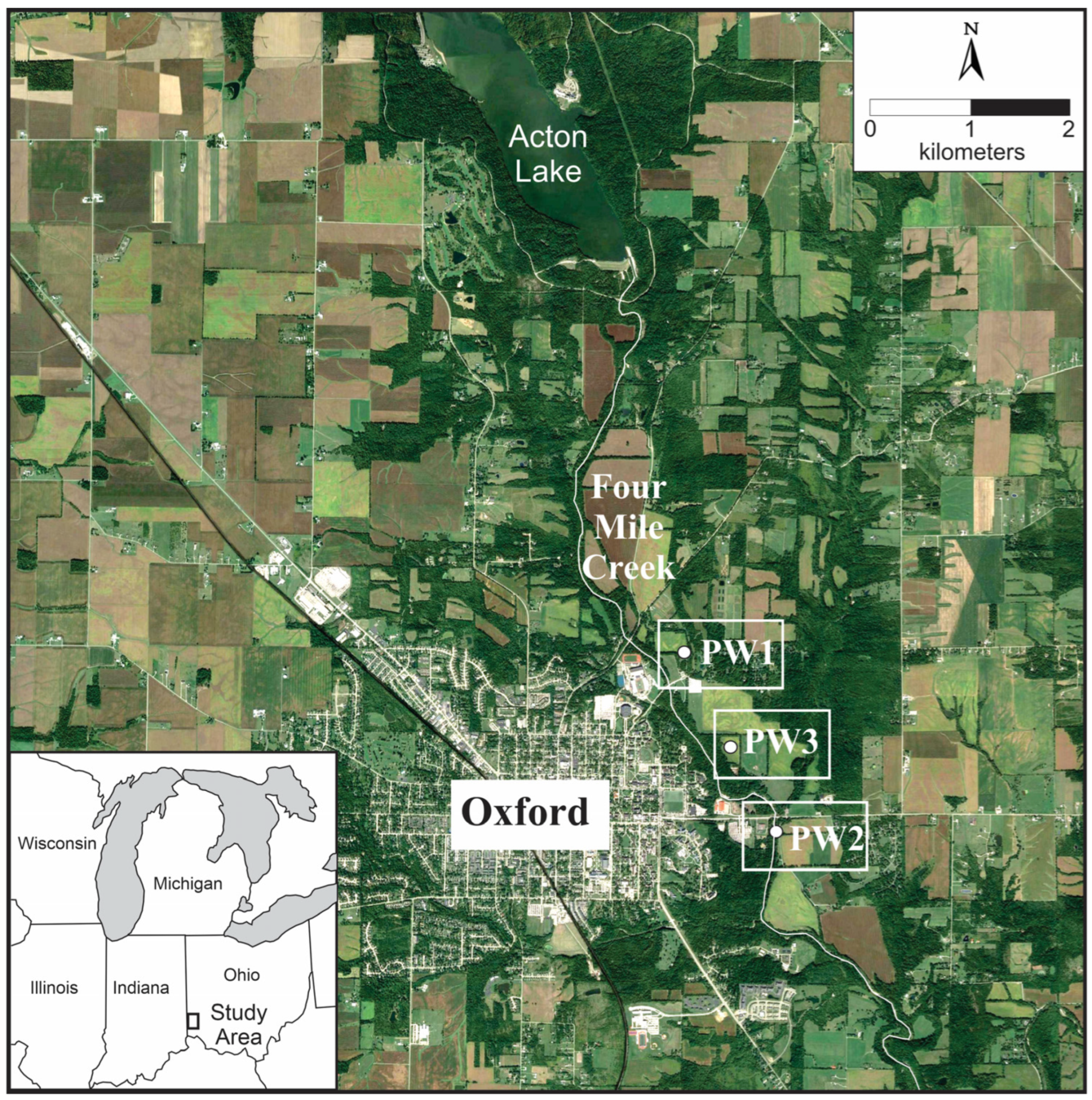
This study focused on an aquifer used to provide the municipal water of the City of Oxford in western Butler County in southwest Ohio, USA (Figure 1). The bedrock in this area comprises flat-lying, Ordovician-aged calcareous shale with interbedded layers of limestone, 0.03 to 0.1 m thick [20,21]. The bedrock’s permeability is too low to extract enough water for a municipal water supply. Instead, groundwater is pumped from glacial outwash sand and gravel deposited along with lacustrine silts and glacial tills during the Wisconsin glaciation in pre-existing river valleys [22,23]. Oxford’s Municipal wells are set in the Four Mile Creek valley, a tributary of the Great Miami River. Four Mile Creek flows from northwest to southeast. Oxford also utilizes supplemental wells in Seven Mile Creek valley, 12 km east of Oxford. Together, the Four Mile Creek and Seven Mile Creek wellfields serve a population of ~22,500 people in Ohio. The glacial outwash in Four Mile Creek valley is found just below a 0.5 to 2.0 m-thick layer of soil and fluvial overbank deposits. The outwash extends to a maximum depth of about 16 m. Everywhere in the valley, the glacial outwash is underlain by a layer of thick and relatively impermeable clayey glacial till forming the bottom of the aquifer [24]. The municipal wells were placed where the glacial outwash sediment is >10 m thick and laterally continuous [25].

The Four Mile Creek wellfield consists of three municipal wells, PW1, PW2 and PW3 (Figure 1). PW1 and PW2 are radial collector wells. PW1 is 200 m east of Four Mile Creek. It consists of a 3 m-diameter caisson that extends to the glacial till, 14 m below the ground surface, with six horizontal radial arms running in all directions 0.6 m above the till. On average, PW1 pumps about 1.3 × 10⁶ m³/y of water. PW2 is only 25 m west of Four Mile Creek and has a 3 m-diameter caisson that extends 12.6 m below the ground surface. It has three horizontal radial arms between 11 m and 12 m below the ground surface. These arms run west, away from Four Mile Creek. PW2 pumps about 9 × 10⁵ m³/y of water. PW3 is a conventional/vertical well, screened from 13.3 to 14.3 m below the ground surface, and is located 230 m east of Four Mile Creek. PW3 pumps about 7 × 10⁵ m³/y of water. 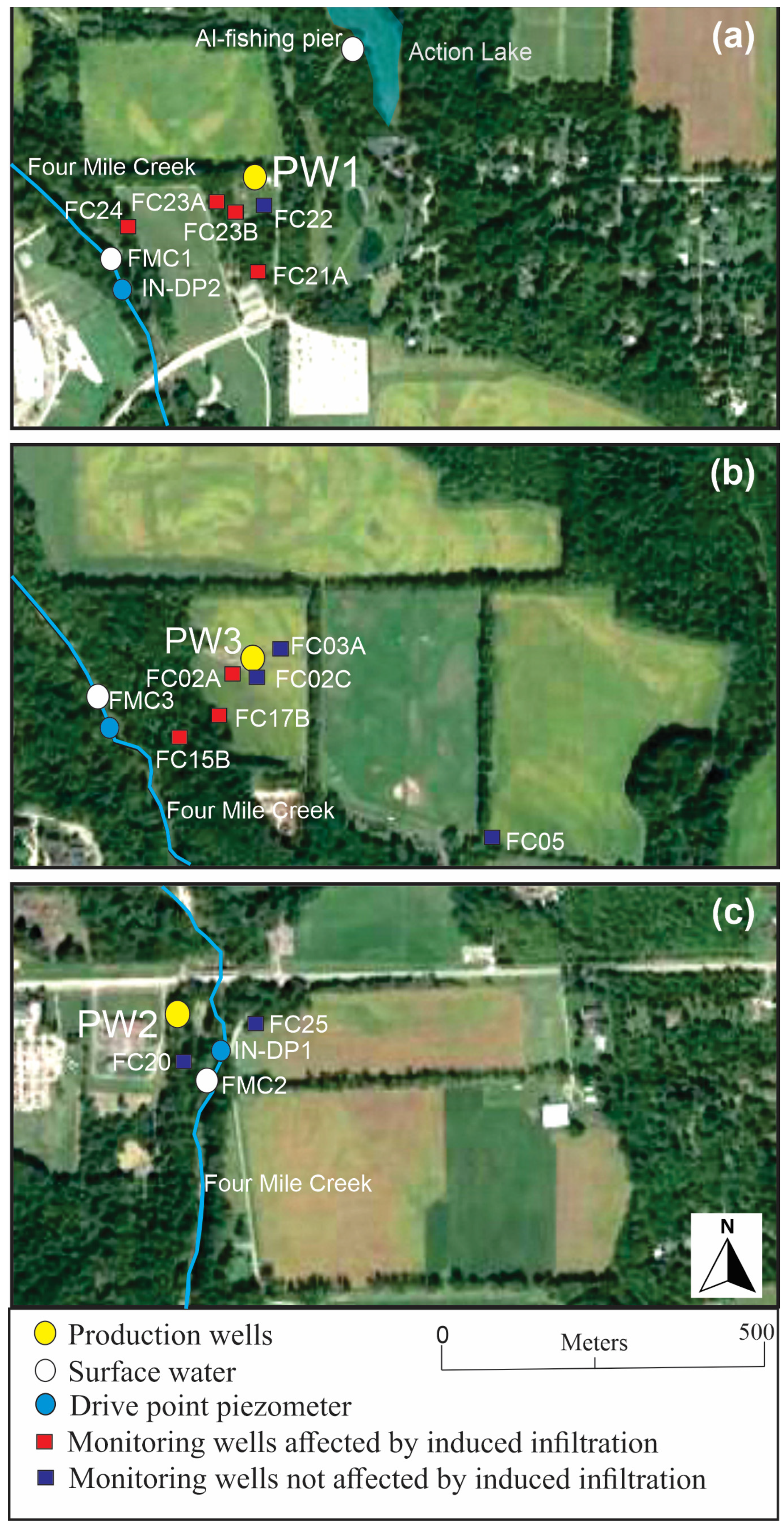Although these wells have a combined design capacity to pump 25,740 m³ of water per day, currently they pump an average of 8327 m³/d. PVC piezometers, either 0.051 m or 0.032 m in diameter, have been installed in the vicinity of each production well (Figure 2). Most have 1.52 m-long well screens set at various depths from the water table to the bottom of the aquifer (i.e., the top of the till). In addition, 0.032 m diameter drive-point piezometers with a 0.61 m-long well screen were installed in Four Mile Creek, 2 to 4 m below the creek bed, at locations in the creek closest to each of the production wells.

1.2. Groundwater Flow Directions and Hydraulic Gradients

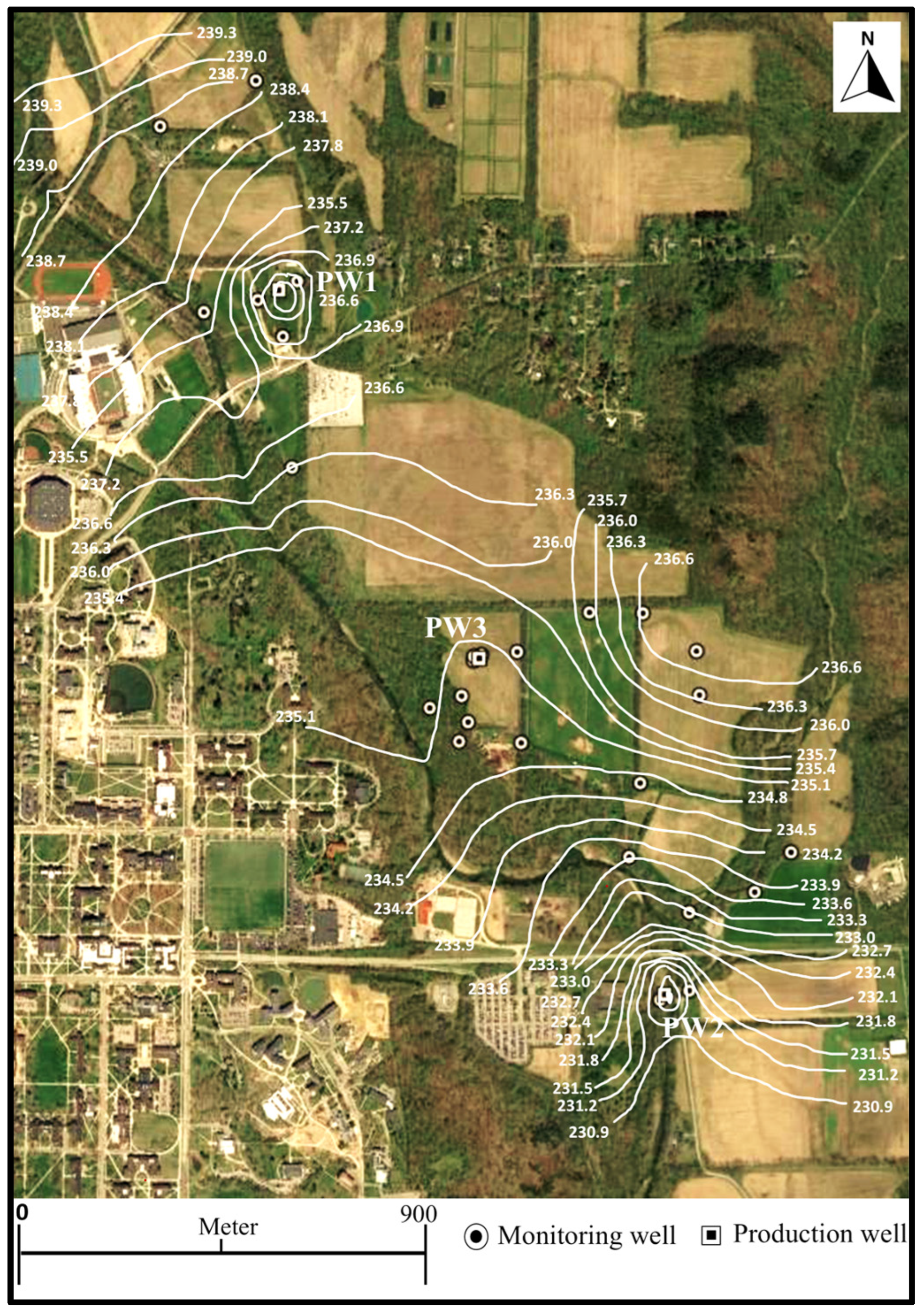
The groundwater flow directions were determined from water table maps, one of which is shown for conditions during October 2018 (Figure 3). There are cones of depression associated with each production well, with the deeper cones being at the radial collector wells, PW1 and PW2. Water table elevation contours indicate that Four Mile Creek is predominantly a gaining stream further away from the production wells, but a losing stream close to the production wells. Hydraulic gradients between the surface water and the groundwater beneath the streambed were measured continuously at the drive-point piezometers. The hydraulic gradients between the stream and the aquifer fluctuated as a result of varying stream flow and the different well pumping rates throughout the year. The gradients were consistently downward at all three stream locations nearest the production wells, indicating that pumping does induce infiltration and causes the creek to lose water to the groundwater system. The stream area near PW1 had the strongest downward gradients. These gradients ranged between 0.4 and 0.6 with the gradients increasing and decreasing in direct response to the pump turning on and off. At PW2, there is a confining clay lens that separates the stream from the underlying aquifer. As a result, when PW2 pumps, the water table drops below the bottom of the creek bed. There is a downward gradient, but without a hydraulic connection between the creek and aquifer. Infiltration may still be induced, but probably comes primarily from where the clay lens is not present. In Four Mile Creek, closest to PW3, gradients were again always downward, and ranged between 0.33 and 0.37. Unlike near PW1, gradients did not respond strongly to PW3 being turned on and off.

Based on the horizontal hydraulic gradients, we identified monitoring wells in the path of water traveling from Four Mile Creek to the production wells (Figure 2). These monitoring wells were designated as those to be affected by the induced infiltration of surface water. The monitoring wells assumed to be not affected by induced infiltration are those on the opposite sides of the production wells to Four Mile Creek.

1.3. Isotopic Composition of Precipitation in Southwest Ohio

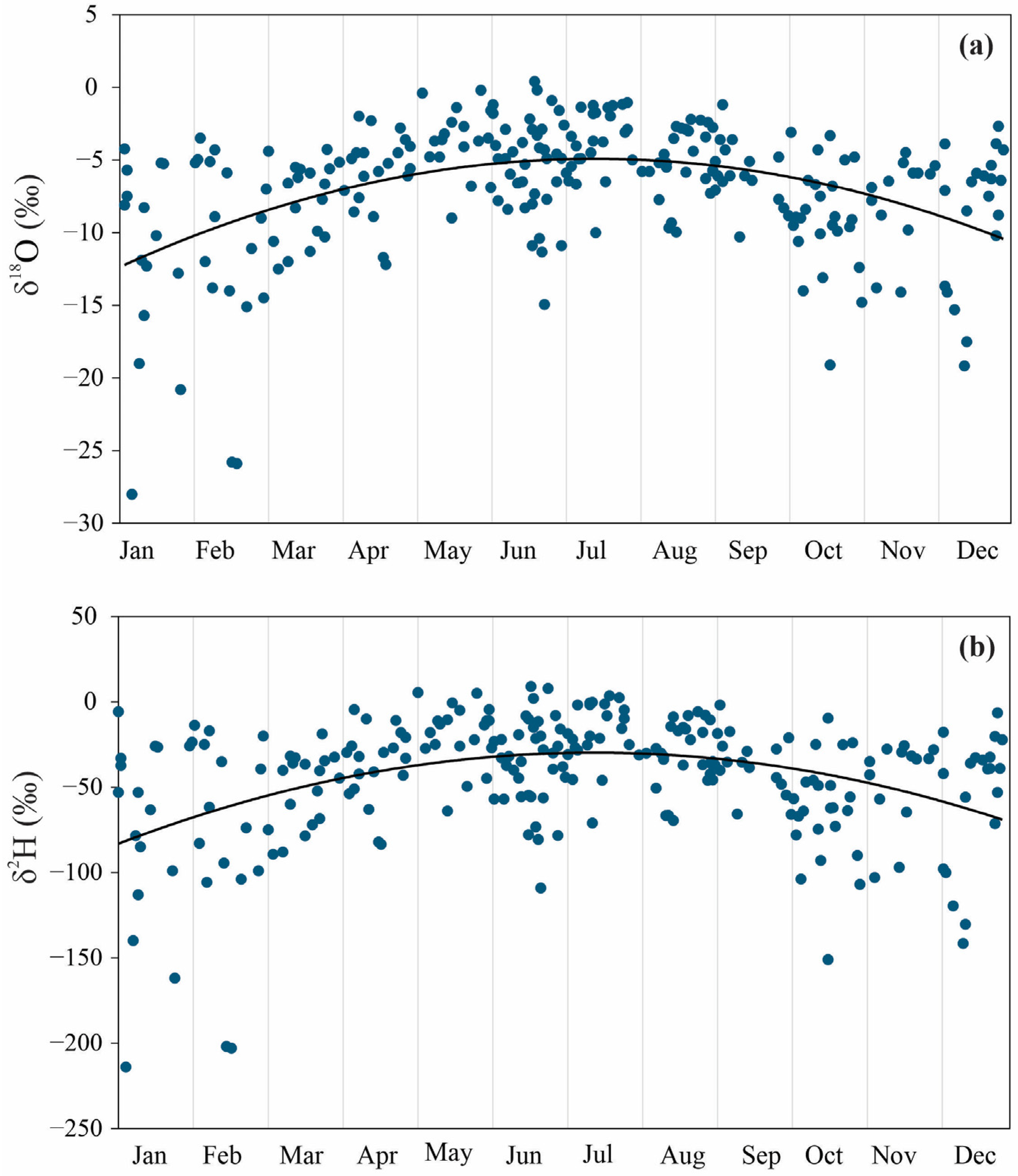
The isotopic composition of precipitation in southwest Ohio varies seasonally (Figure 4). Summer isotopic values for δ¹⁸O range from 0.4 to −10.9‰ VSMOW and average −5.5‰, while δ²H values range from 9.0 to −77.9‰ and average −33.7‰ VSMOW. Winter precipitation isotopic values are lower: δ¹⁸O ranges from −2.7 to −28‰ with a mean of −8.8‰, and δ²H ranges from −5.7 to −214‰ with a mean of −56.8‰ [14]. The observed variations in the isotopic composition of precipitation are mainly due to temperature fluctuations and moisture sources [26]. Other factors such as relative humidity and precipitation amount were not found to have a significant effect on the seasonal isotopic composition of precipitation in southwest Ohio [26]. Based on the seasonal variability exhibited in Figure 4, and our assumption that groundwater recharge happens primarily in the winter, we assume that the time-averaged isotope values of groundwater not affected by induced infiltration would be relatively low.

Variability in the isotopic composition of precipitation is partly due to the different sources of precipitation. The sources of precipitation in southwest Ohio are mid-latitude continental, Gulf of Mexico, Arctic Ocean, and the Pacific Ocean, each with different isotopic compositions and seasonal variations [26,27]. To describe the different sources, we cite only the δ¹⁸O values here, although the patterns are the same for δ²H values. The continental source precipitation has the highest annual average of −5.6‰. It is the most dominant in spring, summer and fall, when the respective average δ¹⁸O values are −7.4‰, −4.4‰ and −6.5‰. Precipitation from the Pacific Ocean occurs most in winter with a δ¹⁸O value average of −8.4‰. Pacific Ocean source precipitation has a more moderate annual average of −7.50‰. The Arctic source precipitation has a lower annual average δ¹⁸O value of −8.2‰, but also has the greatest seasonal variability. The Gulf of Mexico source precipitation has an intermediate annual average δ¹⁸O value of −7.58‰ [14]. During summer, the Gulf of Mexico precipitation is the most depleted due to the rainout effect and convective activity.

2. Materials and Methods

2.1. Sample Collection and Stable Isotope Analysis

Water samples were collected in two distinct periods: 2012 and 2021/2022. During both periods, surface water samples were collected from Four Mile Creek and groundwater samples were collected from the municipal production wells, monitoring wells and creek piezometers (Figure 1). The monitoring wells sampled for groundwater were chosen to represent wells that were identified as affected by the induced infiltration of surface water during pumping and those that were not affected by induced infiltration.

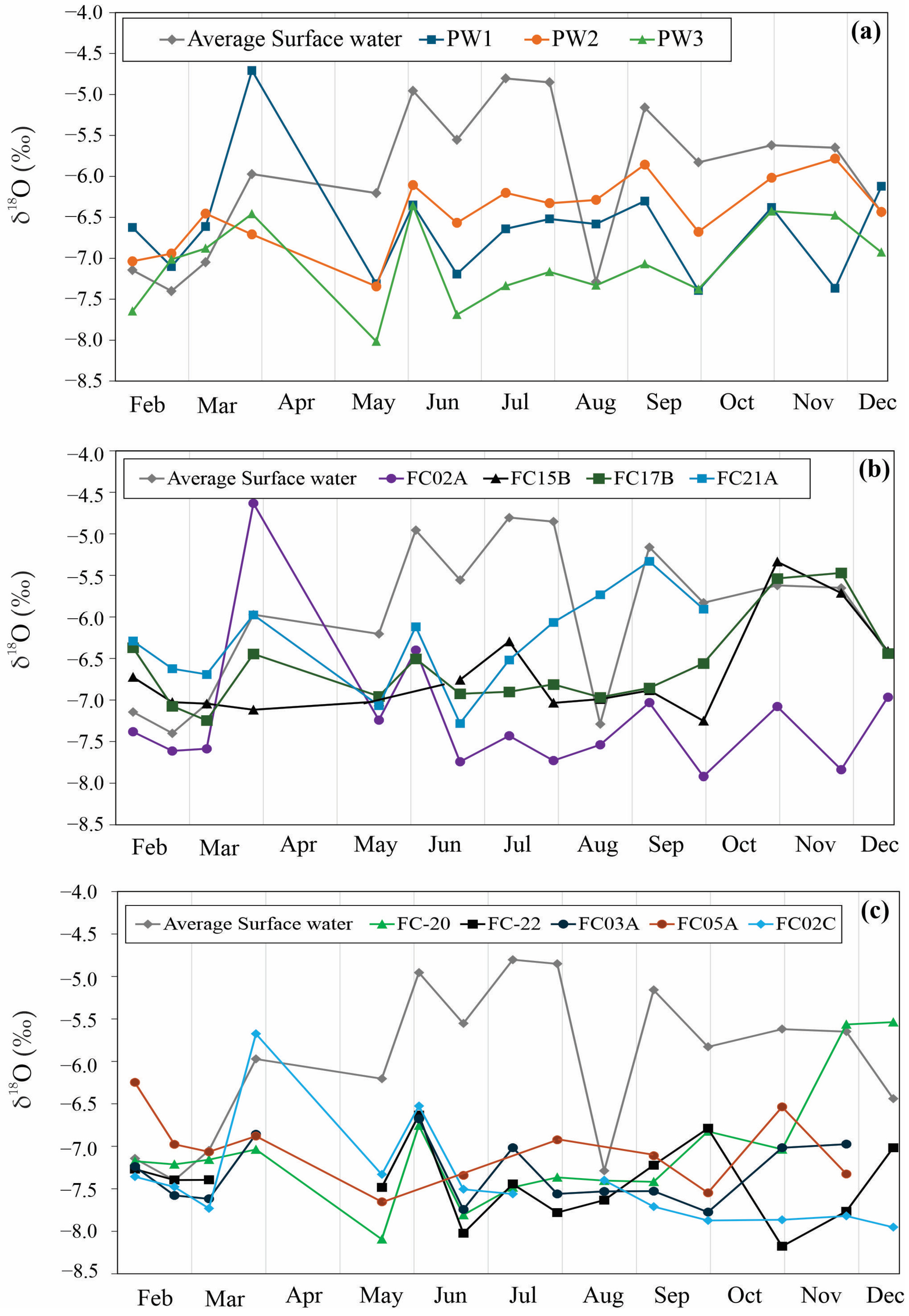
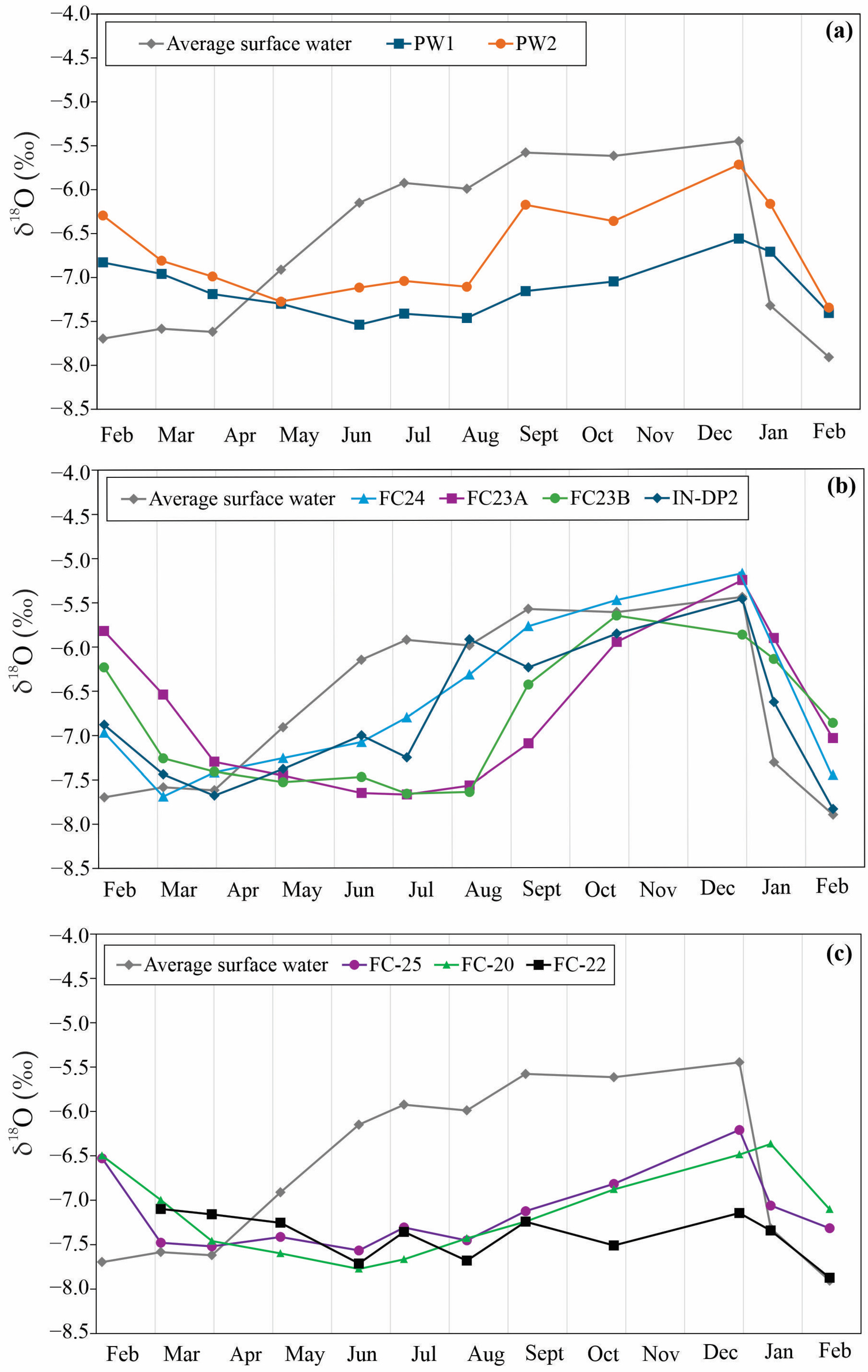
From February to December 2012, 16 sampling rounds were conducted roughly biweekly. During this period, water from all three municipal production wells was sampled (PW1, PW2 and PW3). Surface water samples were collected from creek locations closest to the production wells and from Acton Lake, a reservoir that discharges to Four Mile Creek about 4 km north of PW1. Groundwater samples were taken from four monitoring wells assumed to be affected by induced infiltration and five monitoring wells assumed to be unaffected by induced infiltration. Between February 2021 and March 2022, sampling was conducted 12 times, approximately monthly. Due to resource limitations, only the two radial production wells were sampled, PW1 and PW2. Surface water was sampled from two creek locations closest to PW1 and PW2. Groundwater was sampled from five monitoring wells assumed to be affected by induced infiltration and three other monitoring wells assumed to not be affected by induced infiltration.

Before taking a water sample at each location, the sampling equipment was rinsed with deionized water, followed by a rinse with water from the sampling location. Water from the municipal production wells was sampled by first allowing the tap to run for about 10 min. This was done to be certain that the sample being collected was representative of pumped water and not water that was sitting in the pipes. For groundwater samples, the monitoring wells and the drive point piezometers were purged before sample collection. The purging was done by bailing out three well volumes before collecting a sample. All the water samples were collected in plastic Whirl Pak^® bags, brought to a laboratory at Miami University and filtered using 0.45 µm filter paper into 30 mL HDPE bottles. The bottles were shipped to the University of Kentucky stable isotope laboratory for analysis. All water samples were analyzed using the Los Gatos Research (LGR) Liquid Water Isotope Analyzer. The isotope ratios were reported using the Vienna Standard Mean Ocean Water (VSMOW) δ-notation (‰). Both oxygen and hydrogen ratios were normalized using the SLAP (Standard Light Antarctic Precipitation) scale with two certified standards: the USGA49 Antarctic Ice Core water (δ²H VSMOW-SLAP = −394.70‰, δ¹⁸O VSMOW-SLAP = −50.55‰) and the USGS Lake Kyoga water (δ²H VSMOW-SLAP = 32.80‰, δ¹⁸O VSMOW-SLAP = 4.95‰). Precision and accuracy were checked using a blind standard USGS45 Biscayne Aquifer Drinking Water (δ²H VSMOW-SLAP = −10.3‰, δ¹⁸O VSMOW-SLAP = −2.24‰).

2.2. Estimating Induced Infiltration

To quantify the amount of induced infiltration in water from the production wells, we used a simple two-component mixing approach using the time-averaged isotopic values at each sampling point (Equation (1)). Time averaged isotopic values of surface water and groundwater not affected by induced infiltration were used as the endmembers.

$$\% Induced Infiltration=100\times {\displaystyle \frac{I{V}_{PW}-I{V}_{GW}}{I{V}_{SW}-I{V}_{GW}}}$$

(1)

where IV_PW, IV_GW and IV_SW are the isotopic values, respectively, of the production well water, the groundwater not influenced by induced infiltration, and surface water. The sampling periods of 2012 and 2021/2022 were evaluated separately.

We hypothesized that a variable portion of water being produced by municipal wells set near surface water bodies came from induced infiltration, and the proportion could be estimated using δ¹⁸O and δ²H signatures of the different water sources. Because most of the groundwater recharge occurs in winter, our assumption was that the isotopic composition of groundwater that is not influenced by induced infiltration would have lower values of both δ¹⁸O and δ²H reflecting the colder winter temperatures. On the other hand, we expected surface water to have isotopic compositions with a wide range of values, as it is a mixture of baseflow from groundwater and overland flow from all the seasons.

3. Results

The results presented include individual sample results along with the means and variances of δ¹⁸O and δ²H over time for each sampling location. The sampling locations represent four groups: (1) surface water from Four Mile Creek, (2) groundwater that is affected by induced infiltration (groundwater from monitoring wells located on the flow path between the production wells and Four Mile Creek), (3) groundwater that is not affected by induced infiltration and (4) production well water comprising a combination of waters that originally belonged to other groups.

3.1. Deuterium vs. Oxygen-18 Plots for Individual Samples

Plots of δ²H vs. δ¹⁸O for individual samples were made for (1) surface water, (2) groundwater that is affected by induced infiltration and (3) groundwater that is not affected by induced infiltration (Figure 5). We were interested in how the plots compared to the LMWL for Dayton Ohio, and whether there were any significant differences between the groups. The fitted line for surface water was δ²H = 5.42 × δ¹⁸O − 6.72 (Figure 5a). The fitted line for groundwater affected by induced infiltration was δ²H = 4.86 × δ¹⁸O − 10.3 (Figure 5b). The fitted line for groundwater not affected by induced infiltration was δ²H = 4.40 × δ¹⁸O − 14.0 (Figure 5c). The three groups’ regression slopes and intercepts were compared using indicator–variable regression analysis, as described by [28]. The slope for surface water (5.42) was significantly higher (p = 0.007) than the slope for groundwater not influenced by the induced infiltration of surface water (4.40). There was no significant difference between the slopes for groundwater affected by induced infiltration (4.86) and groundwater not affected by induced infiltration (4.40). Additionally, there was no significant difference between the slopes for surface water (5.42) and groundwater from monitoring wells affected by induced infiltration (4.86).

3.2. Changes in δ²H vs. δ¹⁸O Throughout the Study Periods

Figure 6 and Figure 7 represent the δ¹⁸O values throughout the 2012 and 2021/2022 study periods, respectively. δ²H values are not shown as the temporal patterns for δ²H and δ¹⁸O were similar. In 2012, as expected, surface water δ¹⁸O and δ²H values were generally lower in the months of February and March, and higher between April and mid-December (Figure 6a), with the exception of August. For groundwater that we believed to be affected by induced infiltration, the δ¹⁸O and δ²H values were generally lower in the months of February through August, and higher from September to December (Figure 6b), possibly indicating a time lag of about four months compared to surface water. For groundwater that we believed to be unaffected by induced infiltration, the δ¹⁸O and δ²H values were generally lower than surface water in all the months (Figure 6c).

Surface water during the 2021/2022 study period had lower isotopic values from January to April, and higher values from June through December (Figure 7a). There were similar patterns for groundwater that we believed to be affected by induced infiltration (Figure 7b). The wells closest to Four Mile Creek (FC24 and IN-DP2) had increasing values beginning about a month later than surface water. Wells much farther from the creek (FC23A and FC23B) lagged behind surface water by around four months. As in 2012, the isotopic values for groundwater not affected by induced infiltration stayed relatively constant and generally lower than surface water throughout the year.

3.3. Surface Water Time-Averaged Values

Water from the 2012 surface water sampling sites had time-averaged δ¹⁸O values ranging from −6.03‰ to −5.41‰, with an overall mean of −5.86‰ (Figure 8a, Table S2). The time-averaged δ²H values ranged from −39.32‰ to −31.52‰ with an overall mean of −37.13‰ (Figure 8a, Table S2). For the 2021/2022 samples, time-averaged δ¹⁸O and δ²H values were lower (Figure 8b, Table S6) and less variable. The δ¹⁸O values ranged from −7.93‰ to −5.32‰ with an overall mean of −6.65‰. The δ²H mean values for surface water ranged from −42.83‰ to −42.85‰ with a mean of −42.84‰.

The 2012 δ¹⁸O standard deviation for surface water for individual sampling locations ranged from 0.81‰ to 1.24‰ (Figure 9a), and δ²H standard deviation ranged from 4.25‰ to 6.86‰ (Figure 9b). In 2021/2022, the standard deviations were much lower, ranging from only 0.92‰ to 0.9‰ for δ¹⁸O (Figure 9c) and 4.70‰ to 5.00‰ for δ²H (Figure 9d). In general, surface water had both the highest mean and standard deviation values of both δ¹⁸O and δ²H.

3.4. Groundwater Affected by Induced Infiltration

As expected, for both sampling periods, the δ²H and δ¹⁸O mean and standard deviation isotopic values for groundwater believed to be affected by induced infiltration were generally intermediate between surface water and groundwater that was not affected by induced infiltration. In 2012, the monitoring wells identified as having groundwater affected by induced infiltration included FC02A, FC15B, FC17B and FC21A. The time-averaged δ¹⁸O values ranged from −7.21‰ to −6.20‰ with an overall mean of −6.74‰ (Figure 8a, Table S4). The time-averaged δ²H values ranged from −46.22‰ to −39.90‰ with an overall mean of −42.91‰ (Figure 6a, Table S4).

In 2021/2022, the monitoring wells identified as having groundwater affected by induced infiltration included FC23A, FC23B and FC24, as well as the creek drive-point piezometers IN-DP1 and IN-DP2. The time-averaged δ¹⁸O values ranged from −6.98‰ to −6.68‰, with an overall mean of −6.82‰ (Figure 8b, Table S7). The time-averaged δ²H values ranged from −44.45‰ to −42.38‰ with an overall mean of −43.76‰ (Figure 6b, Table S7). The monitoring wells FC23A, FC23B and FC24 and drive point IN-DP2 are on the flow path between Four Mile Creek and PW1, and water from these monitoring wells showed intermediate isotopic compositions. The isotope values of these monitoring wells could be ranked in order of their proximity to Four Mile Creek, with the exception of the drive-point piezometer IN-DP2 (Figure 10). FC24 is the closest monitoring well to Four Mile Creek and had the highest values out of all the monitoring wells at this site, whereas FC23A is the farthest from the stream and is closer to the production well, and had lower values.

In 2012, the δ¹⁸O standard deviation ranged from 0.29‰ to 0.79‰ for sampling locations (Figure 9a), and the δ²H standard deviation ranged from 1.72‰ to 3.32‰ (Figure 9b). In 2021/2022, the δ¹⁸O standard deviation ranged from 0.61‰ to 0.82‰ (Figure 9c), and the δ²H standard deviation ranged from 3.97‰ to 3.30‰ (Figure 9d).

3.5. Groundwater Not Affected by Induced Infiltration

As expected, during both sampling periods, water from wells not affected by induced infiltration had the lowest δ¹⁸O and δ²H time-averaged mean values. In 2012, the monitoring wells identified as having groundwater that was not affected by induced infiltration were FC02C, FC03A, FC05A, FC20 and FC22. The time-averaged δ¹⁸O values ranged from –7.43‰ to −7.05‰ with an overall mean of −7.25‰ (Figure 8a and Figure 9a, Table S3). The time-averaged δ²H values ranged from −47.91‰ to −43.83‰, with an overall mean of −45.89‰ (Figure 8a, Table S3).

In 2021/2022, the monitoring wells identified as having groundwater that was not affected by induced infiltration were FC20, FC22 and FC25. The time-averaged δ¹⁸O values ranged from −7.40‰ to −7.13‰ with an overall mean of −7.22‰ (Figure 8b and Figure 7c, Table S8). The time-averaged δ²H values ranged from −47.00‰ to −45.71‰ with an overall mean of −46.21‰ (Figure 8b, Table S8).

In both periods, the standard deviations of the isotopic values were also relatively low. In 2012, the δ¹⁸O standard deviation ranged from 0.37‰ to 0.69‰ (Figure 9a), and the δ²H standard deviation ranged from 1.09‰ to 3.81‰ (Figure 9b). In 2021/2022, the δ¹⁸O standard deviation ranged from 0.25‰ to 0.45‰ (Figure 9c), and the δ²H standard deviation ranged from 1.48‰ to 2.09‰ (Figure 9d).

3.6. Production Well Water

Production well water during both sampling periods generally had intermediate mean δ¹⁸O and δ²H values, whereas the standard deviations were generally low. The 2012 PW1 δ¹⁸O values ranged from −7.39‰ to −4.71‰, with an overall time-averaged mean of −6.61‰ and standard deviation of 0.65‰ (Figure 8a and Figure 9a, Table S1). The δ²H values ranged from −47.86‰ to −32.01‰, with an overall time-averaged mean of −42.74‰ and a standard deviation of 3.49‰ (Figure 8a and Figure 9b, Table S1). PW2 δ¹⁸O values ranged from −7.34‰ to −5.74‰, with an overall time-averaged mean of −6.45‰ and a standard deviation of 0.43‰ (Figure 8a and Figure 9a, Table S1). The δ²H values ranged from −47.82‰ to −36.29‰, with an overall time-averaged mean of −42.43‰ and a standard deviation of 2.84‰ (Figure 8a and Figure 9b, Table S1). PW3 had the lowest values, for both δ¹⁸O and δ²H. The δ¹⁸O values ranged from −8.02‰ to −6.36‰, an overall time-averaged mean of −7.08‰ and a standard deviation of 0.49‰ (Figure 8a and Figure 9a, Table S1), whereas δ²H values ranged from −47.70‰ to −40.35‰, an overall time-averaged mean of −45.11‰ and a standard deviation of 1.94‰ (Figure 8a and Figure 9b, Table S1). Both the δ²H and δ¹⁸O averages and the standard deviation of PW3 were similar to those of groundwater that was from monitoring wells not influenced by induced infiltration. Of the three production wells, PW2 had the highest δ¹⁸O values. PW1 and PW2 had similar averaged δ²H isotopic values; however, PW1 had a higher standard deviation. The production wells’ δ¹⁸O and δ²H isotopic values fluctuated in a similar pattern to that of surface water (Figure 6a).

The 2021 PW1 δ¹⁸O values ranged from −7.54‰ to −6.15‰, with an overall time-averaged mean of −7.13‰ and standard deviation of 0.30‰ (Figure 8b and Figure 9c, Table S5). The δ²H values ranged from −49.01‰ to −43.52‰, with an overall time-averaged mean of −45.99‰ and standard deviation of 1.52‰ (Figure 8b and Figure 9d, Table S5). PW2 δ¹⁸O values ranged from −7.34‰ to −5.72‰, an overall time-averaged mean of −6.70‰ and a standard deviation of 0.51‰ (Figure 6b and Figure 7c, Table S5). The δ²H values ranged from −46.14‰ to −39.69‰, with an overall time-averaged mean of −43.61‰ and standard deviation of 2.09‰ (Figure 8b and Figure 9d, Table S5). The time-averaged δ¹⁸O value of PW2 was similar to those of most of the surface water values but with a lower standard deviation. In general, the production wells’ δ¹⁸O and δ²H isotopic values were lower from the month of January to May, with constant values from June to mid-August and higher values from September through to December (Figure 7a). The rise in surface water values in April followed by a rise in production well values in September suggests a possible time lag of about five months for the production wells compared to surface water.

3.7. Estimating Induced Infiltration

The δ¹⁸O and δ²H signatures of surface water and groundwater from monitoring wells not affected by induced infiltration provided the end-member isotopic compositions with which we estimated the amount of induced infiltration at each production well. This approach was used by Hunt et al. and Maloszewski et al. [19,30]. For each production well, we picked two endmembers. One endmember represented groundwater from the closest monitoring well not on the flow path between surface water and the production well (i.e., assumed to not be affected by induced infiltration). The other endmember was surface water from Four Mile Creek at the sampling point closest to each production well. Using the time-averaged δ¹⁸O and δ²H values (Figure 11) of the production wells and their respective end members, we used Equation (1) to quantify the fraction of production well water originally emanating from induced infiltration (

Table 1. 2012 and 2021/2022 time-averaged δ¹⁸O (‰) end members.

Production Well	δ18O (‰)	δ2H (‰)	Ground Water	δ18O (‰)	δ2H (‰)	Surface Water	δ 18O (‰)	δ2H (‰)
2012 samples
PW1	−6.62	−42.74	FC 22	−7.43	−47.97	FMC1	−6.00	−39.32
PW2	−6.45	−42.44	FC 20	−7.06	−43.84	FMC2	−6.03	−39.28
PW3	−7.08	−45.11	FC 03	−7.27	−46.40	FMC3	−6.01	−38.41
2021/2022 samples
PW1	−7.13	−45.99	FC 22	−7.40	−46.98	FMC1	−6.63	−42.85
PW2	−6.70	−43.50	FC 20	−7.13	−45.71	FMC2	−6.66	−42.83

). Discharge volumes or pumping rates were not used in calculating the percent of induced infiltration; only the time-averaged isotope values of both δ¹⁸O and δ²H were used.

3.7.1. Production Well 1

In 2012, at PW1, FMC1 was used as a surface-water endmember and FC22 was the groundwater endmember (Table 1). Using δ¹⁸O and δ²H time-averaged values, the estimated percentages of water originating from the induced infiltration of surface water were 57% and 61%, whereas groundwater accounted for 43% and 39%, respectively. In 2021/2022, we used the same endmember sampling points as in 2012. Using δ¹⁸O and δ²H time-averaged mean values, the estimated percentages of induced infiltration of surface water were 35% and 24%, respectively; groundwater accounted for 65% (using δ¹⁸O) and 76% (using δ²H) (

Table 2. Percent induced infiltration.

Production Well	δ18O		δ2H
	% SW	% GW	% SW	% GW
2012 samples
PW1	57	43	61	39
PW2	59	41	31	69
PW3	15	85	16	84
2021/2022 samples
PW1	35	65	24	76
PW2	91	9	77	23

).

3.7.2. Production Well 2

In 2012, at PW2, FMC2 was used as a surface water endmember, and FC20 was the groundwater endmember (Table 1). Using δ¹⁸O and δ²H time-averaged values, the estimated percentages of water originating from the induced infiltration of surface water were 59% and 31%, whereas groundwater accounted for 41% and 69%, respectively. In 2021/2022, we used the same endmembers as in 2012. Using δ¹⁸O and δ²H time-averaged mean values, the percentages of induced infiltration of surface water were 91% and 77%, while groundwater accounted for 9% and 23%, respectively (Table 2).

3.7.3. Production Well 3

PW3 was analyzed only in 2012, and we used FMC3 and FC03 as the endmembers for surface water and groundwater, respectively (Table 1). Using δ¹⁸O and δ²H time-averaged values, the estimated percentages of water originating from the induced infiltration of surface water were 15% and 16%, while groundwater accounted for 85% and 84%, respectively, (Table 2). Of the three production wells, PW3 had the lowest estimates of induced infiltration, while PW2 in 2021 had the highest.

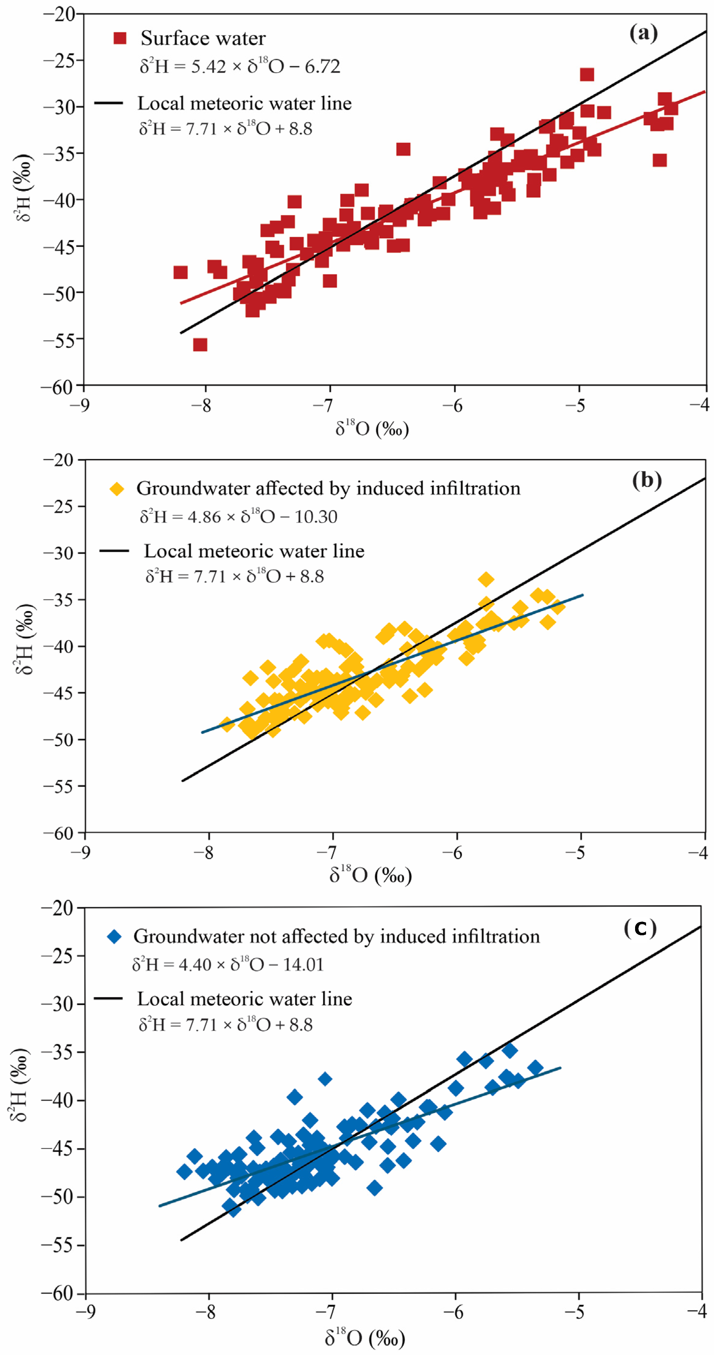
4. Discussion

4.1. Groundwater and Surface Water vs. the LMWL

To understand the amount of evaporation that has occurred and deduce any surface water and groundwater interactions, we compared relationships of δ²H vs. δ¹⁸O for surface water and groundwater to the LMWL for southwest Ohio, as provided by Bedaso and Wu [14] (Figure 5). The slopes of surface water, groundwater affected by induced infiltration and groundwater not affected by induced infiltration were all lower than the LMWL, indicating that all these waters underwent evaporation prior to the sampling of surface water and prior to the recharging of the groundwater. The slopes for the groundwater were lower than the slope for surface water, possibly due to continued kinetic evaporation in the phreatic or unsaturated zone of the aquifer [4,31].

4.2. Surface Water Isotopic Composition

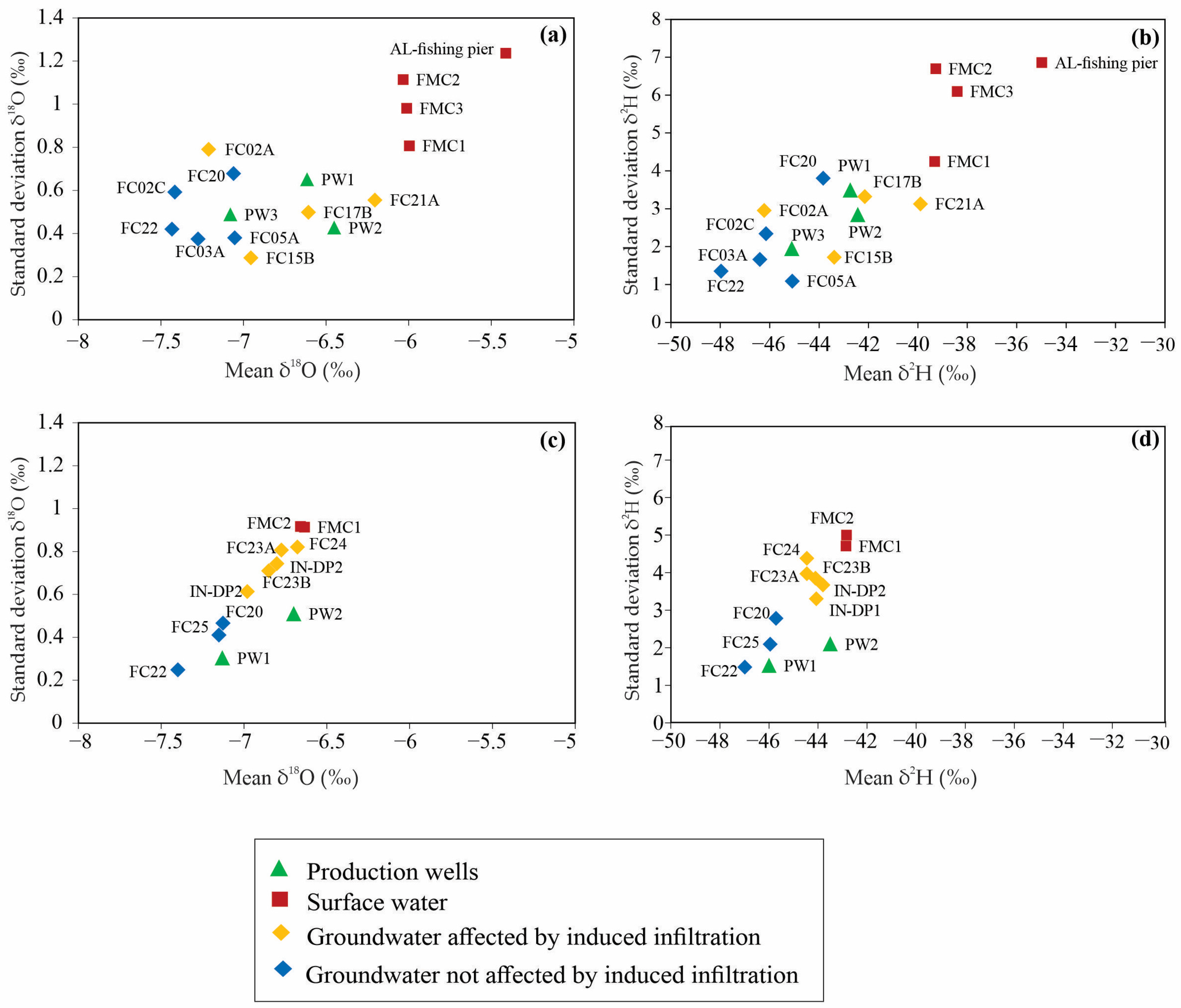
Because both the δ¹⁸O and δ²H values had similar patterns, for this part of the discussion, we will focus on the δ¹⁸O values. As expected, surface water samples had higher average isotopic mean values and standard deviations than did groundwater. Surface water comprises both baseflow (and therefore has an isotopic signature like groundwater) and overland flow from precipitation throughout the year. The result is that in summer, the isotopic values can vary widely depending on how long after a storm event the sampling occurred. Despite the variability, there was a consistent seasonal trend in the isotopic composition of surface water, with lower values between mid-December and March and higher values between April and November during both sampling periods. The lowest δ¹⁸O and δ²H values occurred between the months of February and March, a period dominated by Pacific-source moisture.

4.3. Isotopic Composition of Groundwater Not Affected by Induced Infiltration

For all the samples of groundwater believed to not be affected by induced infiltration, the ranges of δ¹⁸O values throughout the study periods were −8.18‰ to −5.54‰ for 2012 and −7.87‰ to −6.21‰ for 2021/2022 (Tables S3 and S8). As expected, groundwater sampled from monitoring wells that were identified as not influenced by induced infiltration was lowest in both the means over time and the standard deviations of the isotopic values. Unlike surface water and groundwater affected by induced infiltration, there was no seasonal trend in the isotopic composition of groundwater that was not affected by induced infiltration. This is most likely due to the fact that groundwater recharge in southwest Ohio occurs mostly in the winter and early spring, and does not reflect seasonal variability. In the mid-latitudes, winter and early-spring precipitation recharges groundwater more than summer precipitation [29,32] due to the reduced evapotranspiration. While summer precipitation can be very intense, more of it is lost to evapotranspiration due to high temperatures and vegetation growth [33,34]. The average δ¹⁸O values for groundwater were −7.25‰ and −7.22‰ for 2012 and 2021, respectively. The variability that did exist was consistent with the fact that the Arctic precipitation source, while having the lowest average δ¹⁸O value, also has largest variability during the winter [14]. While these were the lowest averages at our site, they were higher than the isotopic composition of the local winter precipitation (Dayton area average of −8.8‰), which could reflect early spring recharge.

4.4. Isotopic Composition of Groundwater Affected by Induced Infiltration

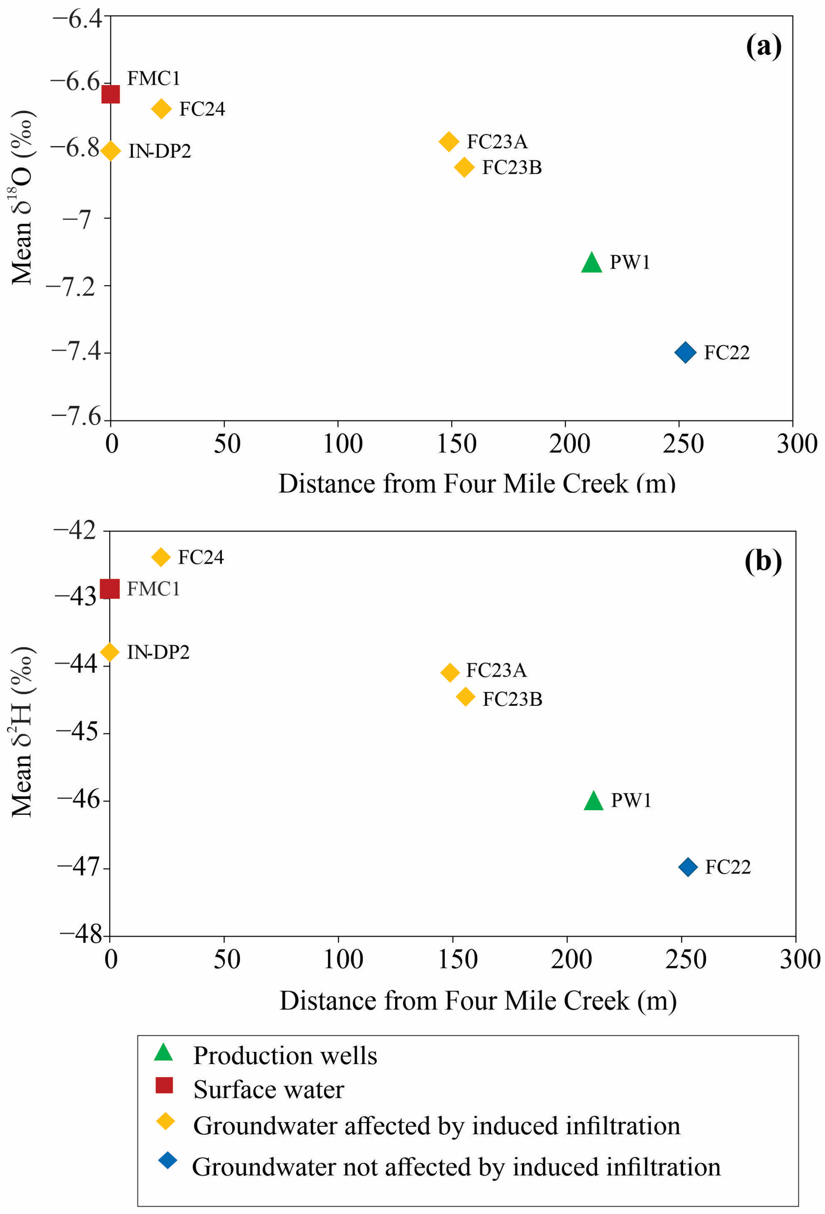
For the monitoring wells on the flow path between the stream and the production wells, the isotopic values decreased with increasing distance from the stream (Figure 10). This suggests that there was more influence from stream water at sampling points closer to the stream. Johnstone et al. [35] found similar results in groundwater in the Great Miami River Basin in southwest Ohio, where groundwater from shallow wells closer to the rivers and streams had higher δ¹⁸O compared to lower values in deeper wells and those farther from the surface water.

4.5. Isotopic Composition of Production Well Water

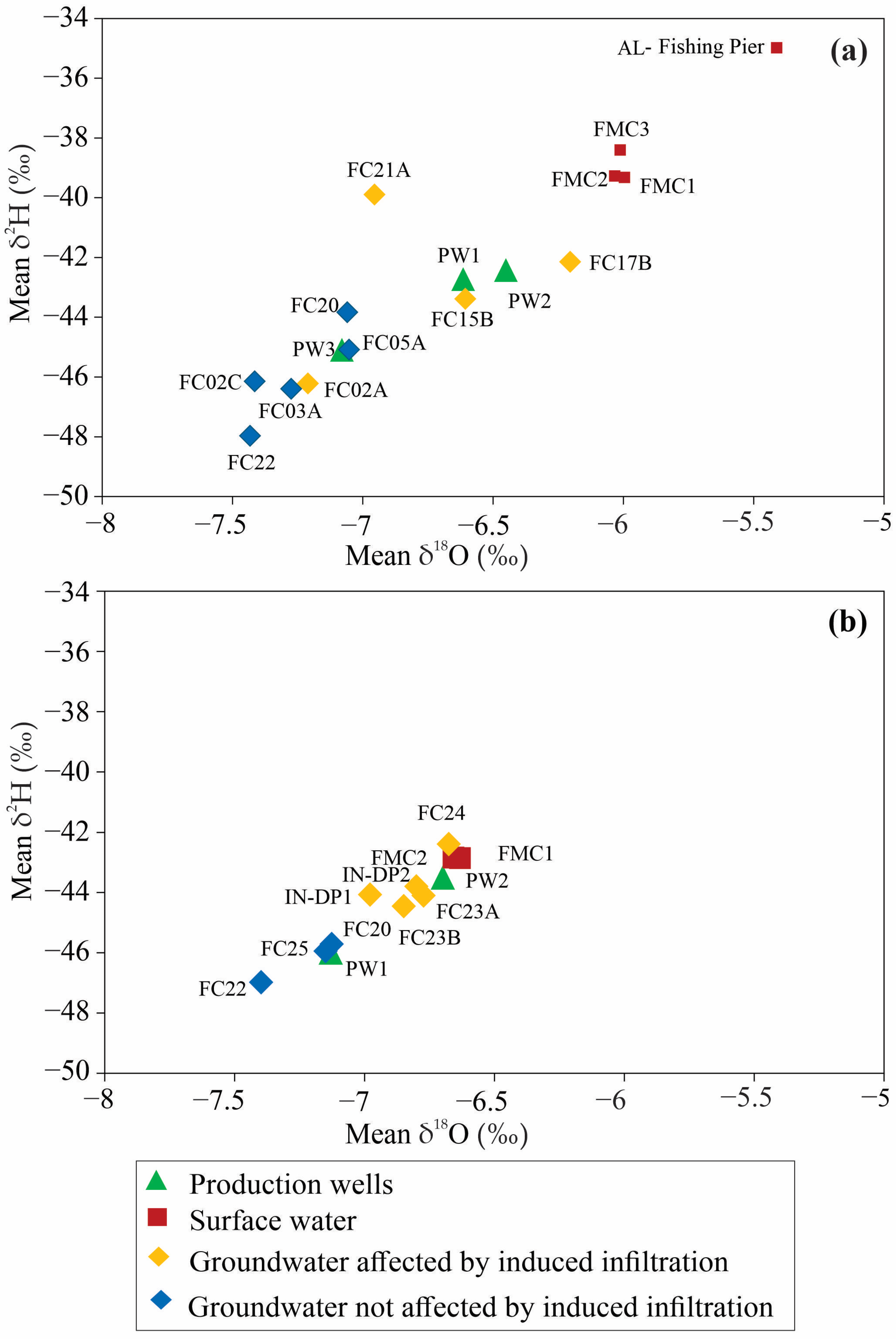
As expected, groundwater from the production wells had mean isotopic values that were intermediate between surface water and groundwater, allowing an estimation of the contribution of induced infiltration. Our hypothesis was that the mean values were intermediate due to mixing. We initially expected that the standard deviations of δ¹⁸O and δ²H values in production-well water would also be intermediate, but interestingly, production-well water had relatively low standard deviations of both δ¹⁸O and δ²H values. The low variability is probably due to the fact that the production wells pull in water from areas that include a wide array of long and short flow paths that began both widely spread in the groundwater system and in reaches of Four Mile Creek. The water collected in the production wells at any time is a mix of water that began as precipitation any time from very recently to several years ago. Because this water is thoroughly mixed, it represents a long-term average, and therefore does not vary much over time.

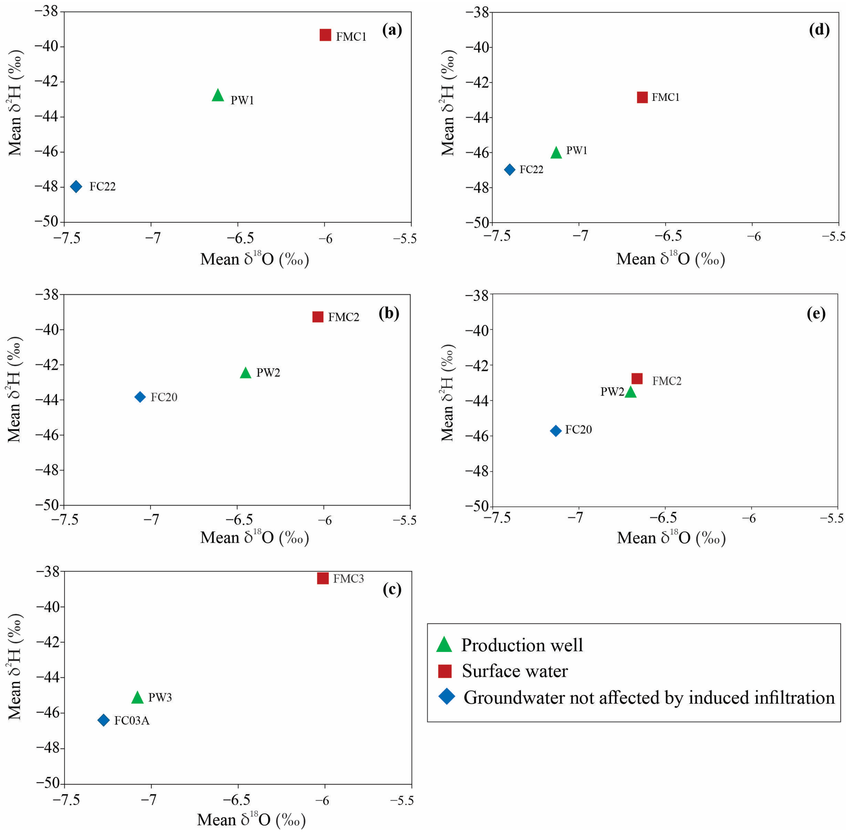
PW1 is about 200 m from Four Mile Creek, and yet the average δ¹⁸O and δ²H isotope values of groundwater at PW1 were similar to those of surface water, suggesting that most of the water pumped was originally derived from the induced infiltration of water from Four Mile Creek. These results are consistent with the fact that the hydraulic gradients between the creek and underlying groundwater system were strongly downward throughout both study periods. The head below the creek and gradients clearly responded to the pumping at PW1. The downward gradients were stronger when the pump was on and not as strong when the pump was off, but still downward. We estimated a greater contribution of induced infiltration at PW1 in 2012 than in 2021/2022 (57% versus 35% using δ¹⁸O and 61% versus 24% using δ²H).

Our estimations of induced infiltration at PW2 are higher than for the other two wells. PW2 is only 25 m from Four Mile Creek. Using δ¹⁸O at PW2, we estimated that induced infiltration from Four Mile Creek made up 59% of produced water in 2012 and 91% in 2021/2022. Using δ²H, we estimated that induced infiltration accounted for 31% of the produced water in 2012 and 77% in 2021/2022. In the vicinity of PW2, there is a clay layer with a top elevation between about 232.6 m to 234.1 m above msl, and with a bottom elevation of around 231 m. Four Mile Creek at PW2 is at an elevation of about 233.4 m, with the creek bed at approximately 232.5 m above msl. We do not know the north-to-south extent of this confining bed, but we do know that it extends from at least 73 m west of Four Mile Creek to 34 m east of Four Mile Creek. When PW2 is pumping, the hydraulic head below the creek bed drops to about 1.7 m below the elevation of the creek bed and about 0.8 m below the bottom of the clay layer. This means that when PW2 is pumping, the creek is disconnected from the groundwater system under the creek at PW2. Despite this lack of hydraulic connection, the isotopic data indicate that much of the water in PW2 comes from induced infiltration. We hypothesize that this water is mostly entering the groundwater system upstream and/or downstream of PW2, where the clay layer is not present. More stratigraphic investigations upstream and downstream of PW2 would be required to test this hypothesis.

PW3 was only investigated in 2012. It is the farthest of the production wells from Four Mile Creek (about 230 m), and is a conventional vertical well as opposed to a radial collector well. It had the lowest pumping rate of the three wells, pumping on average about 0.6 m³/min compared to about 2 m³/min at PW1 and PW2. It is therefore not surprising that the isotopic values showed the least contribution from induced infiltration. Using δ¹⁸O and δ²H values, we estimated that 15% and 16%, respectively, of water pumped by PW3 originally came from induced infiltration. Hydraulic gradients between the creek and underlying groundwater near PW3 were consistently downward, as at PW1; however, the magnitude of the gradients was substantially less (about 0.35 compared to 0.55), and neither the head below the creek nor the gradients responded to the pump at PW3 being turned on and off.

Comparing the two radial collector wells PW1 and PW2, our results indicate that the amount of induced infiltration from surface water varies and depends on the distance of a wells’ horizontal arms from the stream. PW2 is closer to the stream than PW1, and hence this could explain why we observed more water originating from the stream at PW2 than PW1. Comparing all three wells, PW3 had the lowest percentage of induced infiltration. In terms of well structure, PW3 is a vertical conventional well and tends to draw smaller volumes of water compared to the collector wells. In addition, PW2 and PW1 have higher pumping rates compared to PW3. Overall, the percentages of induced infiltration in all the three wells varied as a result of different well pumping rates, durations of pumping, well structures (radial or vertical conventional well) and the horizontal distance between the production well and the stream.

4.6. Sampling Period Comparison: 2012 vs. 2021/2022

During both 2012 and 2021, groundwater had lower δ¹⁸O and δ²H values than surface water. While the δ¹⁸O and δ²H patterns for both sampling periods were similar, there were differences in the isotopic values between the two periods. Water sampled in 2012 had a greater range of isotopic values, and those values were greater on average than those in water sampled in 2021 (Figure 8). One possible explanation is that warmer temperatures and lower humidity caused precipitation and surface water to have higher values in 2012 than in 2021. According to the National Weather Service [36], some parts of Ohio, Indiana and Michigan had record high temperatures in 2012. The average annual temperature of this region in 2012 was 12.2 °C, a record-breaking high [37] compared to an annual average of 11.8 °C in 2021. The high temperatures in 2012 were mostly concentrated in the winter and spring. In addition, there was low humidity in 2012 due to a drought in the fall and spring [36].

Our estimates of the contributions of induced infiltration at PW1 and PW2 were very different in the two study periods. The estimate of the contribution of induced infiltration at PW1 was almost 30% greater in 2012 compared to 2021/2022, and this was mostly due to a drop in the average δ¹⁸O and δ²H values (Figure 11). This is likely the result of higher pumping rates for PW1 in 2012 than in 2021/2022 (Supplementary Figure S1). The PW1 pumping rates in 2012 varied, but there were long periods of pumping with rates that averaged around 1.3 × 10⁶ m³/y, while in 2021/2022 the pumping rates averaged around 9.0 × 10⁵ m³/y, also about 30% lower than in 2012. For PW2, we estimated a much higher percent induced infiltration during the 2021/2022 sampling period than in 2012. Again, part of the difference may be explained by higher pumping rates in much of 2021/2022 (1.5 × 10⁶ m³/y) than in 2012 (7 × 10⁵ m³/y). Also, the pump at PW2 was on for most of the sampling period in 2021/2022. However, unlike at PW1, the δ¹⁸O and δ²H values at PW2 changed little between the two periods. Instead, the major difference was a drop in the δ¹⁸O and δ²H values of Four Mile Creek water in 2021/2022 compared to 2012. With this drop, water from PW2 became more isotopically similar to surface water. The reason for the change in surface water isotopic values is unknown, but the differences between the two periods do indicate how sensitive the results are to the variability inherent in the surface water δ ¹⁸O and δ²H values.

4.7. Comparison of Results Using δ¹⁸O vs. δ²H

Estimations of the contributions from induced infiltration at the production wells varied depending on whether we used the δ¹⁸O values or the δ²H values. For PW1 and PW3 in 2012, the differences were minimal—about 3.6% for PW1 and <1% for PW3. At PW3, however, the results differed by almost 29%. In 2021/2022, the results differed by 11.0% and 14.6% for PW1 and PW2, respectively. Reasons for the discrepancies are unknown, and it is not clear whether the δ¹⁸O values or the δ²H values are more reliable indicators of induced infiltration. The discrepancies indicate that caution should be used in interpreting the results, as they give some indication of the uncertainty inherent in the method. The rather large discrepancy for PW2 in 2012 indicates that the method should only be used semi-quantitatively.

5. Conclusions

This study explored the use of stable isotopic signatures of groundwater and surface water to estimate the contribution of induced infiltration in municipal production well water. Such an estimation is important in order to understand the risks associated with surface water contaminants entering a groundwater system and with damaging groundwater-dependent riparian ecosystems. The method was applied to a municipal well field in Oxford, Ohio that comprised three production wells in a sand-and-gravel glacial outwash aquifer adjacent to Four Mile Creek. The wells varied by distance to the creek and pumping rates.

The results indicate that the two radial collectors, PW1 and PW2, which pump an average of 1.3 × 10⁶ m³/y and 9 × 10⁵ m³/y, respectively, showed a greater contribution of induced infiltration, with the closer of the two to the streams comprising the most water from induced infiltration. PW3 was a conventional vertical well with a much lower average pumping rate (7 × 10⁵ m³/y) and was the farthest from the stream. The δ¹⁸O and δ²H values indicate that induced infiltration was as much as 91% of the water produced from PW2 in 2021/2022 and as little as 15% of the water produced from PW3 in 2012. These results are consistent with hydraulic-gradient data indicating the degree of hydraulic connection between the pumping wells and the stream. The results are also consistent with δ¹⁸O and δ²H values in water from monitoring wells that were along the flow paths from the stream to the production wells. For those monitoring wells that were assumed to be affected by induced infiltration, the δ¹⁸O and δ²H values were intermediate between other groundwater and stream water.

Differences in isotopic values and estimates of induced infiltration between sampling periods and between using δ¹⁸O and δ²H values indicate that there was a substantial amount of uncertainty associated with the method. The discrepancies between sampling periods may be explained by changing weather conditions and pumping rates. However, the method was quite dependent on determining the average δ¹⁸O and δ²H values of surface water, which show substantial temporal and spatial variability. Because groundwater is generally highly susceptible to contamination, particularly from surface water infiltration, knowing the proportions of surface water in the production wells is important for sustainable water management. The techniques employed in this study can be utilized to understand induced bank infiltration. These results can also be useful to regulatory agencies in charge of protecting streams. Our results demonstrate that stable isotopes of water provide a reliable method of quantifying induced infiltration in alluvial aquifers and can potentially provide high-quality results. The cost of water sample collection and the analysis of isotopes is relatively low (in the USA), and thus makes the method easier to use under budget constraints.