Article

Assessment of Climate Change Impacts on Hydrology Using an Integrated Water Quality Index

1
Department of Civil and Environmental Engineering, Myongji University, Yongin 17058, Republic of Korea
2
Institute for Construction & Environment Engineering, Myongji University, Yongin 17058, Republic of Korea
3
Division of Watershed and Total Load Management Research, National Institute of Environmental Research, Incheon 22689, Republic of Korea
*
Author to whom correspondence should be addressed.
Hydrology 2024, 11(11), 178; https://doi.org/10.3390/hydrology11110178
Submission received: 28 August 2024 / Revised: 12 October 2024 / Accepted: 21 October 2024 / Published: 24 October 2024
(This article belongs to the Section Hydrology–Climate Interactions)

Abstract

Traditional Water Quality Indices (WQIs) often fail to capture the significant impact of flow velocity on water quality, especially under varying hydrological conditions. In this study, an Integrated Water Quality Index (IWQI) was developed by combining water quality parameters and flow rate, providing a more comprehensive assessment under various flow conditions. Compared to traditional indices, the IWQI showed slightly lower correlations in individual parameter performance, but it performed well in evaluating water quality changes associated with flow variations. Parameters such as Total Phosphorus (TP), Total Coliforms (TC), and Fecal Coliforms (FC), which are prevalent pollutants in the Cheongmi River, significantly influenced IWQI scores. River water quality was evaluated using input data simulated under a climate change scenario. When precipitation was abundant, the IWQI score remained relatively stable even with reduced flow rates. However, during periods of insufficient rainfall, water quality deteriorated sharply. While general water quality parameters exhibited approximately a 10% change as flow decreased, TC and FC showed rapid deterioration, with change rates ranging from 20% to 60%. These findings underscore the importance of managing TC and FC, particularly when insufficient rainfall is predicted, as they are major sources of pollution.

1. Introduction

Water Quality Indices (WQIs) were developed to simplify and logically summarize complex water quality information, effectively communicating water quality conditions [1]. These indices provide scientific assessments of water quality using simple ratings and scores that are easy for non-experts to understand. Additionally, they are useful for assessing water quality status by comparing trends and spatial and temporal changes [2]. Generally, WQIs are developed based on expert opinions and watershed characteristics, with important water quality parameters selected and calculated as dimensionless sub-indices. The final water quality index is calculated by assigning weights to each parameter and combining these sub-indices [3]. However, although WQIs are useful for evaluating river water quality comprehensively, they often do not account for flow rate, which closely impacts water quality. Therefore, it is necessary to consider both flow rate and water quality in the context of pollutant dispersion and climate change.
By predicting the WQIs, the importance of various parameters is determined to assign appropriate weights, allowing for accurate prediction of groundwater quality based on the WQI, surface water characteristics, and land and soil properties. This predictive approach minimizes the need for extensive data collection and analysis, enabling real-time water quality assessments. Research that applies various methodologies, such as machine learning, is being actively conducted to provide timely and reliable water quality information [4,5,6].
A review of commonly used water quality indices reveals differences in parameter selection and application. The Canadian Council of Ministers of the Environment Water Quality Index (CCME WQI) allows for flexible parameter selection depending on the specific water quality assessment objective. In contrast, the National Sanitation Foundation Water Quality Index (NSFWQI), Oregon Water Quality Index (OWQI), and Real-Time Water Quality Index (RTWQI) primarily use predefined parameters set by the organizations that developed them. However, in some studies, the parameters are modified due to missing or unobserved data and based on the specific objectives of the research. The CCME WQI generally uses the following parameters: Potential of Hydrogen (pH), Biochemical Oxygen Demand (BOD), Suspended Solids (SS), Dissolved Oxygen (DO), Total Phosphorus (TP), Total Coliforms (TC), and Fecal Coliforms (FC) [7]. The NSFWQI includes DO, Fecal Coliforms, pH, BOD, temperature change, total phosphates, nitrates, turbidity, and total solids [8]. The parameters used in the OWQI are temperature, DO, BOD, pH, ammonia, nitrate nitrogen, total phosphorus, total solids, and fecal coliform. In the RTWQI, the parameters include DO, pH, water temperature, Electrical Conductivity (EC), Total Organic Carbon (TOC), Total Nitrogen (TN), and TP [9,10]. These indices primarily focus on water quality parameters alone.
Additionally, water quality indicesdeveloped by various countries and organizations often yield different results due to methodologicalvariations, which depend on the parameters used and the calculation methodsapplied. For example, Prati’s index estimates lower scores compared to Bhargava’s WQI and the NSFWQI, while the OWQI and CCME WQI exhibit smaller changes in index scores in response to water quality variations [11]. Ref. [12] used the NSFWQI and OWQI to evaluate spatiotemporal changes in the Talar River’s water quality, finding higher scores for the NSFWQI compared to the OWQI, which showed minimal change over time. Ref. [13] compared the NSFWQI and WAWQI to assess water quality in the Kaani and Kpean rivers, noting that despite similar observations, the WAWQI rated them as excellent while the NSFWQI rated them as moderate. Ref. [14] compared multiple indicators and found significant inconsistencies in water quality assessments within the same watershed. These discrepancies highlight the need for indices that consider watershed characteristics.
Recent climate change has increased the variability and the intensity of annual precipitation, resulting in more frequent and severe floods and droughts [15]. Rivers in Korea, which experience large seasonal flow rate fluctuations, are managed through infrastructure such as dams and weirs, which take geographical and climatic conditions into account for flood control and water resource management [16,17]. However, these structures can alter the river environment, and flow rate control downstream of dams affects river hydrology [18]. In addition, in preparation for climate change, it serves as a factor in altering hydrological characteristics by enhancing the storage capacity of large-scale multi-purpose dams and constructingmultiple weirs in river channels to increase the water storage capacity [19]. In addition, discharge from dams causes water from reservoirs to flow into rivers, changing water quality and causing further changes through this water cycle. The correlation analysis (Pearson) indicates that flow variability is highly correlated with various water quality parameters, such as SS and turbidity [20]. An analysis of the relationship between flow rate and water quality variables in the Nakdong River revealed significant nonlinear variability [21]. In tributaries with lower flow rates compared to the mainstream, pollution from sewage, stormwater runoff, and livestock waste continues, necessitating comprehensive water environment assessments that consider both flow rate and water quality [22]. Understanding the hydrological cycle and water quality changes caused by climate change is crucial [23,24]. River-type reservoirs, such as Paldang Lake, located at the confluence of rivers, require intensive management due to the accumulation of pollutants and elevated pollutant concentrations resulting from river inflows [25,26]. By applying climate change scenarios (RCPs), the outflow of sediments and non-point pollutants increased due to the rise in river discharge [24]. Additionally, under the climate change scenarios (SSPs), reservoir water quality showed significant variability depending on the reservoir volume [27]. To manage river water quality effectively from a climate change perspective, a comprehensive assessment considering flow rate variability is necessary.
The traditional WQIs provide comprehensive information about water quality, but they do not account for flow rate, which significantly impacts water quality. These limitations reduce their effectiveness in assessing contaminant dispersion, particularly under diverse hydrological conditions resulting from climate change.
In this study, we develop an Integrated Water Quality Index (IWQI) that selects water quality parameters based on flow rate and watershed characteristics to evaluate river water quality comprehensively, considering hydrological factors. We perform Factor Analysis (FA) to recalculate the weights to better reflect the characteristics of the watershed. Additionally, we aim to assess the IWQI by utilizing input variables predicted through climate change scenario simulations using both physics-based and data-driven models. Our goal is to provide a comprehensive assessment tool for watershed-based water quality management under a wide range of climatic conditions.

2. Materials and Methods

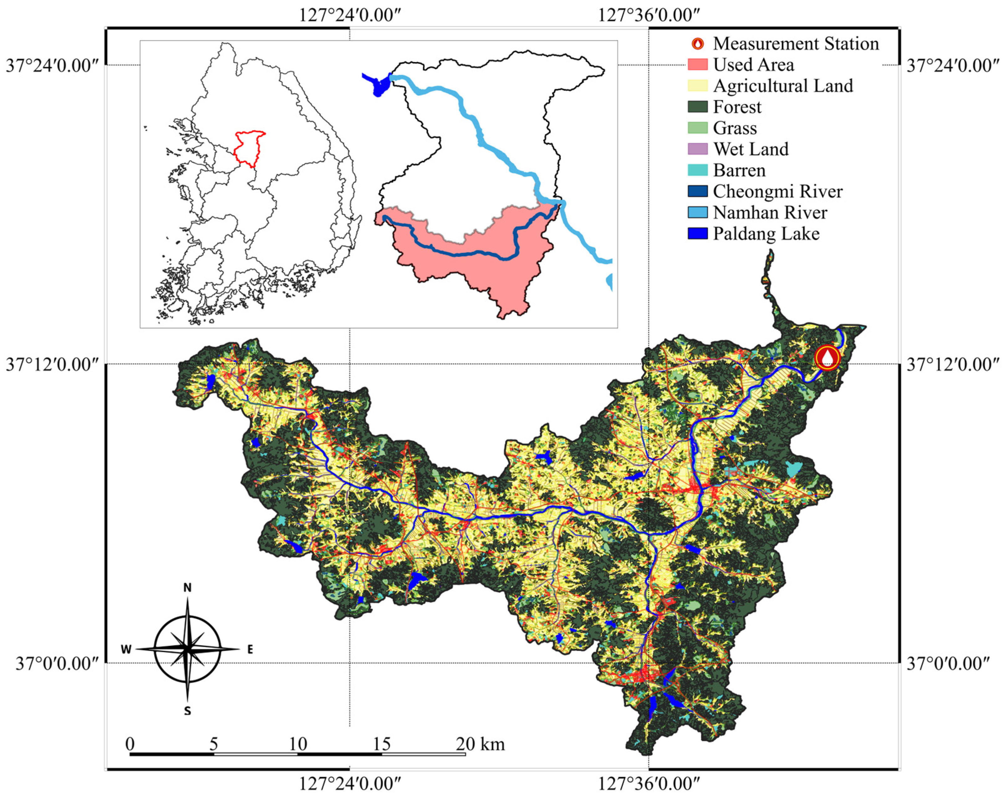
2.1. Study Watershed

Paldang Lake is the largest single water source in Korea, supplying water to 26 million people, half of the country’s population. Therefore, maintaining water quality and the health of aquatic ecosystems is crucial [28]. Paldang Lake is a river-type lake characterized by a short residence time and shallow water depth, and it is highly influenced by pollutants and rainfall due to its large watershed area [29]. Paldang Dam has a limited flood control capacity and shallow water depth due to high inflow and outflow, resulting in complex physical characteristics [30,31]. Water quality fluctuations in Paldang Lake are influenced by climatic, natural, and hydrological factors, necessitating the management of water quality variability, pollution sources, and inflow streams to control problems such as eutrophication and green algae [32]. The Namhan River, which flow rates into Paldang Lake, has a relatively high pollution load, significantly affecting the lake’s water quality [33]. Additionally, the water pollution problem in the Namhan River during the spring dry season complicates the management of Paldang Lake’s water quality [34].
Since the water quality of a river is fundamentally determined by the amount and type of pollutants flowing into it, identifying and controllingpollutants entering the mainstream is critical for water pollution management [33]. The WQI score of the Namhan River decreases downstream mainly due to the inflow of highly polluted tributaries such as the Bokha River, Yanghwa River, and Cheongmi River [34]. Designated as a research area by the International Hydrological Program (IHP), Cheongmi River possesses a rich dataset of long-term hydrological and geomorphological data. Additionally, the BOD concentration is higher at low flow rates, and the TP concentration is higher at high flow rates, indicating the greater influence of point and non-point pollution sources, respectively [35]. Therefore, we conducted a study on the Cheongmi River watershed, which was selected as a priority management tributary due to its high pollution levels and ease of securing data (Figure 1).
As of 2021, the water use status in the middle watershed of the lower Namhan River, which serves as the pilot watershed for the calculation of the IWQI, is as follows: total water use is 560,416.8 thousand m3/year, with 110,683.3 thousand m3/year for residential water (19.8%), 57,493.2 thousand m3/year for industrial water (10.3%), and 392,240.3 thousand m3/year for agricultural water (70.0%). This demonstrates the characteristics of rural areas with high agricultural water use. The impervious area ratio is 9.5%, and according to the research results of the Impervious Cover Model (ICM) in the United States, the watershed condition is rated as good. In addition, the Cheongmi River watershed is characterized by a large proportion of rural areas and forests, with land use distributed as follows: urban area: 4.7%, agricultural land: 40.4%, forest: 40.6%, grass: 9.0%, wet land: 1.8%, barren: 2.1%, and water bodies: 1.5%.
To assess the water quality of the Cheongmi River, we utilized data collected from a single monitoring point located in the lower part of the watershed, where both water quality and flow rate are observed. The coordinates of the observation station are x = 127.7191, y = 37.2022. The dataset spans from 2017 to 2021 and includes 25 parameters, categorized into physical, chemical, biological, organic pollutants, toxic substances, and heavy metals. The physical parameters include water temperature and SS. The chemical parameters comprise DO, BOD, COD, TOC, TN, ammonia nitrogen, nitrate nitrogen, total dissolved nitrogen, TP, phosphate phosphorus, dissolved total phosphorus, pH, and electrical conductivity. Organic pollutants include chlorophyll-a, phenols, and anionic surfactants. The biological parameters are total coliform count and fecal coliform count. Toxic and heavy metal parameters include cadmium, arsenic, mercury, hexavalent chromium, and antimony. Parameters related to toxic substances and heavy metals that were inconsistently monitored or lacked sufficient data were excluded.
For the calculation of the Water Quality Index, we selected parameters with specific management standards, as recommended by the Ministry of Environment of Korea’s river living environment standards. The standard flow rate, as established by the Ministry of Environment, was also applied (Table 1). The statistical characteristics of the observed data, including the mean, median, maximum, minimum, standard deviation, the 25th and 75th percentiles, and the exceedance rate, are presented in Table 2. The exceedance rate is calculated as the number of times the observed data for each parameter during the observation period did not meet the standard values provided in Table 1. DO met the standards for the entire period, while SS and flow rate also generally remained within acceptable limits. The highest exceedance rates were observed in the following order: BOD, TOC, FC, COD, TP, and TC. The statistical characteristics of the observed data, including the mean, median, maximum, minimum, standard deviation, and the 25th and 75th percentiles, are presented in Table 2. The median value of BOD was matched the reference value, but the mean and 75th percentile values showed significant exceedances beyond the reference range. While TOC was satisfactory in both the median and mean, the 75th percentile indicated a wider data distribution. COD and TP, similar to BOD, had median values lower than the mean, with exceedances beginning from the 25th percentile and exhibiting a broad distribution. For TC and FC, values met the standards up to the 25th percentile but showed a high rate of exceedance beyond that point.
The Kernel Density Estimate (KDE) plot of the concentration distribution of water quality parameters peaks at 5 m3/s and decreases as it approaches 10 m3/s. Above 10 m3/s, the distribution becomes small enough to converge toward zero. The relationship between water quality and flow rate was confirmed through the exceedance rate and average values when exceeding 10 m3/s. Since DO consistently meets the standard value, it is difficult to assess the exceedance rate and average value upon exceedance. The BOD exceedance rate decreased from approximately 70% to 14%, whereas the exceedance rates for other parameters increased overall (COD: 78.8% to 100.0%, TOC: 67.3% to 85.7%, SS: 14.5% to 28.6%, TP: 86.5% to 100.0%, TC: 76.9% to 100.0%, FC: 73.1% to 100.0%). However, when BOD, COD, and TOC exceeded the threshold, their average values decreased and became relatively closer to the standard values at flow rates exceeding 10 m3/s (BOD: 5.2 to 2.1 mg/L, COD: 8.2 to 5.7 mg/L, TOC: 6.0 to 5.1 mg/L). This pattern is generally consistent with the dilution effect, where the concentration of organic substances decreases as the flow rate increases. In contrast, the average values of TP, TC, and FC increased at flow rates above10 m3/s (TP: 0.08 to 0.15 mg/L, TC: 8233.5 to 15,028.6 CFU/100 mL, FC: 1964.5 to 2685.7 CFU/100 mL), which is interpreted as the result of phosphorus and microorganisms being introduced from non-point source pollutants during heavy rainfall, leading to increased concentrations (Figure 2). These findings suggest that variations in water quality parameters are significantly influenced by changes in flow rate, indicating that comprehensive water quality assessments must account for flow rate variability.

2.2. Integrated Water Quality Index (IWQI) Development

Previous research has demonstrated that applying different water quality indices to the same spatial extent results in varying scores. This variability is attributable to changes in pollutants influenced by factors such as population density, basic environmental infrastructure, livestock facilities, and industrial activities, which affect major water quality parameters [36]. The applicability of indices such as the CCME WQI, RTWQI, and NSFWQI across various watersheds underscores the need for indices that consider watershed characteristics and water quality management standards [37]. Additionally, since pollution transport is influenced by flow rate, there is an emerging need for an evaluation method that intergrates water quality and flow rate for effective river management [38].
The development of a water quality index typically follows a four-step process. First, appropriate parameters that provide functional significance to the water quality index are identified and selected. Second, dimensionless sub-index values are formed to calculate the parameters on a consistent scale. Third, each parameter is assigned an objective weight according to its importance. Fourth, mathematical calculations are used to derive the final index value [39]. The IWQI developed in this study incorporates modified water quality and flow rate parameters based on river living environment standards and existing water quality indices (Figure 3).

2.2.1. Integrated Water Quality Index (IWQI)

The IWQI was developed by coupling water quality parameters with the flow rate factor, based on the calculation formula of the NSFWQI method. The CCME WQI offers advantages such as flexibility in parameter selection and its ability to accommodate missing values [40]. However, when observed data exceed the standard thresholds, the CCEM WQI classifies the result as a failure without indicating the extent of the exceedance. The RTWQI employs a similar calculation method. The RTWQI accounts for variations over a given time period. However, in the study watershed, data are typically collected only once or up to four times a month, making it challenging to effectively evaluate time-series changes using this index. Furthermore, the OWQI can reflect the degree of water pollution but tends to be more lenient than other indices due to its uniform weighting of parameters. Consequently, we adopted the NSFWQI methodology, which allows for a more comprehensive evaluation of water quality by quantifying the degree of pollution and incorporating the relative importance of major pollution sources. Weights were applied to each parameter, and a standardization technique was utilized. The importance of each parameter was determined through FA, and water quality was evaluated using a five-grade system similar to existing water quality indices. When water quality degradation and low flow occurred, the score range of the IWQI increased significantly. Thus, to adjust the scores within the range of 0 to 100, the scale readjustment method was used.
In this study, considering the watershed conditions, eight parameters were selected: DO, BOD, COD, SS, TOC, TP, TC, and FC. To implement the river living environment standards for the study watershed, we employed the modified NSFWQI calculation method proposed in [41]. The q i , which represents water quality, is calculated through C i , the concentration of each water quality parameter, and S i , the standard value for each water quality parameter (Equation (1)). Since a low score is calculated when DO and flow rate are lower than the standard values, Equation (2) was applied. The weights of the parameters were calculated using a relative weight calculation formula, considering to the importance of variables derived from FA. W i is the relative weight, and w i is the weight of each parameter (Equation (3)). The IWQI is obtained by calculating Q i and W i (Equation (4)).
Q i = C i S i × 100
Q i = S i C i × 100
W i = w i i = 1 n w i
I W Q I = 100 i = 1 n Q i W i

2.2.2. Factor Analysis (FA)

The importance of parameters depends on the assessment objectives and water quality criteria. The Delphi and Analytic Hierarchy Process (AHP) methods are used to quantify and objectify parameter selection to determine importance and priorities [42]. Various weight calculation methods exist, but their theoretical validity varies. It is important to select an appropriate weight calculation method depending on the nature and properties of the decision problem [43]. Principal Component Analysis (PCA) and Factor Analysis (FA) are used to adjust the weights by considering the interdependence of parameters and their relationship with watershed characteristics [44,45,46]. FA reduces dimensionality by grouping highly correlated variables into homogeneous groups [47]. Due to these advantages, the FA methodology was selected. The Kaiser–Meyer–Olkin (KMO) test and Bartlett’s test verify data adequacy for FA [48]. The eigenvalues extracted through FA represent the variance explained by the factor, with values greater than 1 indicating a significant factor. Varimax rotation is used to maximize the loading of each variable on the factor axis [49].

2.3. Climate Change Assessment Model

A physics-based model and a data-based model were selected to evaluate changes in river water quality due to hydrological changes using the integrated water quality index. Hydrological fluctuations were evaluated using the integrated water quality index through flow and water quality data simulated by applying a climate change scenario.

2.3.1. HSPF

The Hydrological Simulation Program–Fortran (HSPF) model is a physically-based watershed model supported by the U.S. Environmental Protection Agency and the U.S. Geological Survey. It is used to simulate the flow rate and movement of pollutants within watersheds [50]. Additionally, it is a semi-distributed long-term runoff model applicable to various fields of watershed management, such as assessing the effects of water quality improvement and changes in pollutant sources within the watershed through hydraulics, hydrology, and water quality simulation [51]. The HSPF is capable of simulating individual runoff due to rainfall and non-point pollution sources in pervious areas, where surface runoff, intermediate runoff, and base runoff occur, as well as impervious areas, where only surface runoff occurs [52].
To build the HSPF, we used hourly data on temperature, precipitation, dew point temperature, total cloud cover, and solar radiation provided by weather stations, as along whith water discharge from basic environmental facilities. To increase prediction accuracy, calibration and verification were performed by adjusting parameters within the allowable range so that the simulated values reflected the actual values. The relative error method (% difference) was used to evaluate the calibration and verification results as summarized in Equation (5). Here, the measured value ( O i ) and the predicted value ( P i ) are used.
%   d i f f e r e n c e = i = 1 N O i i = 1 N P i i = 1 N O i × 100

2.3.2. Regression Models

The regression model was developed by integrating it with the HSPF model. Input data included flow rate, BOD, and TP predicted by the HSPF model, along with daily average temperature, daily maximum temperature, and daily minimum temperature from the climate change scenario. Cross-validation was applied by splitting the dataset into 80% training data and 20% test data. This approach helps prevent overfitting and underfitting, providing a reliable method for model selection. The cross-validation was configured with CV = 5, allowing the process to be repeated five times.
Multiple Linear Regression (MLR) is a method for identifying and evaluating correlations among variables, obtaining relationships, or measuring the suitability of the obtained model to predict the influence of independent variables on the dependent variable [53]. Multiple linear regression analysis examines the correlation between one or more independent variables and a dependent variable [54]. It models the relationship among the dependent variable y, independent variables x, and constant term b [55].
There are few cases where the dependent variable is determined by a single variable, so two or more independent variables are typically used to explain changes in the dependent variable. An extension of simple regression analysis, multiple linear regression analysis, is employed in such scenarios [56]. For regression analysis, the explanatory power of each dependent variable is high when the independent and dependent variables are highly correlated and the independent variables are independent of each other [57]. The multiple linear regression model is given using Equation (6):
Y i = β 0 + β 1 X 1 i + β 2 X 2 i + + β k X k i + ε i , n = 1 , 2 , , n
where β 0 ,   β 1 ,   β 2 ,   β k are the regression coefficients or parameters, and ε i is the error term [58]. The least-squares method, which is commonly utilized, was used to estimate the regression coefficients by minimizing the error sum of squares.
Least Absolute shrinkage and Selection Operator (LASSO) is a tool for variable selection and model estimation, aimed at selecting a reduced set of covariates for use in a predictive model [59]. The Ordinary Least Squares (OLS) approach is used as a regression modeling technique that considers the interpretability and prediction accuracy of variable selection by setting the less influential regression coefficient values to zero and reducing the regression coefficient, thereby estimating a specific vector [60,61]. LASSO improves the interpretability of the regression model and prevents overfitting by removing redundant variables or those with the lowest correlation [62].
Decision trees utilize nonlinear and nonparametric approaches to explore complex relationships between multiple variables and their impacts, forming the basis for models such as Random Forest, Gradient Boosting, and XGBoost [63,64]. Each decision node in the decision tree splits into branches for two potential outcomes based on a condition associated with one of the features in the training data [65]. The visual results allow for easy extraction of rules and effective interpretation, enabling the processing of large amounts of data at high speeds [66].
Random Forest is a model developed by expanding Classification and Regression Trees (CART), a non-parametric data mining technology that reflects the relationship between response variables and predictor variables to improve prediction accuracy [67]. Based on ensemble learning, predictions are made by combining decisions from different decision tree models [68]. The Random Forest model utilizes of bagging and bootstrap algorithms to generate a regression tree based on bootstrap samples of observations [69].

3. Result and Discussion

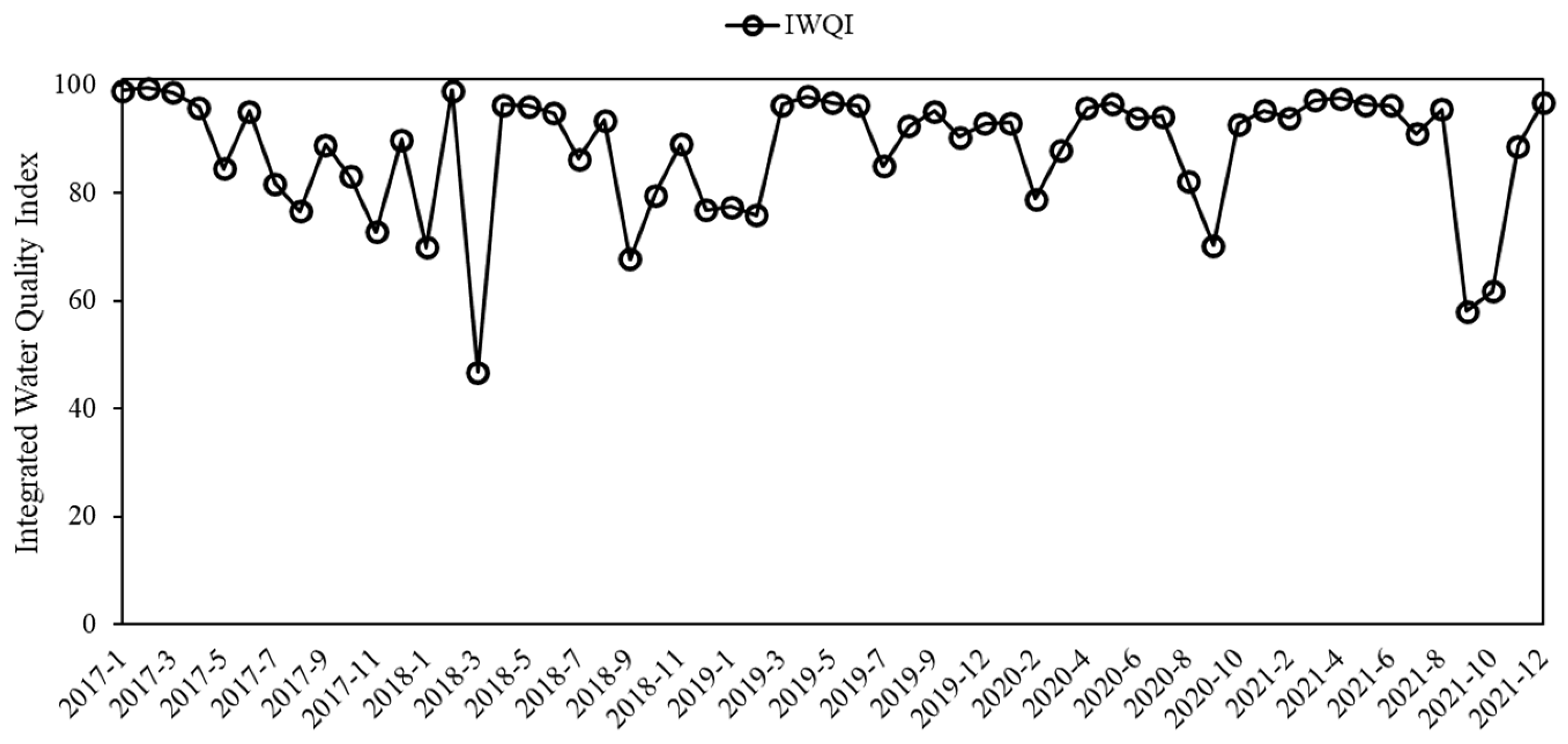
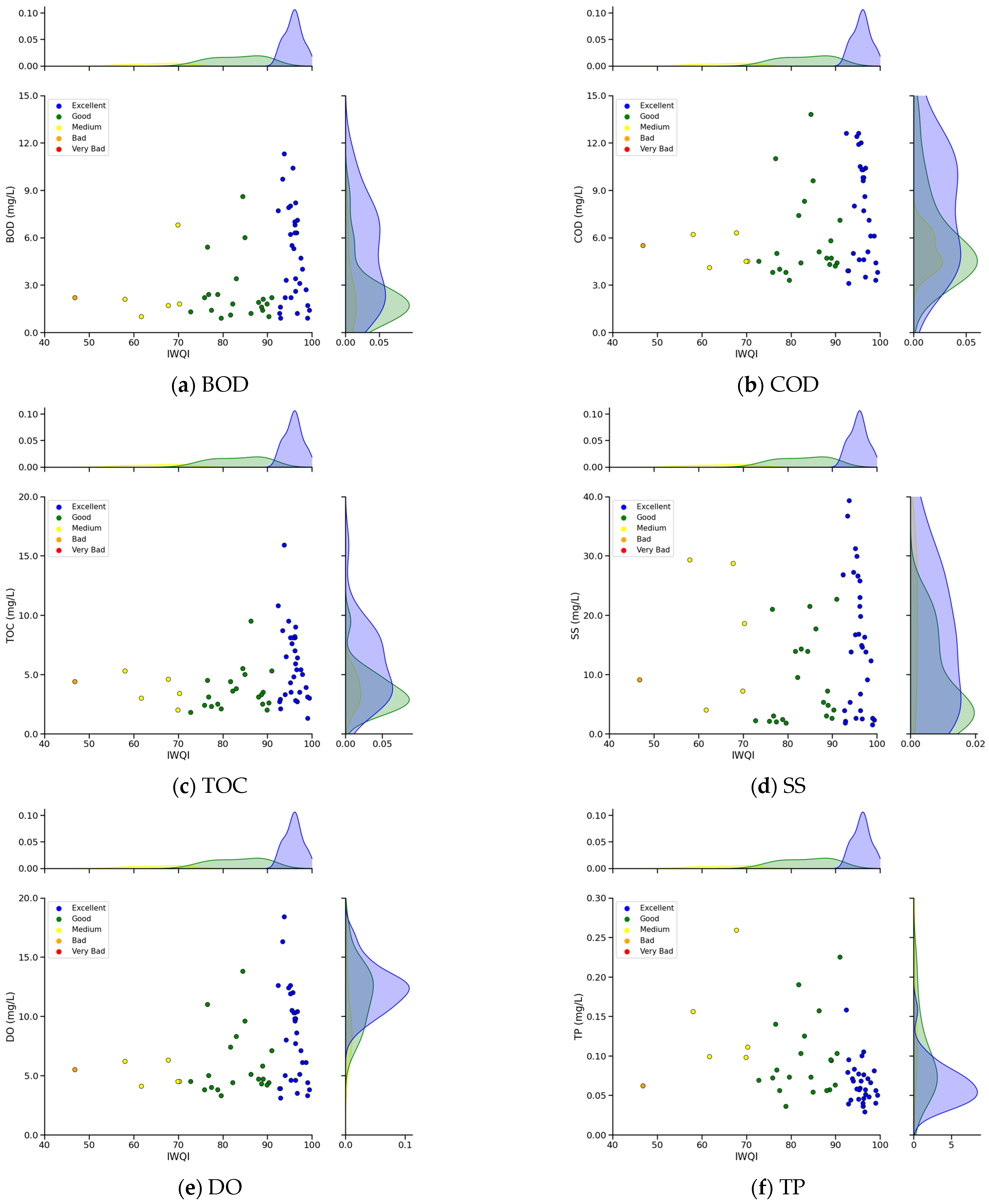
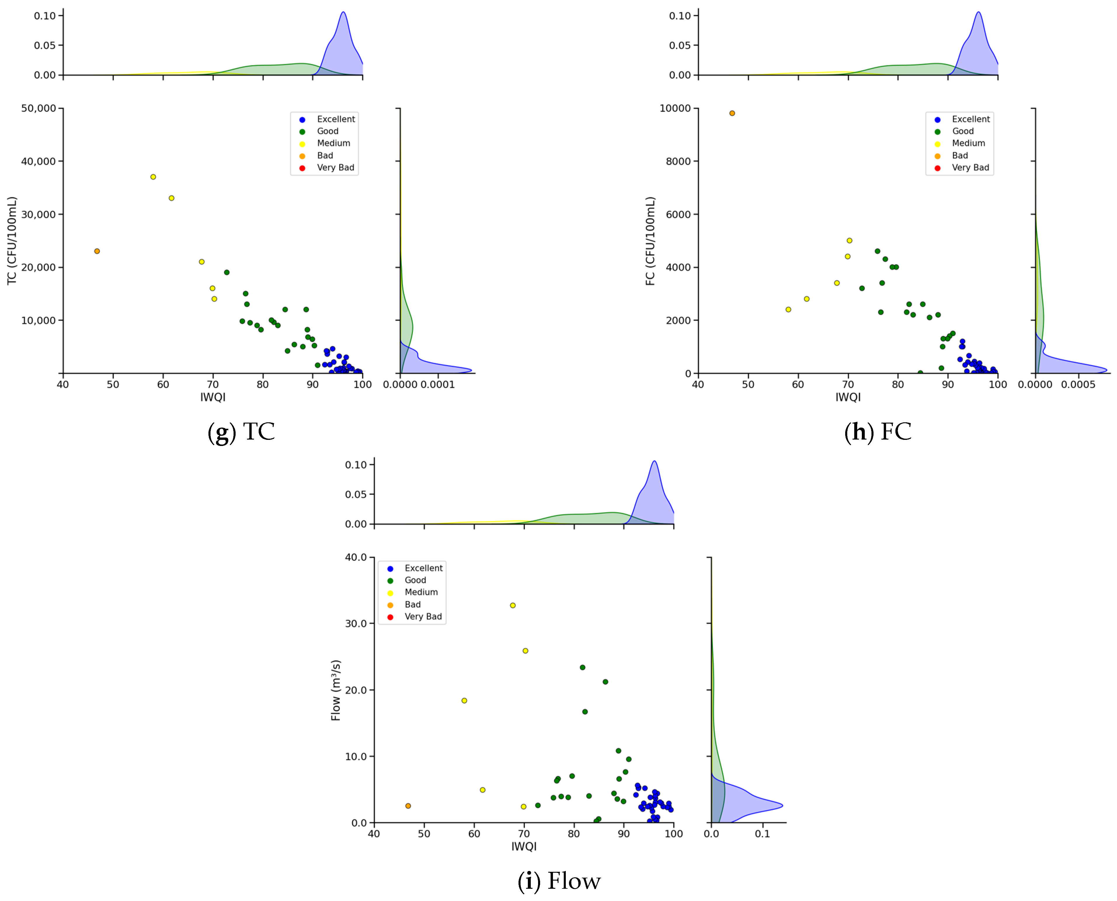
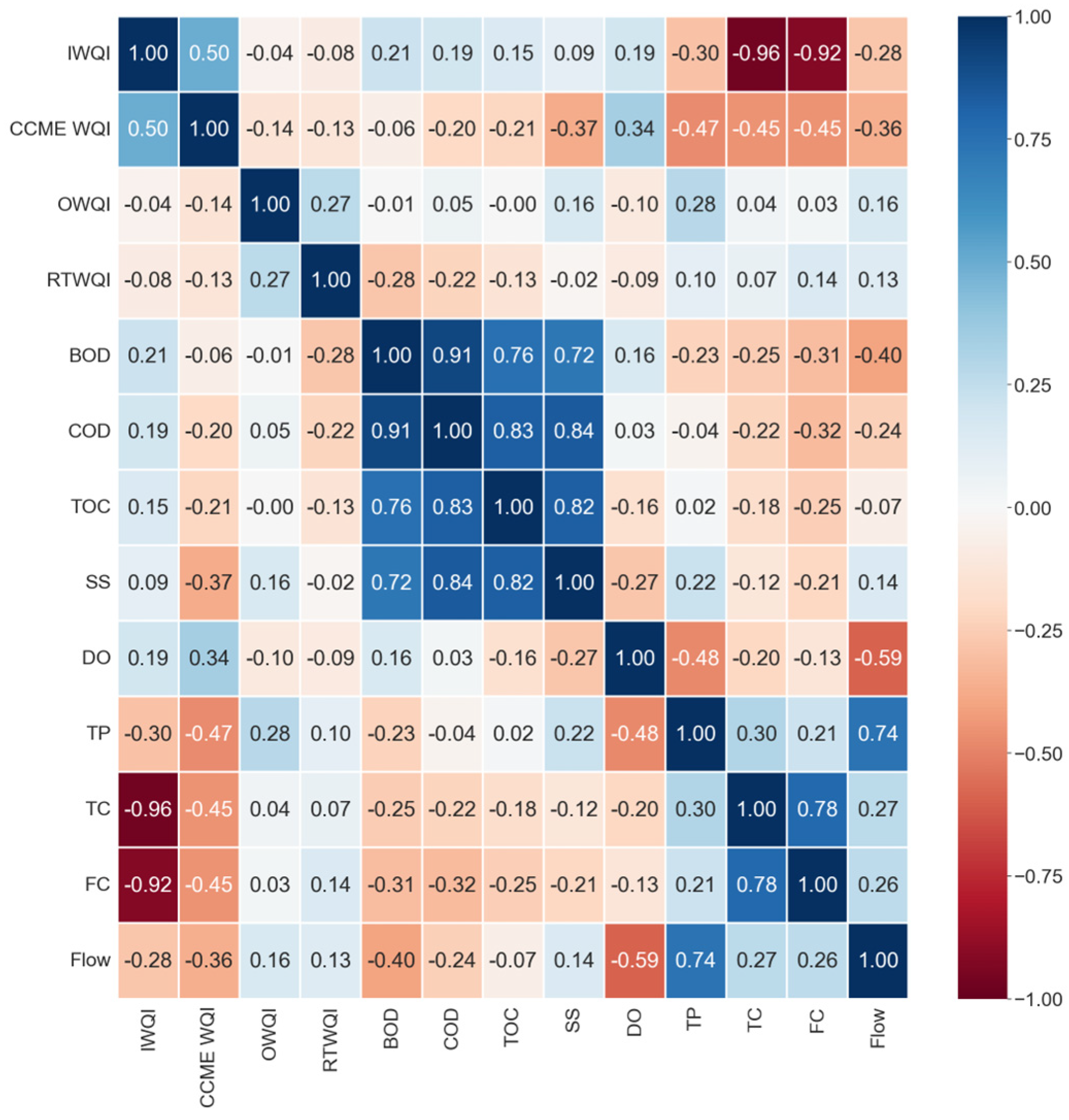
3.1. Comprehensive Evaluation of River Water Quality Using the IWQI

Factor Analysis (FA) was performed to apply weights to each parameter of the IWQI. Before conducting factor analysis, the Bartlett test and the Kaiser–Meyer–Olkin (KMO) test were conducted to evaluate the suitability of the data. The Bartlett test results showed a significance probability of less than 0.05, indicating a significant correlation. The KMO test resulted in a value of 0.727, demonstrating that the data were appropriate for performing factor analysis.
The extracted factor loadings for each factor were classified into parameters based on values above ±0.4 (Table 3). Factor 1 showed a significant correlation among the organic indicators BOD, COD, TOC, and SS. Factor 2 included DO, TP, and flow rate. The positive correlation between flow rate and TP indicated water quality changes due to flow rate fluctuations. In contrast, DO showed a negative correlation, suggesting seasonal characteristics where dissolved oxygen decreases in the summer. Factor 3 comprised TC and FC, which are microbial indicators and showed a low correlation with other water quality parameters.
To apply the factor analysis results as weights, the absolute value of the factor loadings approximated to ±1.0 was taken, and the relative weighting method was used to calculate the weight of each parameter (Table 4).
The IWQI was calculated using the weighted arithmetic average of the calculated weights. Considering flow fluctuations, the minimum value of the IWQI, calculated by combining the flow factor with the existing water quality index, was 49.4 points, and the maximum value was 3063.9 points. The score range was standardized from 0 to 100 using a rescaling method. The IWQI was evaluated by applying the five grades of the NSFWQI rating system: excellent (100–91), good (90–71), medium (70–51), bad (50–26), and very bad (25–0). The river water quality was overall good, with 33 instances rated as excellent, 19 as good, 4 as medium, and 1 as bad (Figure 4).
The IWQI was also evaluated based on the grading criteria used by other WQIs. The grading criteria for CCME WQI are as follows: 100–95 (excellent), 94–80 (good), 79–65 (fair), 64–45 (marginal), and 44–0 (poor). For the OWQI, the categories are 100–90 (excellent), 89–85 (good), 84–80 (fair), 79–60 (poor), and 59–10 (very poor). Meanwhile, the RTWQI uses the following ranges: 100–80 (excellent), 79–60 (good), 59–40 (fair), 39–20 (poor), and 19–0 (very poor). When compared to these indices, the IWQI grading scale evaluates water quality more leniently than the CCME WQI and OWQI but is relatively stricter than the RTWQI grading system (Table 5).
The relationship between the IWQI and the parameters was examined through scores, grades, and observations and was identified by referring to the results in Figure 2 (Figure 5). While BOD, COD, TOC, DO, and SS indicate high levels of water pollution, the IWQI is still evaluated as excellent. However, TP, TC, FC, and flow rate are observed at low values within the excellent grade. DO has minimal impact on the IWQI results, as all observed values meet the standard thresholds. SS is interpreted similarly to DO, showing low pollution levels. As the contamination levels of BOD, COD, and TOC increase, the IWQI score tends to rise. Conversely, the IWQI score increases for TP, TC, FC, and flow rate as their pollution levels decrease. This trend is evident in the results in Figure 2, where high pollution levels for TP, TC, and FC are observed during periods of high flow. Generally, the IWQI is designed to yield a higher score when parameters meet the standard values. TP, TC, FC, and flow rate show results that contrast with BOD, COD, and TOC, as pollution levels decrease with increased flow. According to the IWQI, the water quality of the Cheongmi River is significantly impacted by pollution related to TP, TC, FC, and flow rate, which suggests the need for targeted management strategies.
The CCME WQI was designed with the flexibility to select parameters freely, which allowed it to be aligned with the same parameters used in the IWQI. On the other hand, the OWQI and RTWQI were based on parameters shared with the IWQI from the ones proposed by their respective development agencies. The OWQI incorporated DO, BOD, TP, and TC from a broader set that included WT, pH, DO, BOD, TS, TP, TN, and TC. Meanwhile, the RTWQI utilized DO, TOC, and TP in its calculation.
To analyze the relationships among the indices, a Pearson correlation analysis was conducted between the IWQI, CCME WQI, OWQI, and RTWQI, along with the water quality parameters (Figure 6). The analysis revealed a strong negative correlation between the IWQI and TC (R2 = −0.96) and FC (R2 = −0.92), indicating that higher coliform levels lead to a significant decrease in IWQI scores. This highlights the crucial role of coliforms in degrading water quality as reflected by the IWQI. DO, BOD, COD, and TOC demonstrated a weak positive correlation with the IWQI (DO: R2 = 0.19, BOD: R2 = 0.21, COD: R2 = 0.19, TOC: R2 = 0.15). In contrast, flow showed a weak negative correlation (R2 = −0.28), and SS had a very weak positive correlation with the IWQI (R2 = 0.09), suggesting that these parameters exert a limited influence on IWQI scores. The CCME WQI exhibited similar correlations to the IWQI. It had a moderate positive correlation with the IWQI (R2 = 0.50) and a moderate negative correlation with TC and FC (R2 = −0.45 for both), mirroring the IWQI’s behavior. However, the OWQI and RTWQI displayed a very weak negative correlation with the IWQI (OWQI: R2 = −0.04, RTWQI: R2 = −0.08), with their correlations with individual parameters also being very weak (R2 ranging from 0.00 to −0.28). These weak correlations are likely due to differences in the selected parameters and the calculation methods used for each WQI. On the other hand, the CCME WQI, which uses the same parameters as the IWQI, shows improved correlations. Therefore, water quality assessment using the IWQI can be considered appropriate due to its stronger alignment with key water quality parameters compared to other indices.

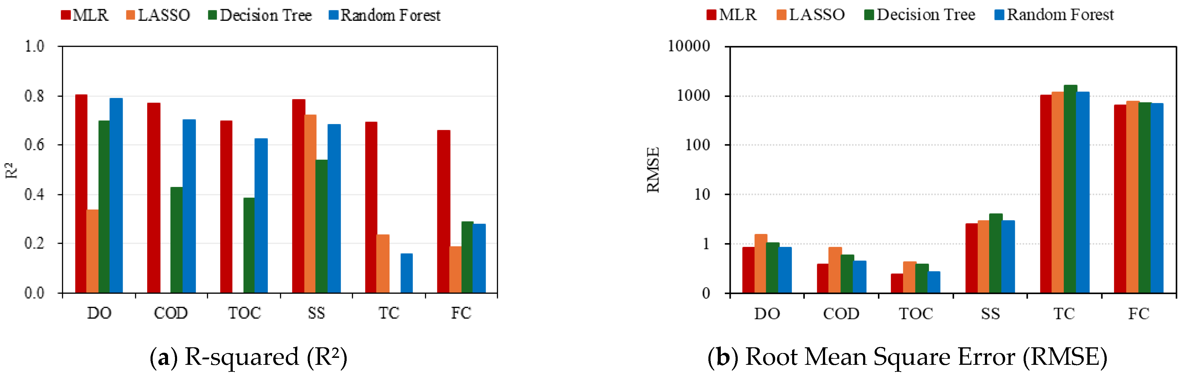
3.2. Evaluation of the Reproducibility of the Physics-Based and Data-Based Models

Calibration and verification were conducted to predict BOD and TP, as well as the flow rate and water quality of the Cheongmi River watershed. The verification period was set from 2017, when the integrated water quality index was calculated, to 2021, while the calibration period was set from 2012 to 2016 to match the verification period (Figure 7). The methods used to evaluate the reproducibility of the HSPF include % difference, NSE, R2, and PBIAS. In this study, among the reproducibility evaluation methods proposed by [70], the % difference, which is commonly used to evaluate flow rate, BOD, and TP, was applied to assess the reproducibility of simulated values. The % difference is categorized as follows: very good (less than 10), good (between 10 and 15), fair (between 15 and 25), and poor (greater than 25). Generally, the model’s reproducibility is considered appropriate when rated as good or higher.
The % difference for the flow rate during the calibration period was 7.0, and during the verification period, it was 9.5, indicating that the prediction reproducibility is appropriate. The % difference for BOD was 6.4 and 6.1 in the calibration and verification periods, respectively. For TP, the % difference was 13.4 during the calibration period and 13.8 during the verification period, Although the % difference for TP is relatively high compared to flow rate and BOD, it still satisfies the % difference standard.
Using the flow rate, BOD, and TP predicted by the HSPF from 2017 to 2021 as input variables, a regression model was applied to predict the DO, COD, TOC, SS, TC, and FC values required to calculate the integrated water quality index.
The data-based regression models employed multiple linear regression, LASSO regression, decision tree regression, and random forest regression. K-fold cross-validation was performed to select a model suitable for water quality prediction. Models trained with the same data tend to overfit through repeated patterns. K-fold cross-validation mitigates bias and variance by splitting the data for model verification into k subsets, iteratuvely performing training and testing [71]. In this study, K-fold cross-validation was performed with k = 5, and the reproducibility of the simulated water quality was quantitatively evaluated using R-squared (R2) and RMSE (Root Mean Square Error). R2 indicates the proportion of the variance in the dependent variable explained by the independent variables. In the R2 calculation formula, SSR represents the sum of squares due to regression, and SST represents the total sum of squares (Equation (7)). RMSE is a prediction performance indicator that measures the average error between predicted and actual values. Here, n refers to the number of data points, y i is the actual value, and y ^ i is the predicted value (Equation (8)).
R 2 = S S R S S T
R M S E = i = 1 n y i y ^ i 2 n
When comparing the four regression models, the multiple linear regression model and the random forest regression model showed excellent performance (Figure 8). The random forest regression model is insensitive to outliers and noise, efficiently processes predictors, and is effective at handling large data sets with fast calculation speeds [72]. However, random forest has the disadvantage of being a black-box model; although it offer high predictability, it is difficult to intuitively interpret the prediction results [73]. The multiple linear regression model, on the other hand, is characterized by its ease of interpretation, as it can clarify the relationship between independent variables and dependent variables [74]. Considering these advantages and disadvantages, we adopted the multiple linear regression model due to its relatively superior performance evaluation.

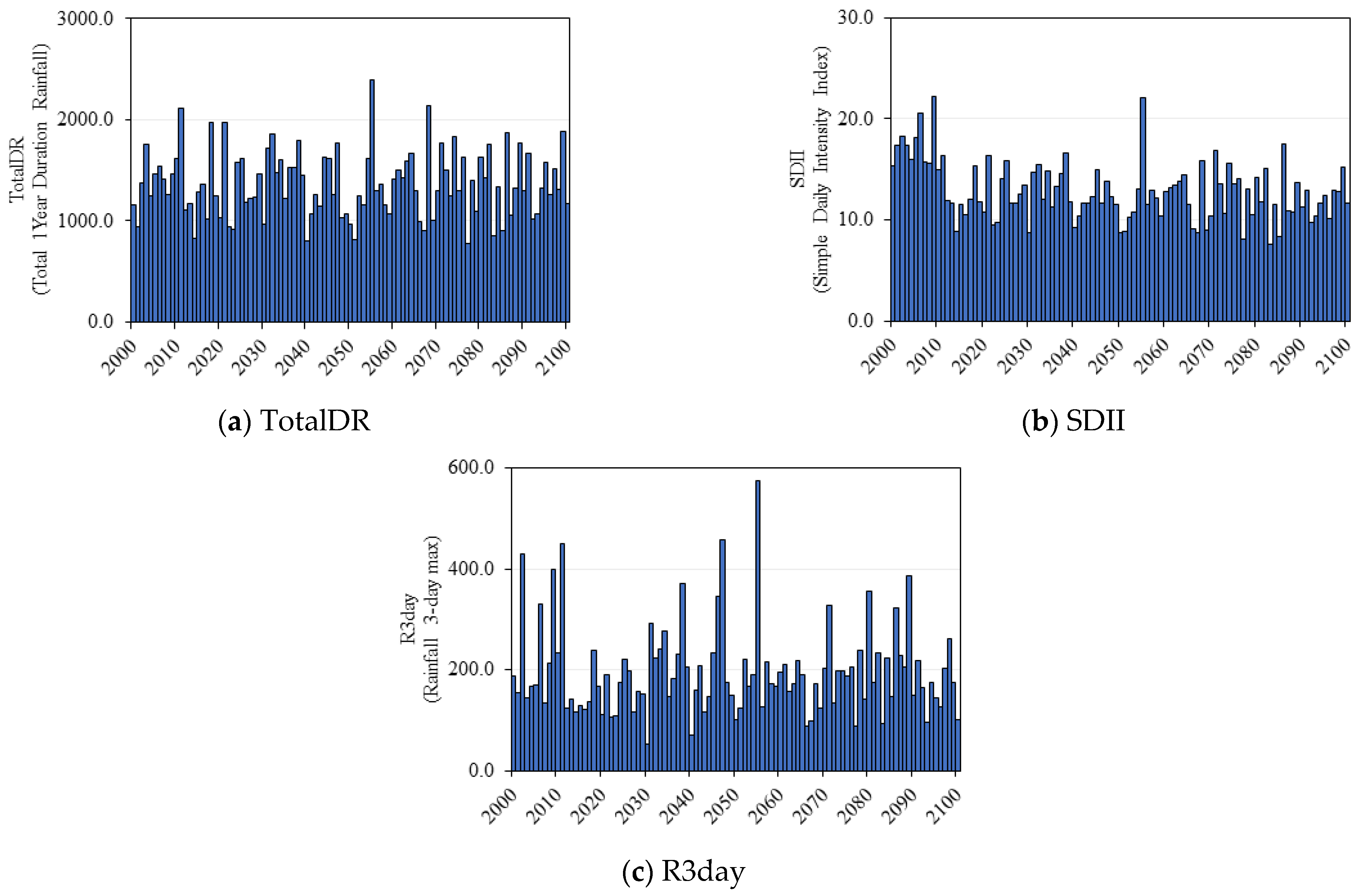
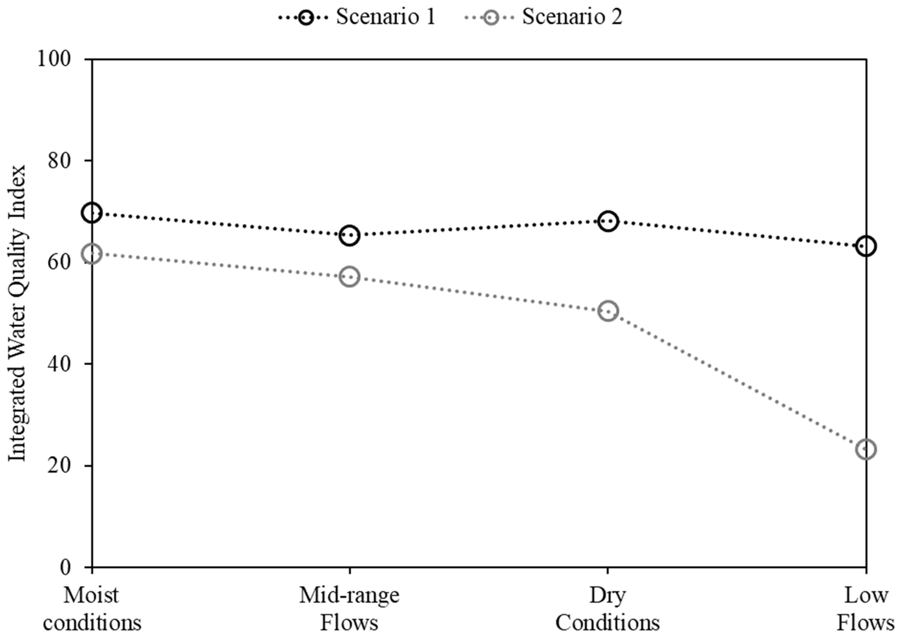
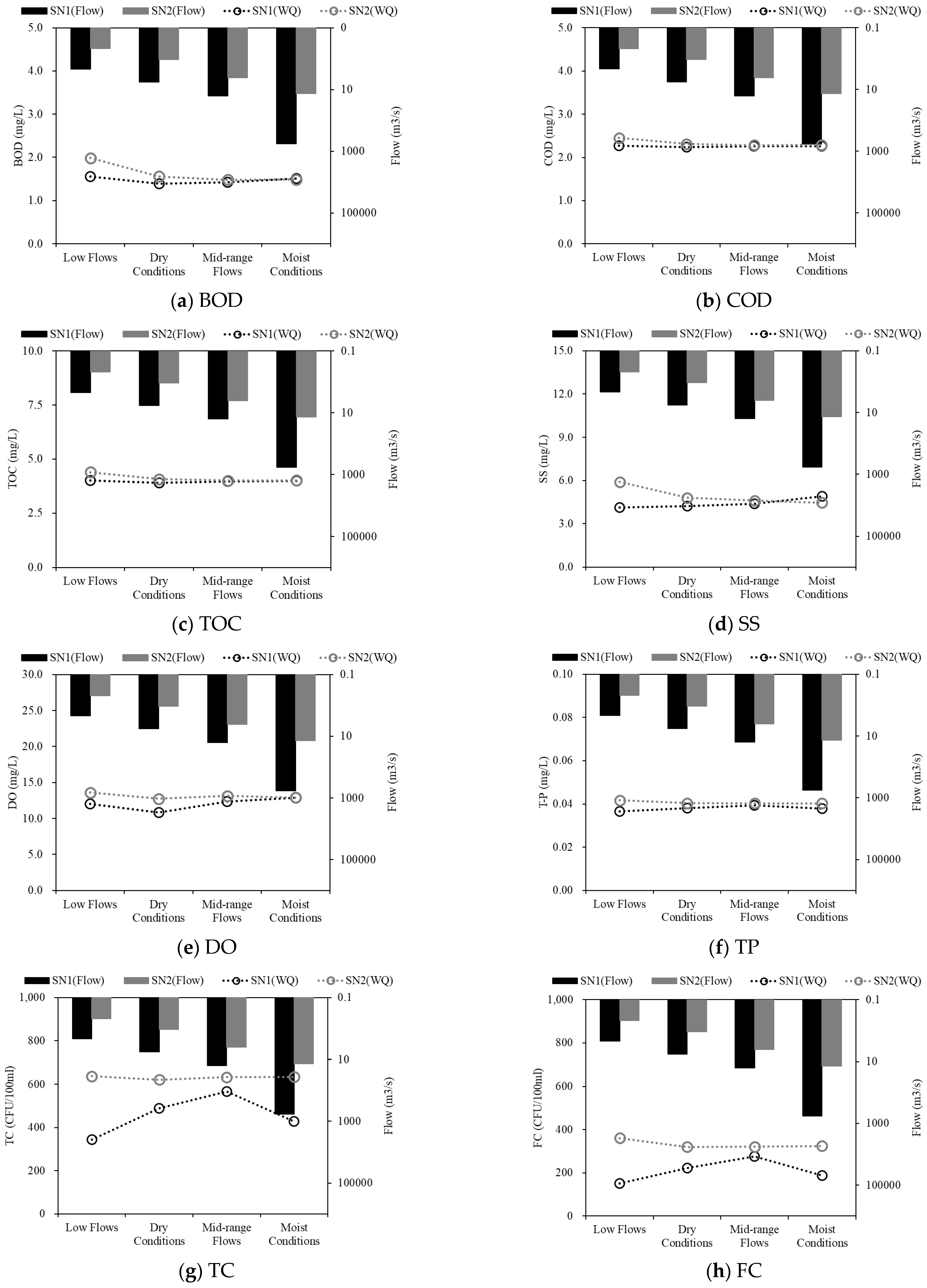
3.3. Evaluation of Climate Change Using the IWQI

To comprehensively evaluate river water quality due to climate change conditions, we reviewed the Intergovernmental Panel on Climate Change (IPCC) AR5 (RCPs) climate change scenarios and selected an appropriate scenario. These scenarios include RCP 2.6, RCP 4.5, RCP 6.0, and RCP 8.5, with the RCP 8.5 scenario assuming the highest emissions of greenhouse gases. For the target watershed, we selected the RCP 4.5 scenario, which reflects policies aimed at reducing greenhouse gas emissions [75]. Precipitation data provided in the RCP 4.5 scenario were compared using the precipitation index proposed by [76]. The rainfall indices used included TotalDR (Total 1-Year Duration Rainfall), SDII (Simple Daily Intensity Index), and R3day (3-Day Maximum Rainfall).
TotalDR is calculated as the total annual precipitation, SDII is calculated by dividing the total precipitation by the number of days with precipitation of 1 mm/day or more, and R3day is the maximum precipitation recorded over three consecutive days. In this study, we evaluated extreme precipitation events using these three types of precipitation indices (Figure 9). Using data from the Yangpyeong and Icheon observatories near the study watershed from 2000 to 2100, we calculated watershed precipitation and compared precipitation indices by year.
Scenario 1 (2055) was evaluated as having abundant precipitation with a TotalDR of 2387.6 mm/year, an SDII of 22.1 mm/day, and an R3day of 575.0 mm. Scenario 2 (2077) was evaluated as having insufficient precipitation with a TotalDR of 774.9 mm/year, an SDII of 8.1 mm/day, and an R3day of 89.1 mm.
The adopted scenario was applied as input to the HSPF and multiple linear regression models, which had completed reproducibility verification. To understand the river water quality management period, the entire period was divided into flow sections. Flow sections were distinguished by calculating the probability of exceeding the flow rate. The exceedance probability calculation is summarized in Equation (9). Daily flow data are sorted from maximum flow to minimum flow, and exceedance probabilities are calculated as percentages [77]. Flow sections are classified into moist conditions (10–40%), middle-range flows (40–60%), dry conditions (60–90%), and low flows (90–100%) [78].
F l o w   E x c e e d a n c e   P e r c e n t i l e % = R a n k   o f   d a t a / N u m b e r   o f   d a t a × 100
By applying climate change scenarios, the IWQI was calculated using BOD, COD, TOC, SS, DO, TP, TC, FC, and flow simulated with the HSPF and a multiple linear regression model. For each scenario, the daily IWQI was calculated based on one year of data. The calculated IWQI was then analyzed as the average value for each flow section (Figure 10). In scenario 1, where precipitation is abundant, the change in score is minimal as the flow section decreases, resulting in a consistent score range and being evaluated as medium. In scenario 2, where there is insufficient precipitation, the score tends to decrease as the flow section decreases, and the integrated water quality index rating dropped to very bad during the dry season, a time of water shortage. When comprehensively evaluating changes in flow rate and water quality due to climate change, it was determined that water quality deteriorates as the flow rate decreases.
We analyzed the impact on the integrated water quality index by comparing the water quality and flow rate across scenarios for each flow section (Figure 11). The flow rate for each scenario shows a rapid increase. In particular, in scenario 1, the flow rate varied significantly from 2.2 m3/s during the dry season to 576.5 m3/s during the rainy season. COD, TOC, DO, and TP tended to be insensitive to change in flow rate changes, while BOD, SS, TC, and FC were sensitive to water quality changes due to flow rate variations. BOD and SS tended to worsen in water quality as the flow rate decreased. For TC and FC, water quality concentration increased with rising flow rate in scenario 1, but water quality tended to improve during moist conditions and mid-range flows periods.
We also analyzed concentration differences between the scenarios for each water quality parameter. BOD and SS exhibited concentration changes of more than 11.0% from the low flows period, and TP showed a 12.4% change in water quality during the dry conditions period, indicating a deterioration in water quality in scenario 2. TC and FC exhibited relatively small changes of 10.0 to 14.0% during the normal season, but in other sections, they showed changes of 20.0 to 60.0%, indicating a serious deterioration in water quality in scenario 2.
When comparing water quality across scenarios based on flow rate section, water quality management is necessary starting from the dry conditions period. In particular, microbial indicators TC and FC were found to require intensive management. Therefore, it is essential to develop a feasible water quality management plan for river management during times of water shortage caused by low rainfall.

4. Conclusions

The results of this study highlight the importance of integrating flow with water quality parameters to develop comprehensive water quality assessment tools, especially in the context of climate change. The developed IWQI effectively addresses the limitations of traditional WQIs, which often overlook the significant impact of hydrological variability on water quality. The IWQI was formulated by modifying the NSFWQI method to include flow rate as a critical factor. Parameters such as DO, BOD, COD, SS, TOC, TP, TC, and FC were selected, and weights were calculated using FA. Including recalculated weights and flow rates allows for a more accurate reflection of water quality changes under different hydrological conditions.
The HSPF model was used to simulate flow and contaminant transport within the watershed. This model provided a robust framework for predicting water quality parameters under various climate scenarios. In this study, the RCP 4.5 scenario, which reflects a moderate greenhouse gas reduction policy, was applied to evaluate the impact of climate change on water quality. Using precipitation indices such as TotalDR, SDII, and R3day, the study assessed extreme precipitation events and their impact on water quality. Results indicate that traditional WQIs are inconsistent due to methodological differences and often fail to capture the impact of flow rate on water quality. In high-rainfall scenarios, water quality remained stable, but in low-rainfall scenarios, water quality deteriorated significantly during low-flow periods.
The IWQI was evaluated using various metrics, including the % difference. Both the multiple linear regression model and the random forest regression model demonstrated excellent performance in predicting water quality variables, with the former being adopted for its interpretability. The findings underscore the importance of targeted management strategies to address microbial and organic pollution, especially during periods of low rainfall. The IWQI provides a comprehensive tool for assessing and managing water quality and highlights the need for adaptation strategies to respond to hydrological changes due to climate change. The IWQI is a powerful tool for comprehensively assessing water quality, particularly when nonlinear modeling is employed to account for the complex and interrelated dynamics of the parameters involved. While it effectively captures the impacts of contaminants, oxygenation, and microbial pollution, its weaker correlation with parameters such as flow rate and SS suggests that systems dominated by physical processes could benefit from further refinement. This study presented a methodology to evaluate comprehensive river water quality by incorporating flow rate into the IWQI. However, the analysis was limited to the Cheongmi River, which may pose challenges in generalizing the findings to other watersheds. To verify the broader applicability of the IWQI, future research should expand the spatial scope by applying this methodology to various river watersheds with differing hydrological and environmental characteristics. This will allow for a more robust validation of the IWQI’s adaptability and reliability across diverse contexts, thereby ensuring its practical utility in water quality management beyond the current study area.
Future studies should explore the application of the IWQI in different watersheds and under various climate conditions to verify its robustness and adaptability. Integrating machine learning techniques and incorporating more complex climate variables can improve the prediction accuracy of the IWQI. Collaborating with policymakers to integrate the IWQI into water resource management frameworks can facilitate the development of effective strategies to maintain water quality under changing environmental conditions.
In conclusion, the IWQI developed in this study integrates flow rate to provide a more holistic and accurate assessment of river water quality, addressing significant gaps in traditional WQIs. This integrated approach is essential for effective water resource management, especially in the context of increasing climate variability and its impacts on hydrology and water dynamics.

Author Contributions

Conceptualization, S.L. and B.G.J.; methodology, S.L.; software, J.M.L.; validation, J.M.L.; formal analysis, S.L. and B.G.J.; investigation, S.L. and J.L.; resources, Y.D.K.; data curation, S.L. and B.G.J.; writing—original draft preparation, S.L.; writing—review and editing, Y.D.K.; visualization, S.L. and J.L.; supervision, Y.D.K.; project administration, Y.D.K.; funding acquisition, Y.D.K. All authors have read and agreed to the published version of the manuscript.

Funding

Research and Development on the Technology for Securing the Water Resources Stability in Response to Future Change of the Ministry of Environment, grant number RS-2024-00332114.

Data Availability Statement

The original contributions presented in this study are included in the article. Further inquiries can be directed to the corresponding author(s).

Acknowledgments

The authors gratefully acknowledge the graduate students and researcher of Myongji University and the researcher of the National Institute of Environmental Research.

Conflicts of Interest

The authors declare no conflict of interest.

References

  1. Mukate, S.; Wagh, V.; Panaskar, D.; Jacobs, J.A.; Sawant, A. Development of new integrated water quality index (IWQI) model to evaluate the drinking suitability of water. Ecol. Indic. 2019, 101, 348–354. [Google Scholar] [CrossRef]
  2. Lee, J.H.; Ha, H.J.; Lee, M.H.; Lee, M.Y.; Kim, T.H.; Cha, Y.K.; Koo, J.Y. Assessment of water quality of major tributaries in Seoul using water quality index and cluster analysis. J. Korean Soc. Environ. Eng. 2020, 42, 452–462. [Google Scholar] [CrossRef]
  3. Uddin, M.G.; Nash, S.; Olbert, A.I. A review of water quality index models and their use for assessing surface water quality. Ecol. Indic. 2021, 122, 107218. [Google Scholar] [CrossRef]
  4. Apogba, J.N.; Anornu, G.K.; Koon, A.B.; Dekongmen, B.W.; Sunkari, E.D.; Fynn, O.F.; Kpiebaya, P. Application of machine learning techniques to predict groundwater quality in the Nabogo Basin. North. Ghana Heliyon 2024, 10, e28527. [Google Scholar] [CrossRef] [PubMed]
  5. Lap, B.Q.; Phan, T.; Du Nguyen, H.; Hang, P.T.; Phi, N.Q.; Hoang, V.T.; Linh, P.G.; Hang, B.T.T. Predicting Water Quality Index (WQI) by feature selection and machine learning: A case study of An Kim Hai irrigation system. Ecol. Inform. 2023, 74, 101991. [Google Scholar] [CrossRef]
  6. Azha, S.F.; Sidek, L.M.; Ahmad, Z.; Zhang, J.; Basri, H.; Zawawi, M.H.; Noh, N.M.; Ahmed, A.N. Enhancing river health monitoring: Developing a reliable predictive model and mitigation plan. Ecol. Indic. 2023, 156, 111190. [Google Scholar] [CrossRef]
  7. Park, K.D.; Kang, D.H.; So, Y.H.; Kim, I.K. Temporal-spatial variations of water quality level and water quality index on the living environmental standards in the west Nakdong River. J. Environ. Sci. Int. 2019, 28, 1071–1083. [Google Scholar] [CrossRef]
  8. Nayak, J.G.; Patil, L.G.; Patki, V.K. Development of water quality index for Godavari River (India) based on fuzzy inference system. Groundw. Sustain. Dev. 2020, 10, 100350. [Google Scholar] [CrossRef]
  9. Tyagi, S.; Sharma, B.; Singh, P.; Dobhal, R. Water quality assessment in terms of water quality index. Am. J. Water Resour. 2013, 1, 34–38. [Google Scholar] [CrossRef]
  10. Park, J.; Kal, B.; Kim, S. Long-term trend analysis of major tributaries of Nakdong River using water quality index. J. Wetl. Res. 2018, 20, 201–209. [Google Scholar]
  11. Gupta, S.; Gupta, S.K. A critical review on water quality index tool: Genesis, evolution and future directions. Ecol. Inform. 2021, 63, 101299. [Google Scholar] [CrossRef]
  12. Darvishi, G.; Kootenaei, F.G.; Ramezani, M.; Lotfi, E.; Asgharnia, H. Comparative investigation of river water quality by OWQI, NSFWQI and Wilcox indexes (Case study: The Talar River—Iran). Arch. Environ. Prot. 2016, 42, 41–48. [Google Scholar] [CrossRef]
  13. Kalagbor, I.A.; Johnny, V.I.; Ogbolokot, I.E. Application of national sanitation foundation and weighted arithmetic water quality indices for the assessment of Kaani and Kpean Rivers in Nigeria. Am. J. Water Resour. 2019, 7, 11–15. [Google Scholar]
  14. Zotou, I.; Tsihrintzis, V.A.; Gikas, G.D. Performance of seven water quality indices (WQIs) in a Mediterranean river. Environ. Monit. Assess. 2019, 191, 505. [Google Scholar] [CrossRef]
  15. Kim, Y.T.; Park, M.; Kwon, H.H. Spatio-temporal summer rainfall pattern in 2020 from a rainfall frequency perspective. J. Korean Soc. Disaster Secur. 2020, 13, 93–104. [Google Scholar]
  16. Park, J.E.; Kim, H.N.; Ryoo, K.S.; Lee, E.R. Evaluation of flexible criteria for river flow management with consideration of spatio-temporal flow variation. J. Korea Water Resour. Assoc. 2016, 49, 673–683. [Google Scholar] [CrossRef]
  17. Jang, S.H.; Lee, J.K.; Jo, J.W. Evaluation of instream flow in the Imjingang River according to the operation of Hwanggang Dam in North Korea. Crisis Emerg. Manag. Theory Prax. 2020, 16, 105–118. [Google Scholar] [CrossRef]
  18. Cho, Y.H.; Park, S.Y.; Na, J.M.; Kim, T.W.; Lee, J.H. Hydrological and ecological alteration of river dynamics due to multipurpose dams. J. Wetl. Res. 2019, 21, 16–27. [Google Scholar]
  19. Jun, H.; Kim, S. Analysis of future hydrological cycle considering the impact of climate change and hydraulic structures in Geum River Basin. J. Korean Soc. Hazard Mitig. 2014, 14, 299–309. [Google Scholar] [CrossRef]
  20. Chang, I.S.; Jung, J.K.; Park, K.B. Analysis of correlation relationship for flow and water quality at up and down streams. J. Environ. Sci. Int. 2010, 19, 771–778. [Google Scholar]
  21. Cho, H.K. A study on the related characteristics of discharge-water quality in Nakdong river. J. Environ. Sci. Int. 2011, 20, 373–384. [Google Scholar] [CrossRef]
  22. Cho, Y.C.; Park, M.; Shin, K.; Choi, H.M.; Kim, S.; Yu, S. A study on grade classification for improvement of water quality and water quality characteristics in the Han River watershed tributaries. J. Environ. Impact Assess. 2019, 28, 215–230. [Google Scholar]
  23. Woo, S.Y.; Kim, S.J.; Hwang, S.J.; Jung, C.G. Assessment of changes on water quality and aquatic ecosystem health in Han River basin by additional dam release of stream maintenance flow. J. Korea Water Resour. Assoc. 2019, 52, 777–789. [Google Scholar]
  24. Byun, J.; Son, M. Effects of climate change and reduction method on water quality in Cheongmicheon watershed. J. Korea Water Resour. Assoc. 2018, 51, 585–597. [Google Scholar]
  25. Kong, D.; Min, J.K.; Byeon, M.; Park, H.K.; Cheon, S.U. Temporal and spatial characteristics of water quality in a river-reservoir (Paldang). J. Korean Soc. Water Environ. 2018, 34, 470–486. [Google Scholar]
  26. Lee, S.; Lee, S. The analysis of water factors for management of lake eutrophication in Paldang lake. J. Korean Ecol. Eng. Soc. 2022, 9, 61–72. [Google Scholar]
  27. Kim, S.; Hwang, S.; Kim, S.; Lee, H.; Kwak, J.; Kim, J.; Kang, M. Evaluation of estuary reservoir management based on robust decision making considering water use-flood control-water quality under Climate Change. J. Korea Water Resour. Assoc. 2023, 56, 419–429. [Google Scholar]
  28. Yu, S.; Im, J.; Lee, B. Effect of air temperature changes on water temperature and hysteresis phenomenon in lake Paldang. J. Environ. Impact Assess. 2020, 29, 323–337. [Google Scholar]
  29. Kong, D. Evaluating effect of density flow from upstream on vertical distribution of water quality at the Paldang Reservoir. J. Korean Soc. Water Environ. 2019, 35, 557–566. [Google Scholar]
  30. Kim, J.K.; Lee, S.H.; Bang, H.H.; Hwang, S.O. Characteristics of algae occurrence in Lake Paldang. J. Korean Soc. Environ. Eng. 2009, 31, 325–331. [Google Scholar]
  31. Ryu, I.G.; Lee, B.M.; Cho, Y.C.; Choi, H.J.; Shin, D.S.; Kim, S.H.; Yu, S.J. Analyzing Flow Variation and Stratification of Paldang Reservoir Using High-frequency Water Temperature Data. J. Korean Soc. Water Environ. 2020, 36, 392–404. [Google Scholar]
  32. Hwang, S.J.; Kim, K.; Park, C.; Seo, W.; Choi, B.G.; Eum, H.S.; Park, M.H.; Noh, H.R.; Sim, Y.B.; Shin, J.K. Hydro-meteorological effects on water quality variability in Paldang reservoir, confluent area of the South-Han River-North-Han River-Gyeongan Stream, Korea. Korean J. Ecol. Environ. 2016, 49, 354–374. [Google Scholar] [CrossRef]
  33. Lee, S.; Shin, J.Y.; Lee, G.; Sung, Y.; Kim, K.; Lim, K.J.; Kim, J. Analysis of Water Pollutant Load Characteristics and Its Contributions During Dry Season: Focusing on Major Streams Inflow into South-Han River of Chungju-dam Downstream. J. Korean Soc. Environ. Eng. 2018, 40, 247–257. [Google Scholar] [CrossRef]
  34. Cho, Y.C.; Choi, H.M.; Ryu, I.G.; Kim, S.H.; Shin, D.; Yu, S. Assessment of water quality in the lower reaches Namhan River by using statistical analysis and water quality index (WQI). J. Korean Soc. Water Environ. 2021, 37, 114–127. [Google Scholar]
  35. Kim, Y.S.; Kim, S.H.; Lee, C.H. Tracing Water Pollution Source using FDC and Exceedance Rate in Cheongmicheon Watershed. J. Wetl. Res. 2018, 20, 136–144. [Google Scholar]
  36. Choi, M.; Jung, W.; Hwang, H.; Kim, Y. Water Quality Improvement Plans of Daeho Reservoir based on the Analysis of Watershed Characteristics and Water Quality Modelling. J. Korean Soc. Environ. Eng. 2018, 40, 267–276. [Google Scholar] [CrossRef]
  37. Lee, S.; Jo, B.; Kim, Y.D. Assessment of water quality index suitability of domestic watersheds. J. Korea Water Resour. Assoc. 2022, 55, 371–381. [Google Scholar]
  38. Yeon, I.S.; Ahn, S.J. A Development of Real Time Artificial Intelligence Warning System Linked Discharge and Water Quality (I) Application of Discharge-Water Quality Forecasting Model. J. Korea Water Resour. Assoc. 2005, 38, 565–574. [Google Scholar] [CrossRef]
  39. Banda, T.D.; Kumarasamy, M.V. Development of Water Quality Indices (WQIs): A Review. Pol. J. Environ. Stud. 2020, 29, 2011–2021. [Google Scholar] [CrossRef]
  40. Yan, F.; Qiao, D.; Qian, B.; Ma, L.; Xing, X.; Zhang, Y.; Wang, X. Improvement of CCME WQI using grey relational method. J. Hydrol. 2016, 543, 316–323. [Google Scholar] [CrossRef]
  41. Ramakrishnaiah, C.R.; Sadashivaiah, C.; Ranganna, G. Assessment of water quality index for the groundwater in Tumkur Taluk, Karnataka State, India. J. Chem. 2009, 6, 523–530. [Google Scholar] [CrossRef]
  42. Kim, M.C.; Kim, H.J.; Park, K.H.; Youn, H.K.; Lee, S.H. Analysis of fire risk assessment indicators of publicly-used establishments using Delphi/AHP. Fire Sci. Eng. 2019, 33, 87–94. [Google Scholar] [CrossRef]
  43. Yoo, D.G.; Jun, H.D.; Jung, D.H.; Kim, J.H. Suggestion of Weighted Utopian Approach for Combining Weighting Methods and Utopian Approach. J. Korean Soc. Hazard Mitig. 2010, 10, 119–125. [Google Scholar]
  44. Hou, W.; Sun, S.; Wang, M.; Li, X.; Zhang, N.; Xin, X.; Sun, L.; Li, W.; Jia, R. Assessing water quality of five typical reservoirs in lower reaches of Yellow River, China: Using a water quality index method. Ecol. Indic. 2016, 61, 309–316. [Google Scholar] [CrossRef]
  45. Jahin, H.S.; Abuzaid, A.S.; Abdellatif, A.D. Using multivariate analysis to develop irrigation water quality index for surface water in Kafr El-Sheikh Governorate, Egypt. Environ. Technol. Innov. 2020, 17, 100532. [Google Scholar] [CrossRef]
  46. Sutadian, A.D.; Muttil, N.; Yilmaz, A.G.; Perera, B.J.C. Development of river water quality indices—A review. Environ. Monit. Assess. 2016, 188, 58. [Google Scholar] [CrossRef]
  47. Park, J.; Moon, M.; Lee, H.; Kim, K. A study on characteristics of water quality using multivariate analysis in Sumjin River basin. J. Korean Soc. Water Environ. 2014, 30, 119–127. [Google Scholar] [CrossRef]
  48. Park, J.; Kal, B.; Kim, S. Application of multivariate statistical techniques to analyze the pollution characteristics of major tributaries of the Nakdong River. J. Wetl. Res. 2019, 21, 215–223. [Google Scholar]
  49. Kwon, P.S.; Park, M.J.; Lee, Y.J.; Cho, Y.C.; Noh, C.W.; Jung, W.S.; Kim, J.H.; Yu, S.J. Evaluation of water quality characteristics at Kyeongan stream using the flow-loading equation and factor analysis. Ecol. Resilient Infrastruct. 2017, 4, 226–236. [Google Scholar]
  50. Kim, S.M.; Park, S.W. Calibration and Validation of HSPF Mode1 to Estimate the Pollutant Loads from Rural Small Watershed. J. Korea Water Resour. Assoc. 2004, 37, 643–651. [Google Scholar] [CrossRef]
  51. Cho, H.K.; Kim, S.M. Estimation of the Hapcheon dam inflow using HSPF model. J. Korean Soc. Agric. Eng. 2019, 61, 69–77. [Google Scholar]
  52. Lee, S.; Kim, J.M.; Shin, H.S.; Kwon, S. Evaluation of riparian buffer for the reduction efficiency of non-point sources using HSPF Model. J. Korean Soc. Hazard Mitig. 2019, 19, 341–349. [Google Scholar] [CrossRef]
  53. Kwon, S.H.; Chung, G. Estimation of snow damages using multiple regression model-The case of gangwon province. KSCE J. Civ. Environ. Eng. Res. 2017, 37, 61–72. [Google Scholar]
  54. Peng, C.Y.J.; Lee, K.L.; Ingersoll, G.M. An introduction to logistic regression analysis and reporting. J. Educ. Res. 2002, 96, 3–14. [Google Scholar] [CrossRef]
  55. Oh, Y.H. High-school baseball pitcher’s ERA (Earned Run Average) prediction using multi-variable linear regression analysis method. J. Knowl. Inf. Technol. Syst. 2020, 14, 497–506. [Google Scholar]
  56. Kwon, S.H.; Lee, J.; Chung, G. Snow damages estimation using artificial neural network and multiple regression analysis. J. Korean Soc. Hazard Mitig. 2017, 17, 315–325. [Google Scholar] [CrossRef]
  57. Ryu, N.; Kim, H.; Kang, P. Evaluating variable selection techniques for multivariate linear regression. J. Korean Inst. Ind. Eng. 2016, 42, 314–326. [Google Scholar]
  58. Choi, S.Y.; Han, K.Y.; Kim, B.H. Comparison of different multiple linear regression models for real-time flood stage forecasting. KSCE J. Civ. Environ. Eng. Res. 2012, 32, 9–20. [Google Scholar]
  59. Zhao, Y.; Huo, X. Accelerate the warm-up stage in the Lasso computation via a homotopic approach. Comput. Stat. Data Anal. 2023, 184, 107747. [Google Scholar] [CrossRef]
  60. Yan, Z.; Yao, Y. Variable selection method for fault isolation using least absolute shrinkage and selection operator (LASSO). Chemom. Intell. Lab. Syst. 2015, 146, 136–146. [Google Scholar] [CrossRef]
  61. Mozafari, Z.; Chamjangali, M.A.; Arashi, M. Combination of least absolute shrinkage and selection operator with Bayesian Regularization artificial neural network (LASSO-BR-ANN) for QSAR studies using functional group and molecular docking mixed descriptors. Chemom. Intell. Lab. Syst. 2020, 200, 103998. [Google Scholar] [CrossRef]
  62. Liu, S.; Huang, Q.; Li, M.; Wei, Y. A new LASSO-BiLSTM-based ensemble learning approach for exchange rate forecasting. Eng. Appl. Artif. Intell. 2024, 127, 107305. [Google Scholar] [CrossRef]
  63. Zagow, M.; Elbany, M.; Darwish, A.M. Identifying urban, transportation, and socioeconomic characteristics across US zip codes affecting CO2 emissions: A decision tree analysis. Energy Built Environ. 2024; in press. [Google Scholar] [CrossRef]
  64. Díaz-Ramírez, J.; Estrada-García, J.A.; Figueroa-Sayago, J. Predicting transport mode choice preferences in a university district with decision tree-based models. City Environ. Interact. 2023, 20, 100118. [Google Scholar] [CrossRef]
  65. Dang, B.L.; Nguyen-Xuan, H.; Wahab, M.A. An effective approach for VARANS-VOF modelling interactions of wave and perforated breakwater using gradient boosting decision tree algorithm. Ocean Eng. 2023, 268, 113398. [Google Scholar] [CrossRef]
  66. Hou, T.; Sun, W.; Chen, C.; Yang, G.; Meng, X.; Peng, J. Marine floating raft aquaculture extraction of hyperspectral remote sensing images based decision tree algorithm. Int. J. Appl. Earth Obs. Geoinf. 2022, 111, 102846. [Google Scholar] [CrossRef]
  67. Zhang, H.; Wu, P.; Yin, A.; Yang, X.; Zhang, M.; Gao, C. Prediction of soil organic carbon in an intensively managed reclamation zone of eastern China: A comparison of multiple linear regressions and the random forest model. Sci. Total Environ. 2017, 592, 704–713. [Google Scholar] [CrossRef]
  68. Poddar, A.; Rangwani, N.; Palekar, S.; Kalambe, J. Glucose Monitoring System Using Machine Learning. Mater. Today Proc. 2023, 73, 100–107. [Google Scholar] [CrossRef]
  69. Rouabah, A.; Meiss, H.; Villerd, J.; Lasserre-Joulin, F.; Tosser, V.; Chabert, A.; Therond, O. Predicting the abundances of aphids and their natural enemies in cereal crops: Machine-learning versus linear models. Biol. Control 2022, 169, 104866. [Google Scholar] [CrossRef]
  70. Moriasi, D.N.; Gitau, M.W.; Pai, N.; Daggupati, P. Hydrologic and water quality models: Performance measures and evaluation criteria. Trans. ASABE 2015, 58, 1763–1785. [Google Scholar]
  71. Toft, H.B.; Müller, K.; Hendrikx, J.; Jaedicke, C.; Bühler, Y. Can big data and random forests improve avalanche runout estimation compared to simple linear regression? Cold Reg. Sci. Technol. 2023, 211, 103844. [Google Scholar] [CrossRef]
  72. Gounaridis, D.; Koukoulas, S. Urban land cover thematic disaggregation, employing datasets from multiple sources and RandomForests modeling. Int. J. Appl. Earth Obs. Geoinf. 2016, 51, 1–10. [Google Scholar] [CrossRef]
  73. Yuchi, W.; Gombojav, E.; Boldbaatar, B.; Galsuren, J.; Enkhmaa, S.; Beejin, B.; Naidan, G.; Ochir, C.; Legtseg, B.; Byambaa, T.; et al. Evaluation of random forest regression and multiple linear regression for predicting indoor fine particulate matter concentrations in a highly polluted city. Environ. Pollut. 2019, 245, 746–753. [Google Scholar] [CrossRef] [PubMed]
  74. Rokde, J.R.; Thosar, A.G. Linear regression approach for performance evaluation of ES with load impedance variations of non-critical and critical load. e-Prime-Advances in Electrical Engineering. Electron. Energy 2023, 6, 100312. [Google Scholar]
  75. Park, J.; Kang, M.S.; Song, I.; Hwang, S.H.; Song, J.H. Development of IDF curves based on RCP4. 5 scenario for 30-reservoirs in South Korea. J. Korean Soc. Hazard Mitig. 2013, 13, 145–160. [Google Scholar] [CrossRef]
  76. Lee, S.; Jo, B.; Kim, Y.D.; Lee, J.H. Analysis of effects of drought on water quality using HSPF and QUAL-MEV. J. Korea Water Resour. Assoc. 2023, 56, 393–402. [Google Scholar]
  77. Lee, S.; Kang, J.; Park, H.; Kang, J.; Kim, S.; Kim, J.P.; Kim, G. A study on the variation of water quality and the evaluation of target water quality using LDC in major tributaries of Nakdong river basin. J. Korean Soc. Water Environ. 2020, 36, 521–534. [Google Scholar]
  78. Lee, E.J.; Kim, T.G.; Keum, H.J. Application of FDC and LDC using HSPF model to support total water load management system. J. Korean Soc. Water Environ. 2018, 34, 33–45. [Google Scholar]
Figure 1. Location of measurement stations.
Hydrology 11 00178 g001
Figure 2. Analysis of water quality and flow rate distribution (a) BOD-flow rate relationship, (b) COD-flow rate relationship, (c) TOC-flow rate relationship, (d) SS-flow rate relationship, (e) DO-flow rate relationship, (f) TP-flow rate relationship, (g) TC-flow rate relationship, (h) FC-flow rate relationship.
Hydrology 11 00178 g002aHydrology 11 00178 g002b
Figure 3. Proposed Integrated Water Quality Index (IWQI) development framework.
Hydrology 11 00178 g003
Figure 4. IWQI scores for the Cheongmicheon watershed.
Hydrology 11 00178 g004
Figure 5. Comparison of IWQI trends with parameters (a) BOD-IWQI relationship, (b) COD-IWQI relationship, (c) TOC-IWQI relationship, (d) SS-IWQI relationship, (e) DO-IWQI relationship, (f) TP-IWQI relationship, (g) TC-IWQI relationship, (h) FC-IWQI relationship, (i) Flow rate-IWQI relationship.
Hydrology 11 00178 g005aHydrology 11 00178 g005b
Figure 6. Correlation Between IWQI, CCME WQI, OWQI, RTWQI and parameters.
Hydrology 11 00178 g006
Figure 7. Simulation results using HSPF: (a) Flow rate, (b) BOD, (c) TP.
Hydrology 11 00178 g007
Figure 8. Evaluation of regression models based on water quality parameter prediction performance (a) R2 of models by parameter, (b) RMSE of models by parameter.
Hydrology 11 00178 g008
Figure 9. Calculation of precipitation indices by climate and province (a) TotalDR calculated annually, (b) SDII calculated annually, (c) R3day calculated annually.
Hydrology 11 00178 g009
Figure 10. Assessment of climate change using IWQI.
Hydrology 11 00178 g010
Figure 11. Impact of water quality and flow by flow section under different scenarios (a) Change in BOD by scenarios, (b) Change in COD by scenarios, (c) Change in TOC by scenarios, (d) Change in SS by scenarios, (e) Change in DO by scenarios, (f) Change in TP by scenarios, (g) Change in TC by scenarios, (h) Change in FC by scenarios.
Hydrology 11 00178 g011
Table 1. Standard values for each parameter.
ParameterStandard
BOD2.0 mg/L
COD4.0 mg/L
TOC3.0 mg/L
SS25.0 mg/L
DO5.0 mg/L
TP0.04 mg/L
TC500 CFU/100 mL
FC100 CFU/100 mL
Flow0.96 m3/s
Table 2. Statistical data of parameters (mean: arithmetic mean, median: middle value, max: maximum value, min: minimum value, std: standard deviation, 25th: 25th percentile, 75th: 75th percentile, exceedance rate: percentage exceeding standard values).
ParameterMeanMedianMaxMinStd25th75thExceedance Rate
BOD3.32.011.60.52.71.15.148.7
COD7.86.721.73.03.74.510.586.6
TOC3.93.88.31.81.32.74.963.6
SS18.512.921.00.823.33.527.428.9
DO11.511.918.36.32.49.713.30.0
TP0.1490.1251.0050.00250.1170.0800.18094.7
TC3741.31500.049,000.020.07548.2435.03900.098.3
FC1590.9470.026,000.05.03662.5125.01050.074.6
Flow8.64.2137.40.115.32.67.58.6
Table 3. Results of Factor Analysis (FA) for IWQI parameters.
ParameterFactor 1Factor 2Factor 3
BOD0.87−0.31−0.05
COD0.940.05−0.07
TOC0.790.19−0.04
SS0.780.52−0.02
DO−0.24−0.69−0.15
TP0.010.820.15
TC−0.010.180.98
FC−0.100.110.77
Flow−0.070.930.09
Table 4. Weights of parameters.
ParameterFa LoadingsWeight
BOD0.870.12
COD0.940.13
TOC0.790.10
SS0.780.10
DO−0.690.09
TP0.820.11
TC−0.980.13
FC0.770.10
Flow0.930.12
Table 5. Comparison of ratings between IWQI and WQIs.
ParameterCCME WQIOWQIRTWQI
ExcellentGoodExcellentExcellent
GoodFairExcellentExcellent
MediumMarginalGoodGood
BadMarginalFairFair
Very BadPoorVery PoorVery Poor
Disclaimer/Publisher’s Note: The statements, opinions and data contained in all publications are solely those of the individual author(s) and contributor(s) and not of MDPI and/or the editor(s). MDPI and/or the editor(s) disclaim responsibility for any injury to people or property resulting from any ideas, methods, instructions or products referred to in the content.

