Abstract
The performance of the grinding pump, a device for crushing and stretching conventional polymers, is mainly affected by its stage number, diameter, and tooth count. In this paper, Fluent software was utilized, employing the Eulerian model in conjunction with non-Newtonian fluid models (such as the power-law model and Bingham plastic model) and turbulence models (like the k-ε model) to establish a model for CFD (Computational Fluid Dynamics) simulations. These simulations analyzed the turbulence characteristics of non-Newtonian fluids in grinding mixing pumps, as well as the basic performance of the pumps, including pressure, velocity, viscosity, and volume fraction distributions. The effects of different structural parameters (stage number, pump diameter, and tooth count) on the instant dissolving effect of polymers were compared, and the optimal structure was determined. Based on pressure profile, velocity profile analysis, and polymer distribution simulation results, the optimal grinding mixing pump was found to have three stages, with a diameter of d = 140 mm and 60 teeth yielding the best grinding effect. Increasing the stage number and pump diameter can improve the grinding and mixing effect, but an excessively large pump diameter can reduce it. Changes in tooth count have a minor impact on viscosity but affect distribution uniformity.
1. Introduction
Turbulence is a highly complex and irregular state of fluid motion, with its flow characteristics influenced by various factors, including flow velocity, fluid properties, and pipeline shape. In recent years, researchers have conducted in-depth explorations of turbulence and proposed various turbulence models, such as the k-ε model, k-ω model, and Large Eddy Simulation (LES), to describe its flow characteristics [1]. Among them, the k-ε model is suitable for most industrial applications and provides a good approximation in stable turbulent regions; the k-ω model is more suitable for modeling turbulence in near-wall regions; and LES is used for higher-precision turbulence analysis, particularly suitable for complex flows [2].
Non-Newtonian fluids refer to fluids whose shear stress does not satisfy a linear relationship with shear rate, such as polymer solutions and suspensions [3,4,5]. Compared to Newtonian fluids, the flow characteristics of non-Newtonian fluids are more complex, necessitating more refined research methods [6,7]. In recent years, researchers have conducted in-depth studies on the flow characteristics of non-Newtonian fluids and proposed various non-Newtonian fluid models to describe their flow behavior [8,9,10]. For instance, Sadeghi et al. [9]. developed an efficient three-dimensional Computational Fluid Dynamics (CFD) model to study the flow behavior of turbulent, three-phase, non-Newtonian tailing slurry in industrial pipelines and verified the model’s accuracy through field data.
In CFD simulations, the flow characteristics of non-Newtonian fluids can be simulated by setting corresponding fluid parameters and boundary conditions. For example, by setting the rheological parameters of non-Newtonian fluids and pipeline shape, one can simulate the flow state of non-Newtonian fluids in pipelines and obtain related flow parameters.
With the continuous development of CFD technology, an increasing number of researchers are utilizing CFD simulations to study the flow characteristics of non-Newtonian fluids in turbulent states [11,12]. Through CFD simulations, the flow state of fluids can be visually observed, and related flow parameters such as shear stress, velocity distribution, and pressure distribution can be obtained. Currently, one research hotspot is the accurate simulation of the flow characteristics of non-Newtonian fluids in turbulent states. This includes selecting appropriate turbulence and non-Newtonian fluid models, setting reasonable boundary and initial conditions, and optimizing mesh division to improve computational efficiency [11,13,14,15]. Additionally, applying CFD simulation results to optimize industrial production processes and improve product performance is also one of the current research hotspots. Despite significant progress in CFD simulations for non-Newtonian fluid turbulence research, some controversies remain [16,17]. For example, accurately simulating the complex flow state of turbulence and obtaining accurate flow parameters is still a challenge. Furthermore, in non-Newtonian fluid research, establishing more precise non-Newtonian fluid models and considering the impact of more factors is also an urgent issue to be addressed [6,18]. In this paper, hydrophobic polymers (APP-4 and 9793) are planned to be used, and the Euler model is selected to guide the design of the grinding pump.
2. Experimental Method
In CFD (Computational Fluid Dynamics) simulations, the use of Fluent software (2020) with the Eulerian model for modeling is crucial, especially when considering the following factors: ① the experimental fluid is non-Newtonian, and ② the fluid exhibits turbulent flow during the operation of the actual device, the use of Fluent software with the Eulerian model for modeling is crucial.
The Eulerian model is a method of describing fluid flow from an Eulerian perspective. It works by tracking the changes in physical quantities (such as velocity, pressure, temperature, etc.) of the fluid over time at fixed points in space, rather than following the motion of individual fluid particles (which is the description manner of the Lagrangian model).
Specifically, the principles of the Eulerian model include the following key points:
Fixed Observation Points: The Eulerian model focuses on the state of the fluid at different locations in space, rather than individual fluid particles. The properties of the fluid (velocity, temperature, concentration, etc.) are solved at each grid node, which are fixed in space.
Control Volume Method: The Eulerian method typically employs the control volume (CV) method, where the entire computational domain is divided into multiple small control volumes, and the changes in physical quantities within these volumes are calculated. By applying the conservation equations of mass, momentum, and energy, the changes in these quantities over time are solved.
Continuity Equation and Navier–Stokes Equation: The Eulerian model relies on the continuity equation (mass conservation) and Navier–Stokes equation (momentum conservation) of the fluid, which describe the flow, velocity, pressure, and other physical phenomena of the fluid.
Since the Eulerian model solves from fixed observation points in space, it is more suitable for handling complex fluid flows. Especially in large-scale CFD simulations, it can efficiently solve the behavior of large-scale flows.
When using Fluent software to model the Eulerian model for non-Newtonian fluid turbulence, the following formulas and principles are mainly involved [19,20,21]:
2.1. Non-Newtonian Fluid Model
The flow characteristics of non-Newtonian fluids differ from those of Newtonian fluids, as the relationship between stress and shear rate is no longer linear. Common non-Newtonian fluid models include the power-law model, Bingham plastic model, and Casson model. Fluent supports defining fluid viscosity through different non-Newtonian models.
- Power-law model
The viscosity of power-law fluids is related to the shear rate in a power-law relationship, often used to describe certain plastic fluids, such as polymer melts.
When modeling non-Newtonian fluid turbulence using the Eulerian model in Fluent, it is essential to accurately select and configure the appropriate non-Newtonian fluid model based on the specific characteristics of the experimental fluid. Additionally, due to the complexity of turbulence, selecting an appropriate turbulence model (such as k-ε, k-ω, or LES) is also crucial to accurately simulate the flow behavior of non-Newtonian fluids in turbulent states.
- : shear stress
- : The rheological coefficient of the fluid
- : Shear rate
- n: The rheological index; if n = 1, the model is a Newtonian fluid model
- b.
- Bingham plastic model
The Bingham plastic model describes fluids that exhibit a yield stress, commonly used for fluids such as paints and mud. The model is formulated as
- : Shear stress
- : Yield stress of the fluid
- : Plastic viscosity
- c.
- Casson model
This model is typically used to describe a fluid containing particles and is formulated as
- : Cassitt viscosity
2.2. Turbulence Models
The turbulence models used in Fluent for non-Newtonian fluids are similar to those for Newtonian fluids, but special considerations for the non-Newtonian properties must be taken into account when defining turbulent viscosity. Commonly used turbulence models include the k-ε model (standard, RNG, SST, etc.), Large Eddy Simulation (LES), and the Reynolds stress model (RSM).
Non-Newtonian Turbulent Viscosity
In turbulence simulations for non-Newtonian fluids, the effective viscosity of the fluid is calculated as the sum of the fluid’s base (or matrix) viscosity and the turbulent viscosity:
- : The base viscosity of the fluid (the viscosity of a non-Newtonian fluid, depending on the selected model such as the power-law model or the Bingham plastic model).
- : Turbulent viscosity
2.3. Application of the Eulerian Model
The Eulerian model primarily describes the state of fluid flow in space through the control volume method. Its fundamental principle involves solving for fluid field variables such as velocity, pressure, and temperature by performing calculations of mass and energy conservation on a fixed grid. For Eulerian model modeling of non-Newtonian fluids, the following considerations are necessary within the control volume:
- Mass conservation: Describing the continuity equation of the fluid;
- Momentum conservation: Describing the Navier–Stokes equation of the fluid (including the stress-shear rate relationship for non-Newtonian fluids);
- Energy conservation: Describing changes in the temperature field (if heat transfer is a part of the simulation).
2.4. Governing Equations
In the Eulerian model, the governing equations for non-Newtonian fluids are similar to those for Newtonian fluids, but in the momentum equation, the stress tensor needs to be adjusted according to the selected non-Newtonian model.
- Mass conservation equation (continuity equation)
- : Fluid density
- : Velocity vectors
- b.
- Equation for conservation of momentum
For non-Newtonian fluids, the viscous term in the momentum equation needs to be modified according to the non-Newtonian characteristics of the fluid.
- : pressure
- : The effective viscosity of the fluid
- : Volumetric forces (e.g., gravity)
- c.
- Equation for conservation of energy
For solving the temperature field, the equation for the conservation of energy is similar in form to that of Newtonian fluids, but the thermophysical properties of non-Newtonian fluids need to be considered:
- : Specific heat capacity
- : Temperature
- : Thermal conductivity
- : Source items (e.g., heat source)
When simulating turbulence of non-Newtonian fluids in Fluent, it is essential to combine the rheological models of non-Newtonian fluids (such as the power-law model, Bingham plastic model, etc.) with standard turbulence models (such as k-ε, SST, etc.) for modeling. The core equations include the stress-shear rate relationship of the fluid, the mass conservation equation, the momentum conservation equation, and the energy conservation equation. The calculation of viscosity in non-Newtonian fluids, which relates to shear rate, differs from that in Newtonian fluids, necessitating special attention to the treatment of viscosity in the momentum equation. By solving these equations, the flow and turbulence characteristics of non-Newtonian fluids can be obtained.
3. Results Discussed
3.1. Basic Performance Analysis of Grinding Mixing Pump (M3)
The grinding-type mixing pump primarily relies on two intermeshing gears to grind, stretch, and mix polymers. The structure is shown in Figure 1. To facilitate subsequent performance analysis, the grinding-type mixing pump is divided into three parts: the channel structure (inlet and connecting channel), the gear structure (stator and rotor), and the chamber structure (chamber and outlet). The polymer undergoes preliminary mixing through a pretreatment device, and the resulting solution enters the pump body through the inlet. As the fluid passes through the connecting channel and the grooves within the stator and rotor of the gear structure, the flocculated polymer is squeezed, stretched, and ground under the action of dynamic pressure and shear force, forming a uniformly dispersed polymer mixture that flows out through the chamber and the outlet. Therefore, the structural parameters of the grinding-type mixing pump (such as the number of stages, pump diameter, and number of teeth) have a significant impact on the grinding and mixing effect of the polymer.

Figure 1.
Structural model of the grinding mixing pump (M3).
3.1.1. Pressure Profile Analysis
Figure 2 shows the pressure distribution profile of the grinding-type hybrid pump (M3). According to the pressure distribution contour plot, the fluid pressure remains almost unchanged within the channel structure. However, when the fluid flows through the gear structure, due to the small gap between the stator and the rotor, the flow space undergoes abrupt changes, resulting in increased pressure loss and a significant drop in pressure, decreasing from 8.1 × 10⁵ Pa to 0.9 × 10⁵ Pa. The fluid pressure in the cavity structure does not change significantly.

Figure 2.
Pump (M3) profile pressure distribution diagram.
3.1.2. Velocity Profile Analysis
Figure 3 illustrates the velocity distribution profile of the grinding-type hybrid pump (M3). According to the velocity distribution contour plot, the fluid velocity within the channel structure is relatively low. Influenced by the narrowed flow space in the gear structure, the fluid velocity undergoes dramatic changes, increasing from 2.24 m/s to a maximum velocity of 18.50 m/s. Within the cavity structure, the fluid flow velocity decreases, but the exit velocity remains higher than the inlet velocity.
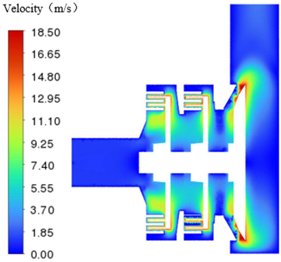
Figure 3.
Pump (M3) profile velocity distribution.
3.1.3. Shear Stress Analysis of Turntables
Driven by the rotor, the fluid gradually moves from the center to the edge. When the polymer passes through the gap between the stator and the rotor, it is squeezed, stretched, and ground under the action of dynamic pressure and shear force. Figure 4 shows the shear force distribution of the rotor in the grinding-type hybrid pump (M3). According to the distribution contour plot, high shear force areas are mainly concentrated at the tooth ends on the outer edge of the rotor in each transmission region.

Figure 4.
Pump (M3) rotor shear force distribution.
3.1.4. Polymer Distribution
Figure 5 and Figure 6 illustrate the viscosity and volume fraction distributions at sections A and D of the grinding-type hybrid pump (M3), respectively. As shown in the figures, the fluid volume fraction gradually decreases from the inlet to the outlet, while the fluid viscosity exhibits an opposite trend. The volume fraction of the polymer is highest at the inlet. After being squeezed, ground, and mixed by the gear structure, the polymer distribution within the cavity becomes relatively uniform, concentrating between 7.13 × 10⁻³, which is also reflected in the viscosity distribution chart of section D.

Figure 5.
Viscosity distribution of pump (M3) cross section (A,B).
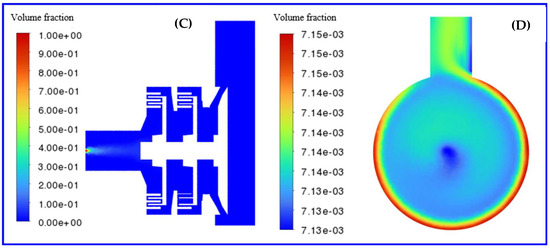
Figure 6.
Pump (M3) cross section (C,D) volume fraction distribution diagram.
Through the analysis of pressure distribution, fluid velocity, fluid viscosity, and volume fraction, it can be seen that the grinding-type hybrid pump (M3) has a certain effect on the grinding and dispersion of polymers. According to the working principle of the grinding-type hybrid pump, structural parameters have a significant impact on the grinding and mixing effect of polymers. Therefore, the number of stages, pump diameter, and number of teeth of the grinding-type hybrid pump will be optimized to improve the uniformity of the polymer blend solution.
3.2. Analysis of the Effect of Grinding Mixing Pump Stage (M1, M2, M3)
Figure 7 presents the structural models of the grinding-type hybrid pumps M1, M2, and M3. The main difference between them lies in the number of stages in the gear structure, meaning that the polymers undergo one-stage, two-stage, and three-stage grinding in pumps M1, M2, and M3, respectively. The following is a comparative analysis of the pressure, velocity, viscosity, and volume fraction within each stage of the grinding-type hybrid pumps.
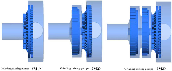
Figure 7.
Structural model of grinding mixing pumps (M1, M2, M3).
3.2.1. Pressure Profile Analysis
Figure 8 shows the pressure distribution profiles of the grinding-type hybrid pumps M1, M2, and M3. According to the pressure distribution contour plots, as the number of stages in the grinding-type hybrid pump increases, the inlet pressure gradually rises, with values of 1.74 × 10⁵ Pa for M1, 5.73 × 10⁵ Pa for M2, and 8.10 × 10⁵ Pa for M3. Moreover, the main pressure drop occurs in the gear structure for all three pumps, M1, M2, and M3, while the pressure changes in the channel structure and cavity structure are not significant.
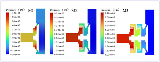
Figure 8.
Pump (M1, M2, M3) profile pressure distribution.
3.2.2. Velocity Profile Analysis
Figure 9 presents the velocity distribution profiles of the grinding-type hybrid pumps M1, M2, and M3. According to the velocity distribution contour plots, the main high-speed flow areas in all three pumps, M1, M2, and M3, are located in the gear structure, while the velocity changes in the channel structure and cavity structure are relatively small. Since the highest velocity is generated by the rotor’s transmission of fluid within the pump body in the gear structure, and the rotor speed and radius are equal in pumps M1, M2, and M3, the variation in the number of stages in the grinding-type hybrid pump has a minor impact on the maximum velocity of the fluid within the pump.
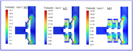
Figure 9.
Pump (M1, M2, M3) profile velocity distribution.
3.2.3. Polymer Distribution
- ①
- Viscosity distribution
Figure 10 and Figure 11 illustrate the cross-sectional viscosity distributions of the grinding mixing pumps M1, M2, and M3, as well as the viscosity distributions at various stages within each pump. As evident from the figures, the viscosity of the fluid within the grinding mixing pumps M1, M2, and M3 becomes increasingly uniform with the increase in pump stages. Specifically, the fluid viscosity differences within the chamber structures of pumps M1 and M2 are 1.93 kg/m·s and 0.16 kg/m·s, respectively, while the fluid viscosity within the chamber structure of pump M3 is almost uniform.
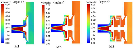
Figure 10.
Viscosity profile of pumps (M1, M2, M3).
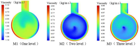
Figure 11.
Pump (M1, M2, M3) cross-sectional viscosity distribution diagram.
- ②
- Volume fraction distribution
Figure 12 and Figure 13 depict the cross-sectional volume fraction distributions of the grinding mixing pumps M1, M2, and M3, as well as the volume fraction distributions at various stages along each pump. As shown in the figures, the volume fraction of the fluid within the pump chambers also becomes increasingly uniform with an increase in the number of grinding passes. A further comparison is made of the volume fraction distributions along detection lines a, b, and at various stages. In the grinding mixing pumps M1, M2, and M3, the grinding and mixing effect of the polymers by the first-stage rotor–stator pair is insufficient, resulting in a significant span in the volume fraction distribution along the detection lines, as illustrated in Figure 14. Through further grinding by the second-stage rotor–stator pair, the volume fraction of the polymers in pumps M2 and M3 becomes relatively uniform. A comparative analysis of the volume fractions along the detection lines at various stages of the grinding mixing pumps reveals that pump M1 exhibits the poorest grinding and mixing effect on the polymers, with a volume fraction difference as high as 2.09 × 10⁻³. Although pump M2 improves the volume fraction of the polymers through the grinding of the second-stage rotor–stator, it still lags slightly behind pump M3 in terms of the uniformity of polymer distribution, as shown in Figure 15. Therefore, among the grinding mixing pumps M1, M2, and M3, the latter demonstrates the best grinding and mixing effect on the polymers.

Figure 12.
Pump (M1, M2, M3) profile volume fraction distribution.
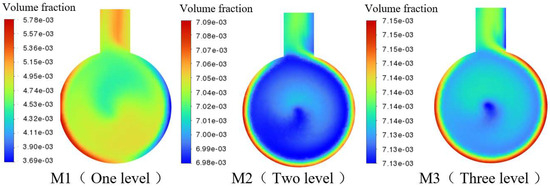
Figure 13.
Pump (M1, M2, M3) cross-sectional volume fraction distribution map at all levels.

Figure 14.
Pump (M1, M2, M3) detection line a volume fraction distribution curve.
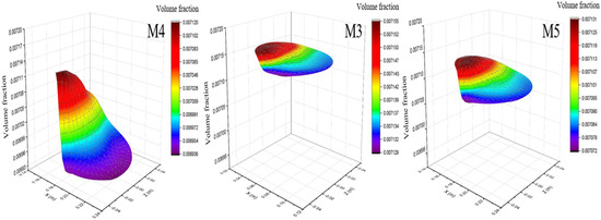
Figure 15.
Pump (M1, M2, M3) final section volume fraction distribution.
3.3. Diameter Effect Analysis of Grinding Mixing Pumps (M4, M3, M5)
Figure 16 presents the structural models of the grinding mixing pumps M4, M3, and M5. The main difference between them lies in their pump sizes. The grinding mixing pump M4 has the smallest pump diameter of 120 mm, while the grinding mixing pump M5 has the largest pump diameter of 160 mm. The size of the grinding mixing pump M3 falls between the two, with a pump diameter of 140 mm. Below, a comparative analysis of the pressure, velocity, viscosity, and volume fraction within these differently sized grinding mixing pumps is conducted.
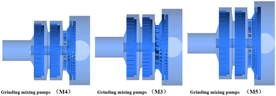
Figure 16.
Structural model of a grinding mixing pump (M4, M3, M5).
3.3.1. Pressure Profile Analysis
Figure 17 shows the cross-sectional pressure distributions of the grinding mixing pumps M4, M3, and M5. As can be seen from the pressure distribution contours, with the increase in the pump diameter of the grinding mixing pumps, the inlet pressure gradually decreases, reaching 9.94 × 10⁵ Pa for M4, 8.10 × 10⁵ Pa for M3, and 5.97 × 10⁵ Pa for M5. The main pressure drop occurs in the gear structure, while there is no significant change in pressure within the channel structure and chamber structure.
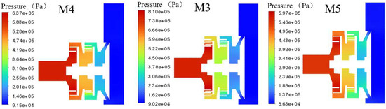
Figure 17.
Pump (M4, M3, M5) profile pressure distribution.
3.3.2. Velocity Profile Analysis
Figure 18 illustrates the cross-sectional velocity distributions of the grinding mixing pumps M4, M3, and M5. As can be seen from the velocity distribution contours, with the increase in the pump diameter of the grinding mixing pumps, the maximum velocity within the pump body gradually increases, reaching 17.27 m/s for M4, 18.50 m/s for M3, and 20.4 m/s for M5. Furthermore, the primary high-velocity flow regions in the grinding mixing pumps M4, M3, and M5 are all located within the gear structure, while the velocity changes within the channel structure and chamber structure are relatively small.

Figure 18.
Pump (M4, M3, M5) profile velocity distribution.
3.3.3. Polymer Distribution
- ①
- Viscosity distribution
Figure 19 and Figure 20 show the cross-sectional viscosity distributions and the viscosity distributions, respectively, at various stages of the grinding mixing pumps M4, M3, and M5. As can be seen from the figures, the viscosity of the fluid within the grinding mixing pumps M4, M3, and M5 exhibits a trend of first increasing and then decreasing as the pump diameter increases. The fluid viscosity at the three-stage section of the grinding mixing pump M4 ranges between 4.57 kg/m·s and 4.82 kg/m·s, indicating that further improvement in uniformity is needed. The fluid viscosity in the grinding mixing pump M3 is the most uniform, indicating that this pump has the best grinding and mixing effect on the polymers. The grinding mixing pump M5 has the largest size, and its uniformity falls between that of pumps M3 and M4.
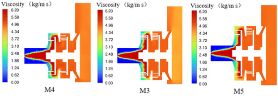
Figure 19.
Viscosity profile of pumps (M4, M3, M5).

Figure 20.
Viscosity profile of pumps (M4, M3, M5).
- ②
- Volume fraction distribution
Figure 21 and Figure 22 present the cross-sectional volume fraction distributions and the volume fraction distributions at various stages for the grinding-type mixing pumps M4, M3, and M5, respectively. The figures reveal that the volume fraction of the fluid within the pump cavity initially increases and then decreases as the pump diameter enlarges. A further comparison is made of the volume fraction distributions along detection lines a, b, and c. In grinding-type mixing pumps M4, M3, and M5, the grinding and mixing effectiveness of the polymers by the primary rotor–stator pairs all require improvement, as evidenced by the significant span in volume fraction distributions along detection line a, as shown in Figure 23. Following further grinding of the polymers by the secondary rotor–stator pair, the uniformity of polymer distribution in M4, which has a smaller pump diameter, is relatively poor, with volume fractions ranging between 7.04 × 10⁻³. Lastly, a comparative analysis of the volume fractions along detection line c and at the final stage cross-section for the grinding-type mixing pumps reveals that pumps M3 and M5 exhibit higher grinding and mixing effectiveness for the polymers, with greater uniformity, and average volume fractions of 7.14 × 10⁻³, as shown in Figure 24. Therefore, among the grinding-type mixing pumps M4, M3, and M5, pumps M3 and M5 demonstrate comparable grinding and mixing effectiveness for the polymers. Considering the manufacturing costs of the grinding-type mixing pumps, M3, with a relatively smaller pump diameter, is selected as the optimal structure.

Figure 21.
Pump (M4, M3, M5) profile volume fraction distribution.

Figure 22.
Section volume fraction distribution of pumps (M4, M3, M5) at all levels.

Figure 23.
Pump (M4, M3, M5) detection line c volume fraction distribution curve.

Figure 24.
Pump (M4, M3, M5) final section volume fraction distribution.
3.4. Analysis of the Effect of the Number of Teeth of the Grinding Mixing Pump (M3, M6)
Figure 25 illustrates the structural model of the grinding-type mixing pumps. The primary difference between the two lies in the number of teeth on the stator and rotor within their gear structures: the grinding-type mixing pump M3 features 60 teeth on both the stator and rotor, while the grinding-type mixing pump M6 has 45 teeth. Below is a comparative analysis of the pressure, velocity, viscosity, and volume fraction within these grinding-type mixing pumps of different sizes.
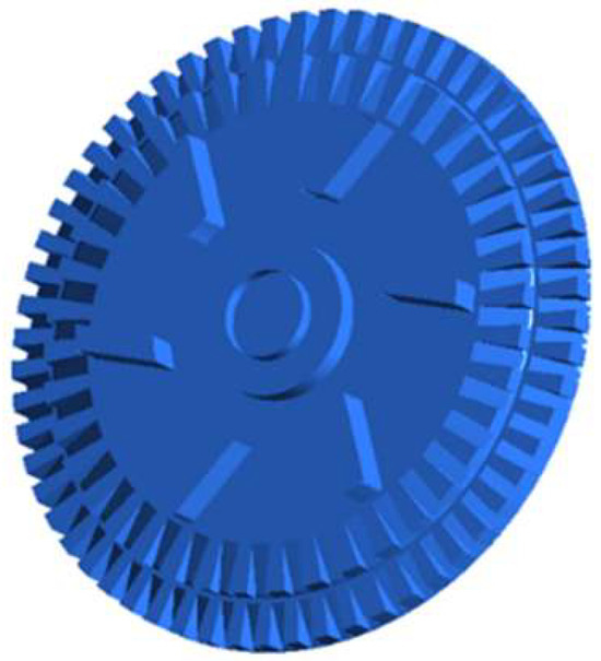
Figure 25.
Model diagram of the rotor structure of a grinding mixing pump.
3.4.1. Pressure Profile Analysis
Figure 26 shows the cross-sectional pressure distribution for the grinding-type mixing pumps M3 and M6. According to the pressure distribution contour plot, as the number of teeth in the gear structure of the grinding-type mixing pump decreases, the surface area of both the rotor and stator diminishes, leading to a reduction in the flow resistance experienced by the fluid. Consequently, the inlet pressure of pump M6 is lower compared to pump M3, measuring at 7.68 × 10⁵ (for M6). However, the primary pressure drop region for both pumps is within the gear structure, and there is insignificant pressure variation in the channel and cavity structures.
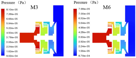
Figure 26.
Pump (M3, M6) profile pressure distribution.
3.4.2. Velocity Profile Analysis
Figure 27 displays the cross-sectional velocity distribution for the grinding-type mixing pumps M3 and M6. According to the velocity distribution contour plot, a reduction in the number of teeth on the rotor and stator within the gear structure of the grinding-type mixing pump facilitates an increase in fluid velocity within the pump body. The maximum fluid velocities within pumps M3 and M6 are 18.5 m/s and 19.7 m/s, respectively. Furthermore, the primary high-velocity flow regions for both pumps are within the gear structure, with relatively minor velocity variations observed within the channel and cavity structures.

Figure 27.
Pump (M3, M6) profile velocity distribution.
3.4.3. Polymer Distribution
- ①
- Viscosity distribution
Figure 28 and Figure 29 present the cross-sectional viscosity distributions and the viscosity distributions at various stages for the grinding-type mixing pumps M3 and M6, respectively. The figures indicate that changes in the number of teeth in the grinding-type mixing pump have a minor impact on viscosity but do affect its distribution uniformity. In the grinding-type mixing pump M6, the reduction in the number of teeth on the stator and rotor results in decreased stretching, grinding, and mixing of the polymers. At the third-stage cross-section, the fluid viscosity ranges between 4.54 kg/m·s and 4.82 kg/m·s, with a difference of 0.28 kg/m·s between the maximum and minimum values. In contrast, the difference in fluid viscosity at the third-stage cross-section of the grinding-type mixing pump M3 is only 0.03 kg/m·s. Therefore, the uniformity of the polymer solution in the grinding-type mixing pump M6 needs further improvement.
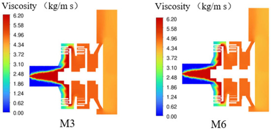
Figure 28.
Viscosity profile of pumps (M3, M6).
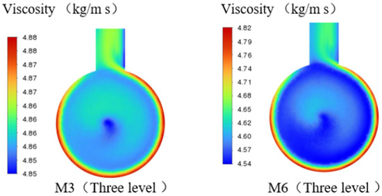
Figure 29.
Viscosity distribution diagram of pump (M3, M6) at all levels.
- ②
- Volume fraction distribution
Figure 30 and Figure 31 illustrate the cross-sectional volume fraction distributions and the volume fraction distributions at various stages for the grinding-type mixing pumps M3 and M6, respectively. The figures indicate that changes in the number of teeth on the stator and rotor in the grinding-type mixing pump have a significant impact on the uniformity of the volume fraction distribution.

Figure 30.
Pump (M3, M6) profile volume fraction distribution.
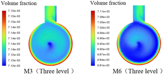
Figure 31.
Pump (M3, M6) section volume fraction distribution map.
A further comparison of the volume fraction distributions along detection lines a, b, and c is conducted. The polymer volume fraction along detection line a spans a wide range, indicating that in both grinding-type mixing pumps M3 and M6, the first-stage rotor–stator only performs initial grinding and mixing of the polymer. Although the second-stage rotor–stator further grinds the polymer, the volume fraction span along detection line b in pump M6 is reduced, mainly concentrating around 6.74 × 10⁻³. However, compared to grinding-type mixing pump M3, the uniformity of the polymer in M6 still needs improvement.
Finally, a comparative analysis of the volume fraction along detection line c and at the final stage cross-section in the grinding-type mixing pumps reveals that, due to the reduced number of teeth in the rotor–stator structure, the polymer volume fraction in pump M6 ultimately concentrates around 6.81 × 10⁻³, with poor uniformity, as shown in Figure 32 and Figure 33. In contrast, pump M3 exhibits higher grinding, mixing efficiency, and uniformity of the polymer. Therefore, M3, with a relatively higher number of teeth on the rotor–stator, is recommended as the optimal model for the grinding-type mixing pump.

Figure 32.
Pump (M3, M6) detection line c volume fraction distribution curve.

Figure 33.
Pump (M3, M6) final section volume fraction distribution.
4. Conclusions
Using Fluent software, CFD simulations were conducted on non-Newtonian fluids. Based on the simulated pressure profiles, velocity profiles, and polymer distributions, the number of stages, diameter, and number of teeth of the grinding pump were analyzed and optimized to obtain the optimal design of the device under the target conditions.
As the number of stages in the grinding-type mixing pump increases, the inlet pressure gradually increases. The main pressure drop occurs in the gear structure, while the pressure changes in the channel and cavity structures are not significant. The primary high-velocity flow regions are also located in the gear structure, with relatively minor velocity variations in the channel and cavity structures. According to the simulation results, both viscosity and volume fraction become more uniform with an increasing number of pump stages. In particular, the fluid viscosity in the cavity structure of pump M3 is almost uniform. A comparison of the volume fraction distributions at the outlet detection line and the outlet section of the grinding-type mixing pump under the same scale shows that the volume fraction of pump M3 is mainly concentrated around 7.12 × 10⁻³, with the most uniform distribution and the best grinding and mixing effect on the polymer.
The simulations also indicate that as the diameter of the mixing pump increases, the inlet pressure gradually decreases. The main pressure drop still occurs in the gear structure, and the maximum velocity within the pump body gradually increases. The high-velocity flow regions are consistently located in the gear structure. The viscosity and volume fraction of the fluid in the pump cavity initially increase and then decrease with the increase in pump diameter. The fluid viscosity in the third-stage cross-section of pump M4 ranges between 4.57 kg/m·s and 4.82 kg/m·s. Pump M3 exhibits the most uniform fluid viscosity, while pump M5’s uniformity is between those of M3 and M4. A comparison of the volume fraction distributions at the third-stage detection line and the outlet section of the grinding-type mixing pump under the same scale reveals that the volume fraction trends of pumps M3 and M5 are similar, with both showing high uniformity. However, pump M3 has the highest uniformity and the best grinding effect among the three.
With a decrease in the number of teeth in the gear structure of the grinding-type mixing pump, the surface area of the rotor and stator decreases, reducing the flow resistance experienced by the fluid. This results in a lower inlet pressure for pump M6 compared to pump M3, while also facilitating an increase in fluid velocity within the pump body. A comparison of the volume fraction distributions at the third-stage detection line and the outlet section of the grinding-type mixing pump under the same scale shows that pump M3 has both a higher volume fraction and a more uniform distribution, indicating the best grinding effect.
Author Contributions
Conceptualization, H.D.; methodology, C.W.; software, H.D.; validation, J.Z.; formal analysis, X.L.; investigation, X.Z.; resources, X.H.; data curation, X.W.; writing—original draft preparation, H.D.; writing—review and editing, C.W.; visualization, X.H.; supervision, J.Z.; project administration, X.L.; funding acquisition, J.Z. All authors have read and agreed to the published version of the manuscript.
Funding
This research received no external funding.
Data Availability Statement
Data are contained within the article.
Conflicts of Interest
Authors Hong Du, Chenxi Wang, Jian Zhang, Xianjie Li and Xiujun Wang were employed by the company CNOOC Research Institute Ltd. The remaining authors declare that the research was conducted in the absence of any commercial or financial relationships that could be construed as a potential conflict of interest.
References
- Wu, B. CFD Investigation of Turbulence Models for Mechanical Agitation of Non-Newtonian Fluids in Anaerobic Digesters. Water Res. 2011, 45, 2082–2094. [Google Scholar] [CrossRef]
- Rodríguez-Rivero, C.; Nogareda, J.; Martín, M.; del Valle, E.M.M.; Galán, M.A. CFD Modeling and Its Validation of Non-Newtonian Fluid Flow in a Microparticle Production Process Using Fan Jet Nozzles. Powder Technol. 2013, 246, 617–624. [Google Scholar] [CrossRef]
- Niazi, M.; Ashrafizadeh, S.N.; Hashemabadi, S.H.; Karami, H. CFD Simulation of Drag-Reducing Fluids in a Non-Newtonian Turbulent Pipe Flow. Chem. Eng. Sci. 2024, 285, 119612. [Google Scholar] [CrossRef]
- Rasouli, M.; Mousavi, S.M.; Azargoshasb, H.; Jamialahmadi, O.; Ajabshirchi, Y. CFD Simulation of Fluid Flow in a Novel Prototype Radial Mixed Plug-Flow Reactor. J. Ind. Eng. Chem. 2018, 64, 124–133. [Google Scholar] [CrossRef]
- Sorgun, M.; Ulker, E.; Uysal, S.O.K.; Muftuoglu, T.D. CFD Modeling of Turbulent Flow for Non-Newtonian Fluids in Rough Pipes. Ocean Eng. 2022, 247, 110777. [Google Scholar] [CrossRef]
- Ershadnia, R.; Amooie, M.A.; Shams, R.; Hajirezaie, S.; Liu, Y.; Jamshidi, S.; Soltanian, M.R. Non-Newtonian Fluid Flow Dynamics in Rotating Annular Media: Physics-Based and Data-Driven Modeling. J. Pet. Sci. Eng. 2020, 185, 106641. [Google Scholar] [CrossRef]
- Li, B.; Huang, C.; Liu, L.Y.; Yao, L.; Ning, B.; Yang, L. Separation Efficiency Prediction of Non-Newtonian Oil-Water Swirl-Vane Separators in Offshore Platform Based on GA-BP Neural Network. Ocean Eng. 2024, 296, 116984. [Google Scholar] [CrossRef]
- Bridgeman, J. Computational Fluid Dynamics Modelling of Sewage Sludge Mixing in an Anaerobic Digester. Adv. Eng. Softw. 2012, 44, 54–62. [Google Scholar] [CrossRef]
- Sadeghi, M.; Sontti, S.G.; Zheng, E.; Zhang, X. Computational Fluid Dynamics (CFD) Simulation of Three–Phase Non–Newtonian Slurry Flows in Industrial Horizontal Pipelines. Chem. Eng. Sci. 2023, 270, 118513. [Google Scholar] [CrossRef]
- Valdés, J.P.; Becerra, D.; Rozo, D.; Cediel, A.; Torres, F.; Asuaje, M.; Ratkovich, N. Comparative Analysis of an Electrical Submersible Pump’s Performance Handling Viscous Newtonian and Non-Newtonian Fluids through Experimental and CFD Approaches. J. Pet. Sci. Eng. 2020, 187, 106749. [Google Scholar] [CrossRef]
- Aldi, N.; Buratto, C.; Casari, N.; Dainese, D.; Mazzanti, V.; Mollica, F.; Munari, E.; Occari, M.; Pinelli, M.; Randi, S.; et al. Experimental and Numerical Analysis of a Non-Newtonian Fluids Processing Pump. Energy Procedia 2017, 126, 762–769. [Google Scholar] [CrossRef]
- Gu, D.; Xu, H.; Ye, M.; Wen, L. Design of Impeller Blades for Intensification on Fluid Mixing Process in a Stirred Tank. J. Taiwan Inst. Chem. Eng. 2022, 138, 104475. [Google Scholar] [CrossRef]
- Amani, E.; Ahmadpour, A.; Aghajari, M.J. Large-Eddy Simulation of Turbulent Non-Newtonian Flows: A Comparison with State-of-the-Art RANS Closures. Int. J. Heat Fluid Flow 2023, 99, 109076. [Google Scholar] [CrossRef]
- Heydari, O.; Sahraei, E.; Skalle, P. Investigating the Impact of Drillpipe’s Rotation and Eccentricity on Cuttings Transport Phenomenon in Various Horizontal Annuluses Using Computational Fluid Dynamics (CFD). J. Pet. Sci. Eng. 2017, 156, 801–813. [Google Scholar] [CrossRef]
- Ramírez-Muñoz, J.; Márquez-Baños, V.E.; Alvarez-Vega, J.; Mompremier, R.; Núñez, J.G.; Guadarrama-Pérez, R. Hydrodynamics Performance of Newtonian and Shear-Thinning Fluids in a Tank Stirred with a High Shear Impeller: Effect of Liquid Height and off-Bottom Clearance. Chem. Eng. Res. Des. 2023, 192, 44–54. [Google Scholar] [CrossRef]
- Chen, L.; Yang, Y.; Song, X.; Zhang, X.; Gong, Y.; Peng, C. Study on the Influence of Non-Newtonian Fluid Characteristics on the Hydraulic Performance and Internal Flow Field of Multiphase Pump. Chem. Eng. Res. Des. 2024, 202, 178–190. [Google Scholar] [CrossRef]
- Dyck, N.J.; Parker, M.J.; Straatman, A.G. The Impact of Boundary Treatment and Turbulence Model on CFD Simulations of the Ranque-Hilsch Vortex Tube. Int. J. Refrig. 2022, 141, 158–172. [Google Scholar] [CrossRef]
- Singh, J.P.; Kumar, S.; Mohapatra, S.K. Modelling of Two Phase Solid-Liquid Flow in Horizontal Pipe Using Computational Fluid Dynamics Technique. Int. J. Hydrogen Energy 2017, 42, 20133–20137. [Google Scholar] [CrossRef]
- Lilibeth, N.; Ricardo, G.; Jannike, S. Viscous effects on gas-liquid hydrodynamics for bubble size determinations in different Newtonian and non-Newtonian fluids using a CFD-PBM model. Chem. Eng. Sci. 2023, 282, 119324. [Google Scholar] [CrossRef]
- Nirmalkar, N.; Chhabra, R.P.; Poole, R.J. On creeping flow of a Bingham plastic fluid past a square cylinder. J. Non-Newton. Fluid Mech. 2012, 171, 17–30. [Google Scholar] [CrossRef]
- Divya, B.B.; Manjunatha, G.; Rajashekhar, C.; Vaidya, H.; Prasad, K.V. Analysis of temperature dependent properties of a peristaltic MHD flow in a non-uniform channel: A Casson fluid model. Ain Shams Eng. J. 2021, 12, 2181–2191. [Google Scholar] [CrossRef]
Disclaimer/Publisher’s Note: The statements, opinions and data contained in all publications are solely those of the individual author(s) and contributor(s) and not of MDPI and/or the editor(s). MDPI and/or the editor(s) disclaim responsibility for any injury to people or property resulting from any ideas, methods, instructions or products referred to in the content. |
© 2025 by the authors. Licensee MDPI, Basel, Switzerland. This article is an open access article distributed under the terms and conditions of the Creative Commons Attribution (CC BY) license (https://creativecommons.org/licenses/by/4.0/).