Application of Mathematical Modelling to Reducing and Minimising Energy Requirement for Oxygen Transfer in Batch Stirred Tank Bioreactors

Abstract
:1. Introduction
- Air compressor power requirement
- Agitator power requirement
2. Mathematical Modelling
2.1. Bioprocess Kinetics and Oxygen Uptake
2.2. Oxygen Transfer and Agitator Mechanical Power
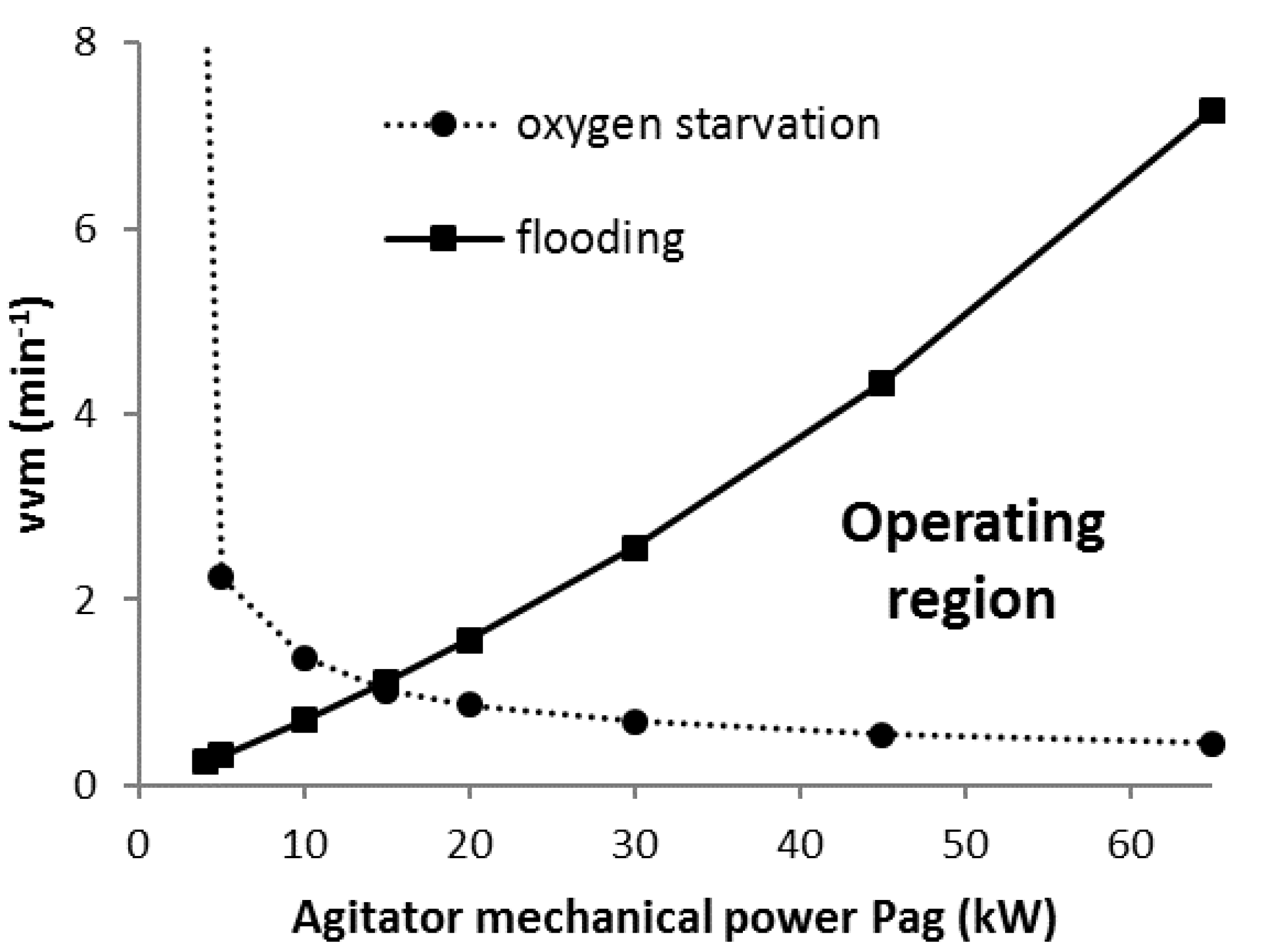
2.3. Flooding and Phase Equilibrium Constraints
2.4. Aeration System Energy Requirement
2.5. Modelling Scenarios
- Scenario K: Both Pag and vvm are maintained as constant. This may occur in some bioprocesses which are operated under fixed conditions of agitator power input and air flowrate.
- Scenario C: The oxygen concentration in the liquid is kept constant throughout the bioprocess. This represents a practical control strategy by monitoring oxygen concentration in the liquid and controlling either agitator power input or air flowrate or both to maintain the oxygen concentration at a constant value. This was implemented for the following sub-scenarios:
- Scenario C1: Pag is kept constant throughout the bioprocess and vvm is varied. From an oxygen transfer energy perspective, it is later shown that dividing the bioprocess time up into two or more time segments with different constant Pag values and varying vvm in each time segment significant energy savings may be obtained (this is referred to as Scenario C1-N, where N is the number of time segments).
- Scenario C2: vvm is kept constant and Pag is varied.
- Scenario C3 and Cmin: Scenario C3 is where both Pag and vvm are varied. It will be shown later that a Pag-vvm combination profile over time can be evaluated that minimises the total electrical energy required for a specified constant oxygen concentration in the liquid. This is referred to as scenario Cmin.
2.6. Model Implementation
3. Results and Discussion
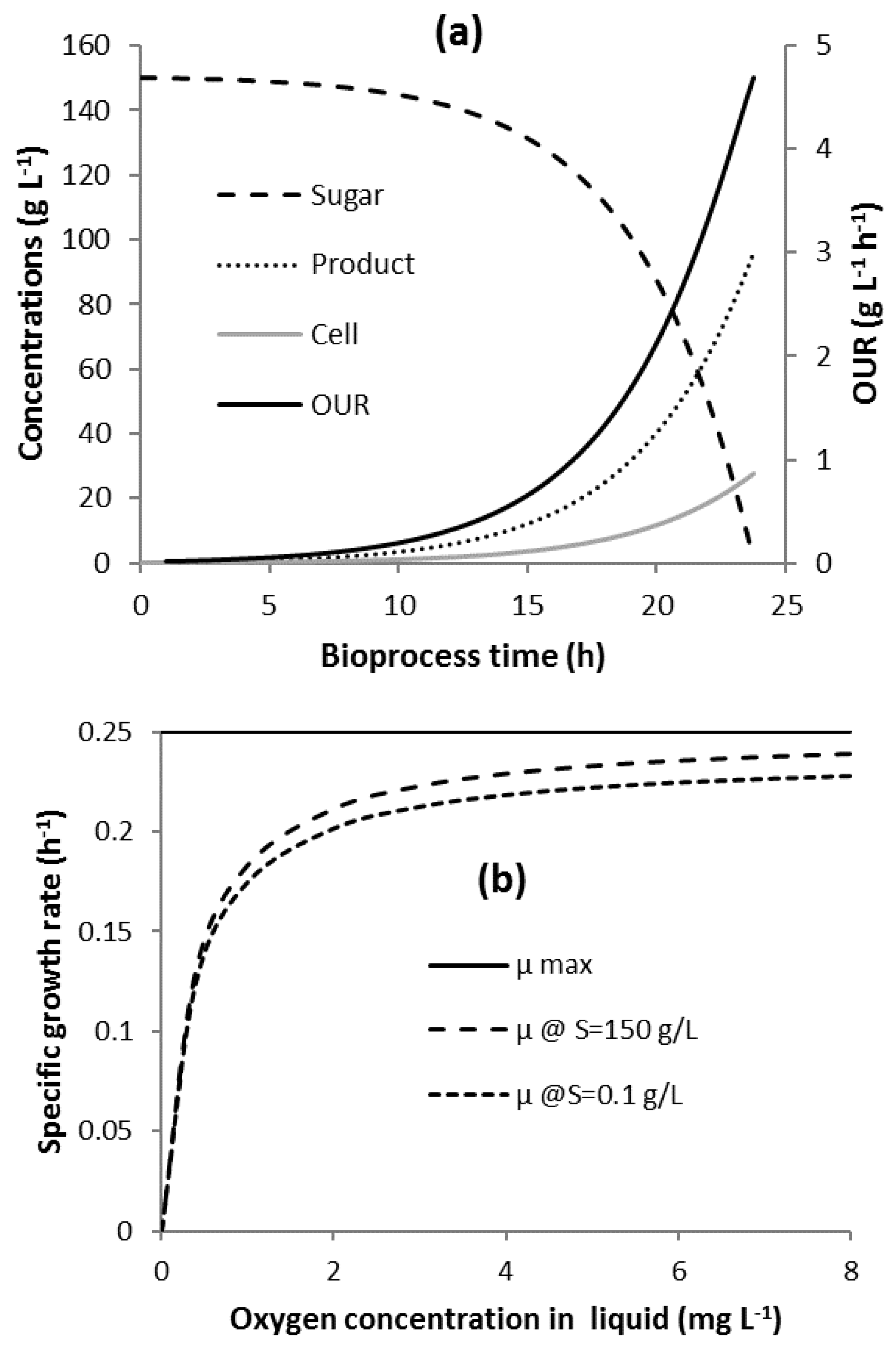
3.1. Bioprocess Progression
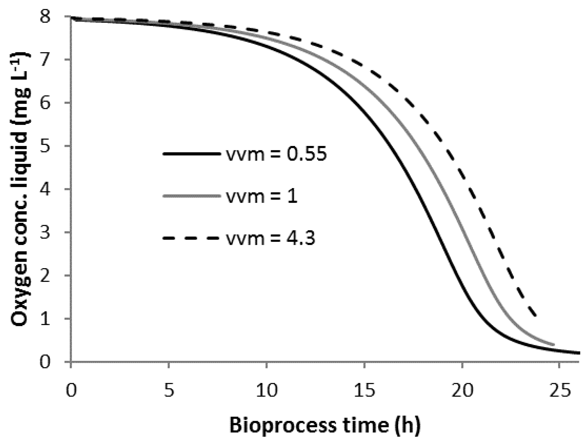
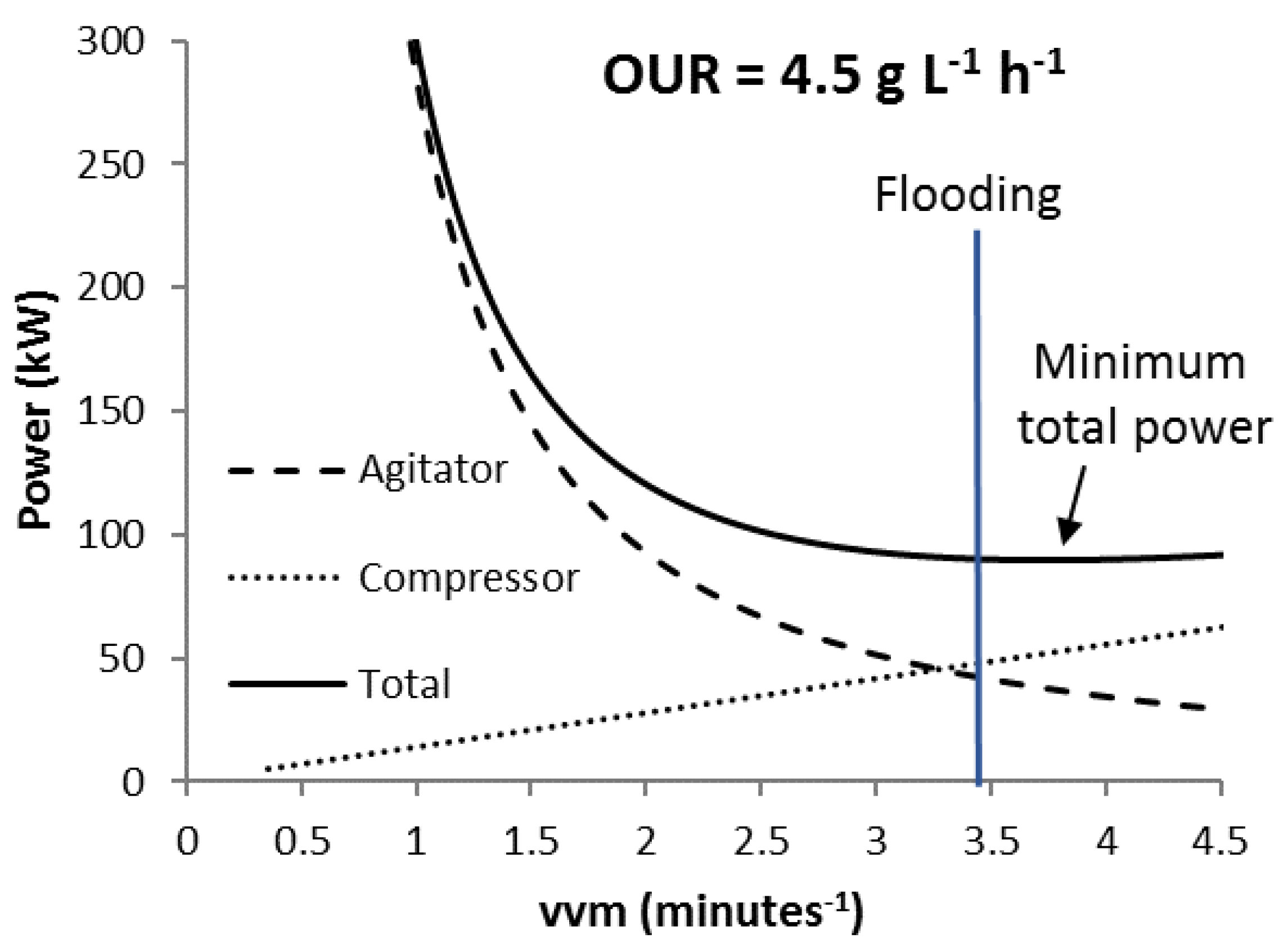
3.2. Scenario K
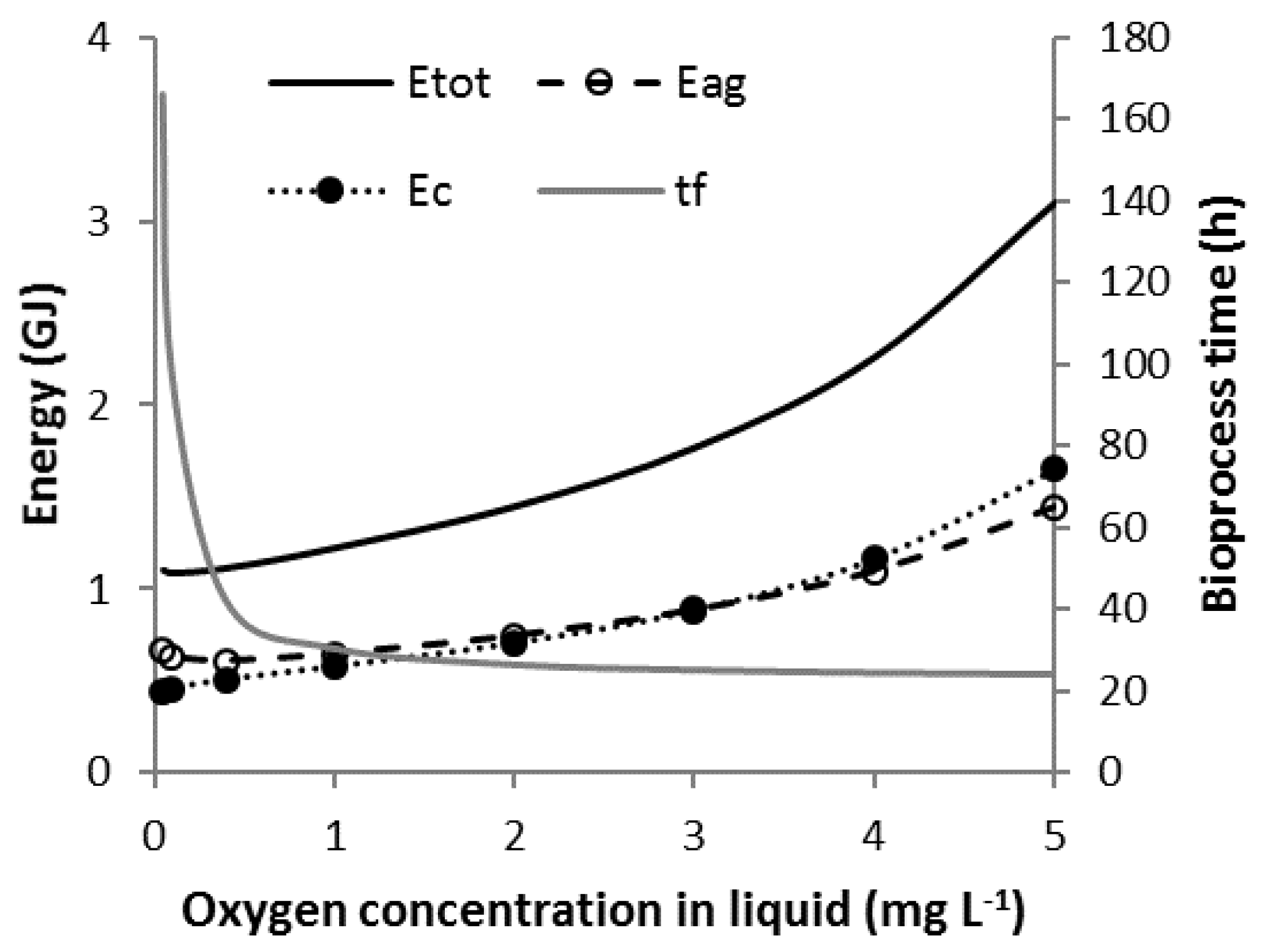
3.3. Scenario C
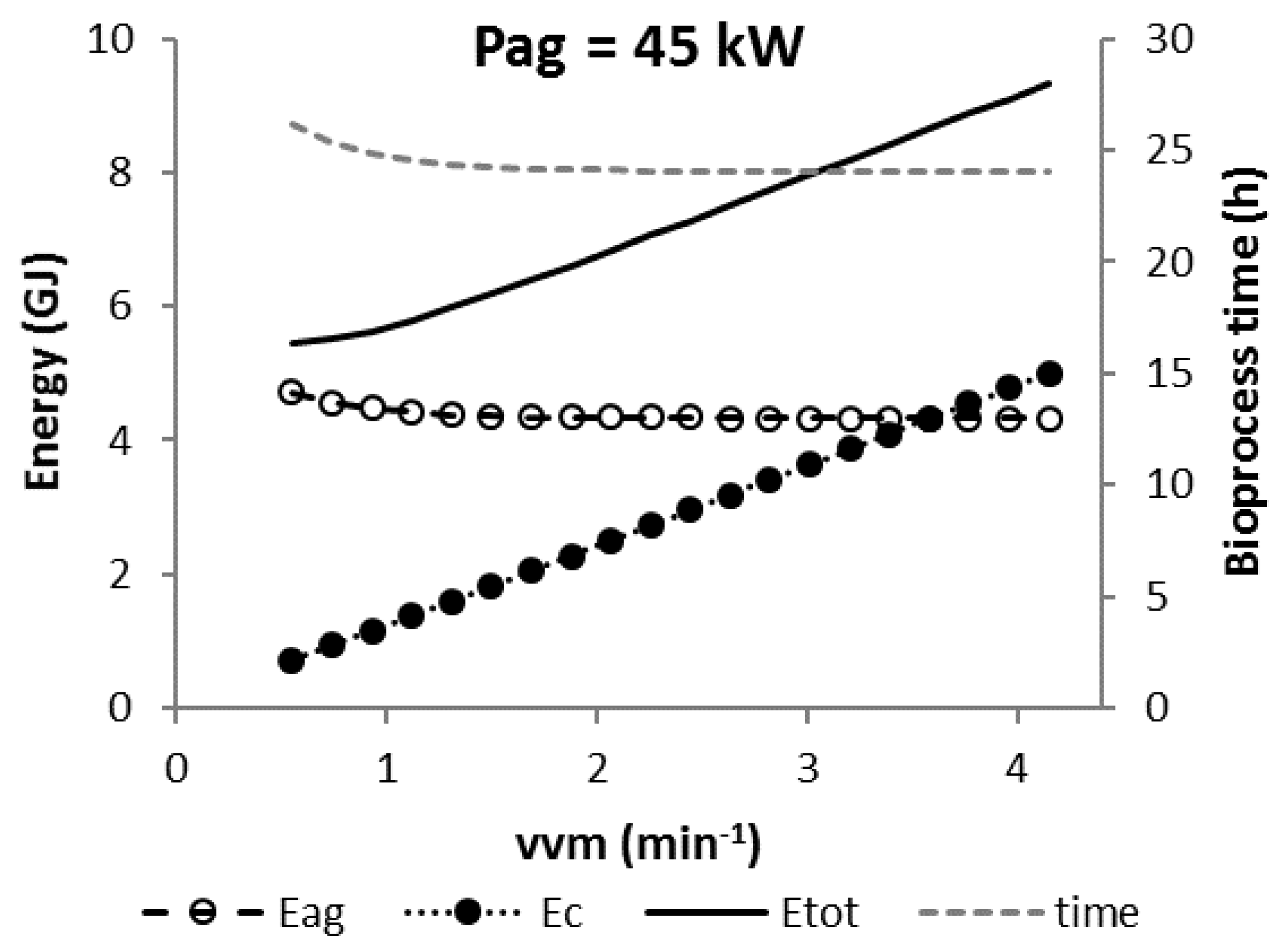
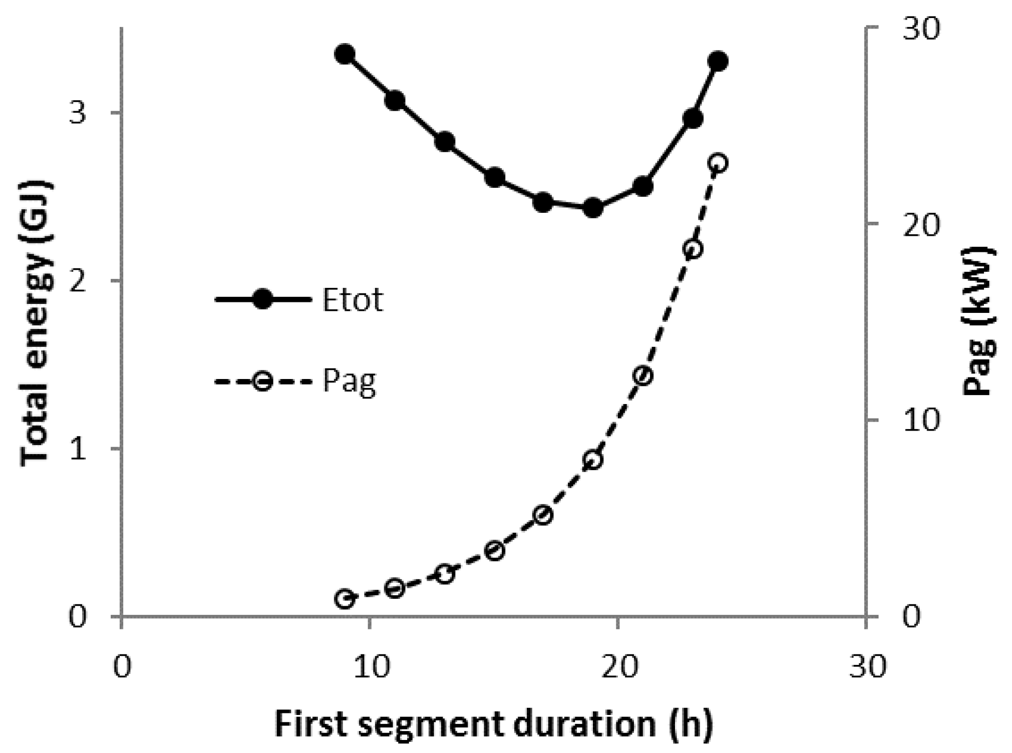
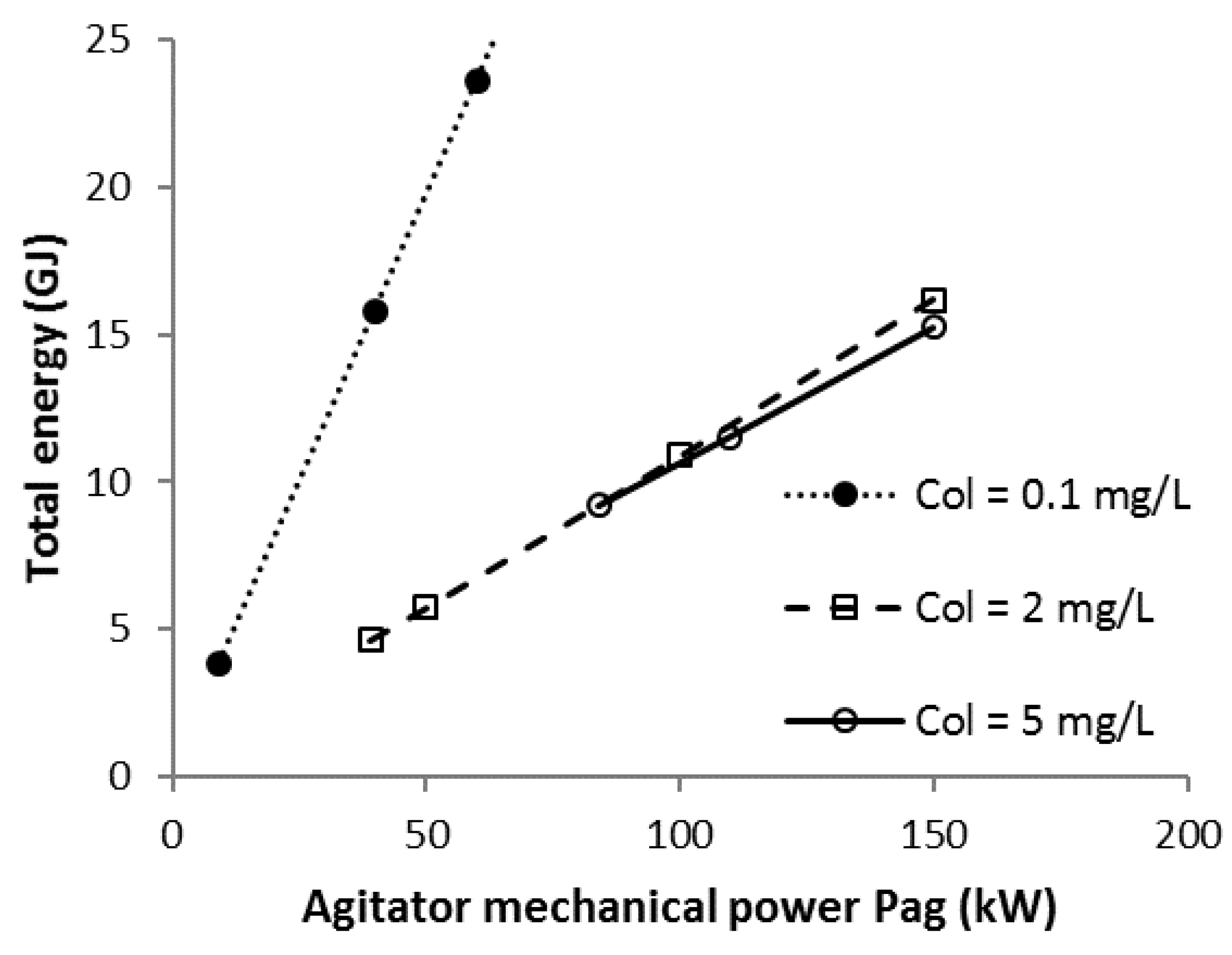
3.4. Scenario C1
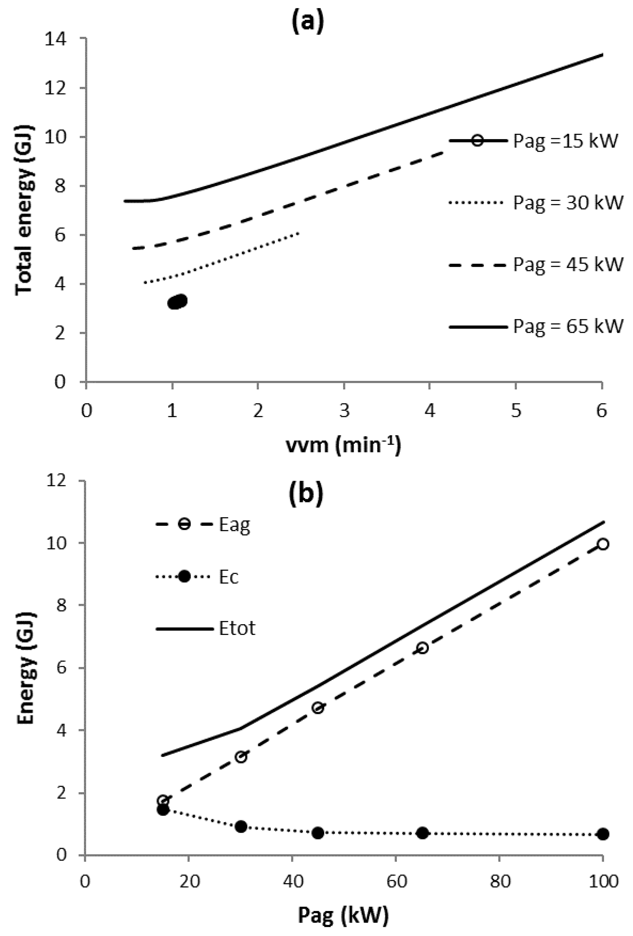
3.5. Scenario C2
3.6. Scenario C3
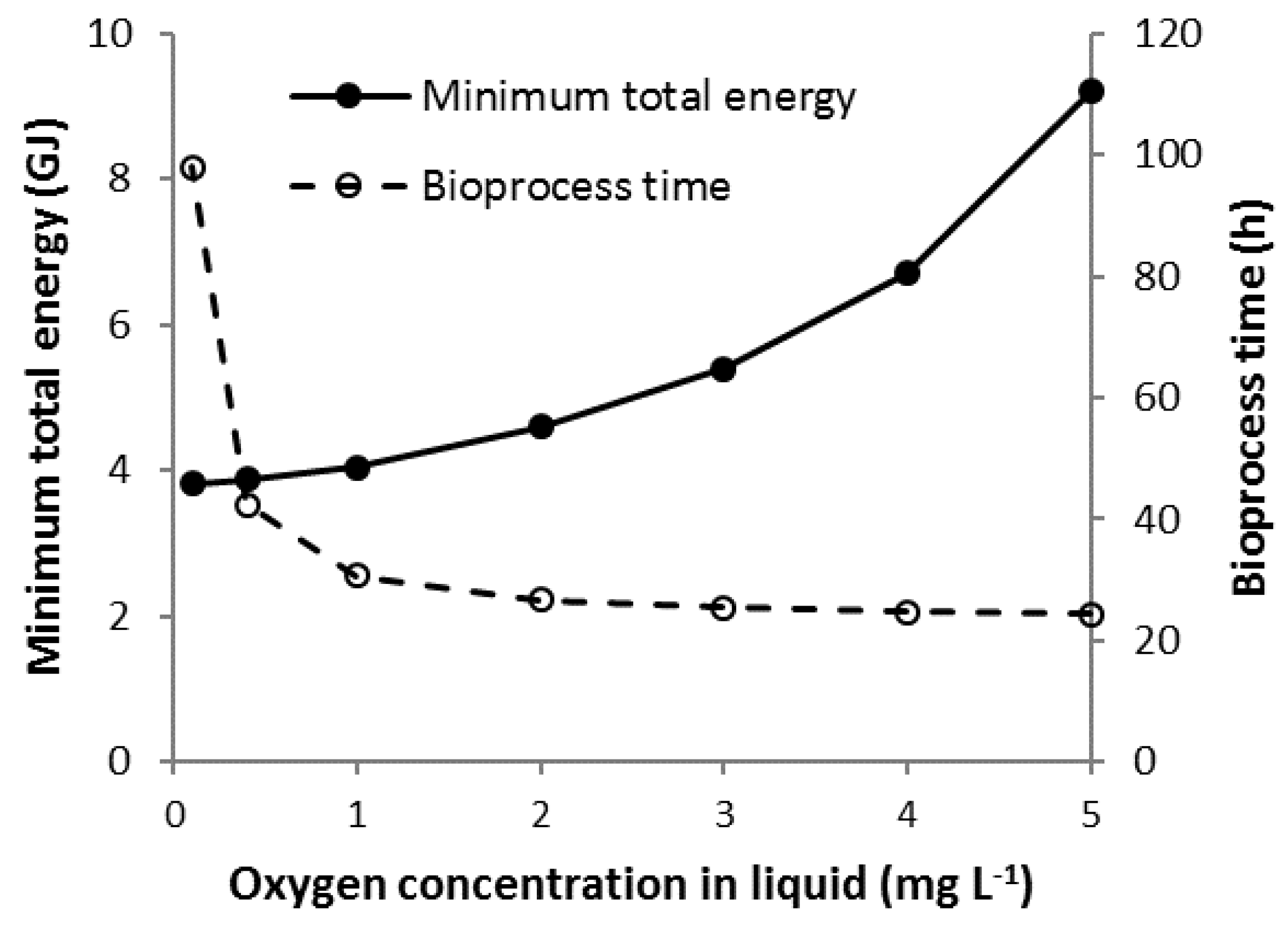
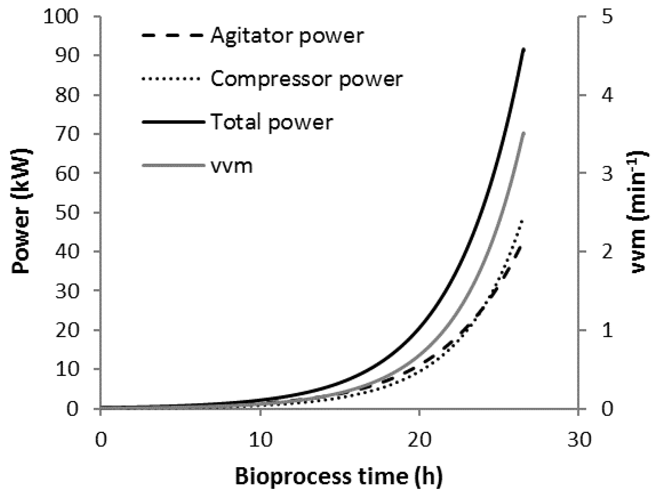
3.7. Scenario Cmin
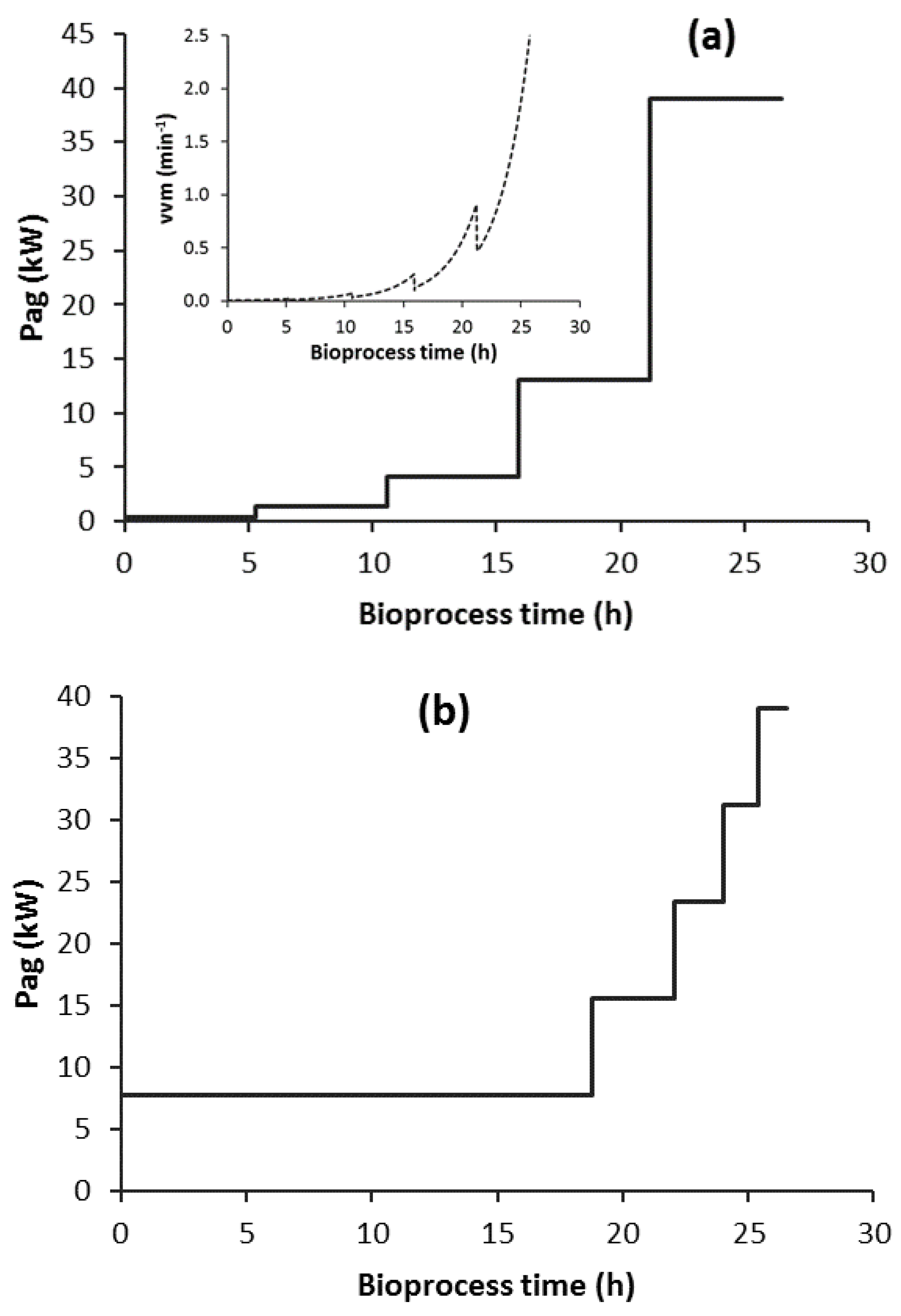
3.8. Scenario C1-N
3.9. Comparison of Scenario Minimum Total Energy Requirements
4. Conclusions
Author Contributions
Funding
Conflicts of Interest
List of Symbols
| AT | cross-sectional area of bioreactor (m2) |
| COG | oxygen concentration in air bubble (mg·L−1) |
| COGI | oxygen concentration in air entering bioreactor (mg·L−1) |
| COGO | oxygen concentration in air leaving bioreactor (mg·L−1) |
| COL | oxygen concentration in the bioprocess broth (mg·L−1) |
| D | impeller diameter (m) |
| Eag | agitator electrical energy (GJ) |
| Ec | compressor electrical energy (GJ) |
| Etot | sum of agitator and compressor electrical energy (GJ) |
| FG | inlet air volumetric flowrate (m3·h−1) |
| kLa | volumetric oxygen mass transfer coefficient (h−1) |
| KO | Monod kinetic constant for oxygen (g·L−1) |
| KR | Monod kinetic constant (g·L−1) |
| KS | Monod kinetic constant for sugar (g·L−1) |
| M | Henry’s Law constant |
| mS | specific maintenance coefficient (h−1) |
| N | agitator rotational speed (s−1) |
| NA | aeration number |
| NFr | Froude number |
| NP | agitator power number (ungassed) |
| NPG | agitator power number (gassed) |
| OUR | oxygen uptake rate (g·L−1·h−1) |
| OTR | oxygen transfer rate (g·L−1·h−1) |
| P | production concentration (g·L−1) |
| Pag | agitator mechanical power input (kW) |
| Patm | atmospheric pressure (Pa) |
| PC | compressor mechanical power input (kW) |
| Pi | atmospheric pressure + static head in bioreactor (Pa) |
| S | sugar concentration (g·L−1) |
| SR | rate-limiting substrate concentration (g·L−1) |
| t | time (h) |
| tf | bioprocess time (h) |
| T | bioreactor diameter (m) |
| VL | bioreactor working volume (m−3) |
| vvm | volume of air per minute per unit bioreactor working volume (min−1) |
| vs | air superficial velocity (m·h−1) |
| X | cell concentration (g·L−1) |
| YXS | yield coefficient for biomass (g dry cell weight per g sugar) |
| YPS | yield coefficient for product (g product per g sugar) |
| α, β | product production rate model constants |
| δ, Φ | OUR model constants |
| µ | specific growth rate (h−1) |
| µmax | maximum specific growth rate (h−1) |
| γ | isentropic exponent of compression |
References
- Garcia-Ochoa, F.; Gomez, E. Bioreactor scale-up and oxygen transfer rate in microbial processes: An overview. Biotechnol. Adv. 2009, 27, 153–176. [Google Scholar] [CrossRef] [PubMed]
- Bartholomew, W.H.; Karow, E.O.; Sfat, M.R. Oxygen transfer and agitation in submerged fermentations mass transfer of oxygen in submerged fermentation of Streptomyces griseus. Ind. Eng. Chem. 1950, 42, 1801–1809. [Google Scholar] [CrossRef]
- Bartholomew, W.H.; Karow, E.O.; Sfat, M.R.; Wilhelm, R.H. Effect of air flow and agitation rates upon fermentation of Penicillium chrysogenum and Streptomyces griseus. Ind. Eng. Chem. 1950, 42, 1810–1815. [Google Scholar] [CrossRef]
- Juarez, P.; Orejas, J. Oxygen transfer in a stirred reactor in laboratory scale. Lat. Am. Appl. Res. 2001, 31, 433–439. [Google Scholar]
- Demirtas, M.U.; Kolhatkar, A.; Kilbane, J.J. Effect of aeration and agitation on growth rate of Thermus thermophilus in batch mode. J. Biosci. Bioeng. 2003, 95, 113–117. [Google Scholar] [CrossRef]
- Bandaiphet, C.; Prasertsan, P. Effect of aeration and agitation rates and scale-up on oxygen transfer coefficient, kLa in exopolysaccharide production from Enterobacter cloacae WD7. Carbohydr. Polym. 2006, 66, 216–228. [Google Scholar] [CrossRef]
- Huang, W.C.; Chen, S.J.; Chen, T.L. The role of dissolved oxygen and function of agitation in hyaluronic acid fermentation. Biochem. Eng. J. 2006, 32, 239–243. [Google Scholar] [CrossRef]
- Radchenkovaa, N.; Vassilev, S.; Martinov, M.; Kuncheva, M.; Panchev, I.; Vlaev, S.; Kambourova, M. Optimization of the aeration and agitation speed of Aeribacillus palidus418 exopolysaccharide production and the emulsifying properties of the product. Process Biochem. 2014, 49, 576–582. [Google Scholar] [CrossRef]
- Kouda, T.; Yano, H.; Yoshinaga, F. Effect of agitator configuration on bacterial cellulose productivity in aerated and agitated culture. J. Ferment. Bioeng. 1997, 83, 371–376. [Google Scholar] [CrossRef]
- Amanullah, A.; Tuttiett, B.; Nienow, A.W. Agitator speed and dissolved oxygen effects in xanthan fermentations. Biotechnol. Bioeng. 1998, 57, 198–210. [Google Scholar] [CrossRef]
- Karimi, A.; Golbabaei, F.; Reza Mehrnia, M.; Neghab, M.; Kazem, M.; Nikpey, A.; Reza Pourmand, M. Oxygen mass transfer in a stirred tank bioreactor using different impeller configurations for environmental purposes. J. Environ. Health Sci. Eng. 2013, 10, 1–9. [Google Scholar] [CrossRef] [PubMed]
- Benz, G.T. Sizing impellers for agitated aerobic fermenters. Chem. Eng. Prog. 2004, 100, 18S–20S. [Google Scholar]
- Himmelsbach, W.; Keller, W.; Lovallo, M.; Grebe, T.; Houlton, D. Increase Productivity through better gas-liquid mixing. Chem. Eng. 2007, 10, 50–58. [Google Scholar]
- Bakker, A.; Smith, J.M.; Meyers, K.J. How to disperse gases in liquids. Chem. Eng. 1994, 12, 98–104. [Google Scholar]
- Hixson, A.W.; Caden, L.E., Jr. Oxygen transfer in submerged fermentation. Ind. Eng. Chem. 1950, 42, 1793–1800. [Google Scholar] [CrossRef]
- Badino, A.C.; De Almeida, P.I.F.; Cruz, A.J.G. Agitation and aeration an automated didactic experiment. Chem. Eng. Educ. 2004, 38, 100–107. [Google Scholar]
- Fayolle, Y.; Cockx, A.; Gillot, S.; Roustan, M.; Héduit, A. Oxygen transfer prediction in aeration tanks using CFD. Chem. Eng. Sci. 2007, 62, 7163–7171. [Google Scholar] [CrossRef]
- Gill, N.K.; Appleton, M.; Baganz, F.; Lye, G.J. Quantification of power consumption and oxygen transfer characteristics of a stirred miniature bioreactor for predictive fermentation scale-up. Biotechnol. Bioeng. 2008, 100, 1144–1155. [Google Scholar] [CrossRef]
- Benz, G.T. Piloting bioreactors for agitation scale-up. Chem. Eng. Prog. 2008, 104, 32–34. [Google Scholar]
- Benz, G.T. Why conduct pilot studies for agitated gas-liquid mass transfer. Pharm. Eng. 2013, 33, 1–3. [Google Scholar]
- Alves, S.S.; Vasconcelos, J.M.T. Optimisation of agitation and aeration in fermenters. Bioprocess Eng. 1996, 14, 119–123. [Google Scholar] [CrossRef]
- Benz, G.T. Optimize power consumption in aerobic fermenters. Chem. Eng. Prog. 2003, 99, 32–35. [Google Scholar]
- Benz, G.T. Cut agitator power costs. Chem. Eng. Prog. 2012, 108, 40–43. [Google Scholar]
- Zamouche, R.; Bencheikh-Lehocine, M.; Meniai, A.H. Oxygen transfer and energy savings in a pilot-scale batch reactor for domestic wastewater treatment. Desalination 2007, 206, 414–423. [Google Scholar] [CrossRef]
- Oliveira, R.; Simutis, R.; Feyo de Azevedo, S. Design of a stable adaptive controller for driving aerobic fermentation processes near maximum oxygen transfer capacity. J. Process Control 2004, 14, 617–626. [Google Scholar] [CrossRef]
- Kreyenschulte, D.; Emde, F.; Regestein, L.; Büch, J. Computational minimization of the specific energy demand of large-scale aerobic fermentation processes based on small-scale data. Chem. Eng. Sci. 2016, 153, 270–283. [Google Scholar] [CrossRef]
- van’t Riet, K.; Tramper, H. Basic Bioreactor Design; Marcel Dekker Inc.: New York, NY, USA, 1991. [Google Scholar]
- Znad, H.; Blazej, M.; Bales, V.; Markos, J. A kinetic model for gluconic acid production by Aspergillus niger. Chem. Pap. 2004, 58, 23–28. [Google Scholar]
- Liu, J.Z.; Weng, L.; Zhang, Q.; Xu, H.; Ji, L. A mathematical model for gluconic acid fermentation by Aspergillus Niger. Biochem. Eng. J. 2003, 14, 137–141. [Google Scholar] [CrossRef]
- Crueger, W.; Crueger, A. Biotechnology: A Textbook of Industrial Microbiology; Sinauer Associates: Sunderland, MA, USA, 1982. [Google Scholar]
- Merchuk, J.C.; Asenjo, J.A. The Monod equation and mass transfer. Biotech. Bioeng. 1995, 45, 973–980. [Google Scholar] [CrossRef]
- Beyenal, H.; Chen, S.N.; Lewandowski, Z. The double substrate growth kinetics of Pseudomonas aeruginosa. Enzym. Microb. Technol. 2003, 32, 92–98. [Google Scholar] [CrossRef]
- Slininger, P.J.; Branstrator, L.E.; Bothast, R.J.; Okost, M.R.; Ladisch, M.R. Growth, Death, and Oxygen Uptake Kinetics of Pichia stipitis on Xylose. Biotechnol. Bioeng. 1991, 37, 973–980. [Google Scholar] [CrossRef] [PubMed]
- Garcia-Ochoa, F.; Gomez, E.; Santos, V.E.; Merchuk, J.C. Oxygen uptake rate in microbial processes: An overview. Biochem. Eng. J. 2010, 49, 289–307. [Google Scholar] [CrossRef]
- van’t Riet, K. Review of measuring methods and results in non-viscous gas-liquid mass transfer in stirred vessels. Ind. Eng. Chem. Process Des. Dev. 1979, 18, 357–364. [Google Scholar] [CrossRef]


| μmax (h−1) | KS (g·L−1) | KO (g·L−1) | α | β (h−1) | YXS | YPS | mS (h−1) |
|---|---|---|---|---|---|---|---|
| 0.25 | 0.005 | 0.000363 | 2.9220 | 0.1314 | 0.55 | 1 | 0.025 |
| kLa Correlations and References | Constants | ||
|---|---|---|---|
| K | n1 | n2 | |
| 1—van’t Riet non-coalesce [van’t Riet, 1979] | 0.026 | 0.4 | 0.5 |
| 2—van’t Riet coalesce [van’t Riet, 1979] | 0.002 | 0.7 | 0.2 |
| 3—Benz broth 1 [Benz, 2013] | 0.015 | 0.55 | 0.6 |
| 4—Benz broth 2 [Benz, 2013] | 0.088 | 0.542 | 0.741 |
| 5—Bakker [Bakker, 1994] | 0.015 | 0.6 | 0.6 |
| kLa Correlation | VL = 2.5 m3 | VL = 20 m3 | VL = 100 m3 | ||||||
|---|---|---|---|---|---|---|---|---|---|
| OUR (g·L−1·h−1) | OUR (g·L−1·h−1) | OUR (g·L−1·h−1) | |||||||
| 1 | 4 | 7 | 1 | 4 | 7 | 1 | 4 | 7 | |
| 1 | Y | Y | N | Y | Y | Y | Y | Y | Y |
| 2 | N | N | N | N | N | N | N | N | N |
| 3 | Y | Y | N | Y | Y | Y | Y | Y | Y |
| 4 | Y | Y | Y | Y | Y | Y | Y | Y | Y |
| 5 | Y | Y | N | Y | Y | Y | Y | Y | Y |
| Control Strategy | Agitator Eag | Compressor Ec | Total Etot | Energy Savings (%) |
|---|---|---|---|---|
| C1min | 4097 | 460 | 4557 | - |
| C1-N | ||||
| C1-2 | 2166 | 464 | 2630 | 42.3 |
| C1-5 | 1220 | 529 | 1749 | 61.6 |
| C1-10 | 972 | 588 | 1560 | 65.7 |
| Cmin | 746 | 705 | 1415 | 68.1 |
| Control Strategy | Agitator Eag | Compressor Ec | Total Etot |
|---|---|---|---|
| C1-2 | 2279 | 519 | 2798 |
| C1-5 | 1298 | 594 | 1892 |
| C1-10 | 996 | 636 | 1632 |
| Control Strategy | Agitator Eag | Compressor Ec | Total Etot | First Time Segment | |
|---|---|---|---|---|---|
| Pag (kW) | Duration (h) | ||||
| C1-2min | 1787 | 642 | 2429 | 8 | 19 |
| C1-2 (ΔtSEG = constant) | 2166 | 460 | 2630 | 2.4 | 13.3 |
| C1-2 (ΔPag = constant) | 2279 | 519 | 2798 | 19.2 | 23.1 |
| Scenario | Bioprocess Time (h) | Agitator Eag | Compressor Ec | Total Etot | % Energy Savings |
|---|---|---|---|---|---|
| Scenario K | |||||
| Kmin | 28.8 | 1730 | 1475 | 3205 | 30 |
| Scenario C | |||||
| (COL = 2 mg·L−1) | |||||
| C1min | 26.6 | 4097 | 460 | 4557 | - |
| C1-2min | 26.6 | 1787 | 642 | 2429 | 46 |
| Cmin | 26.6 | 746 | 705 | 1451 | 68 |
| (COL = 0.4 mg·L−1) | |||||
| C1min | 42.3 | 3560 | 320 | 3880 | 15 |
| Cmin | 42.3 | 610 | 510 | 1120 | 75 |
© 2019 by the authors. Licensee MDPI, Basel, Switzerland. This article is an open access article distributed under the terms and conditions of the Creative Commons Attribution (CC BY) license (http://creativecommons.org/licenses/by/4.0/).
Share and Cite
Fitzpatrick, J.J.; Gloanec, F.; Michel, E.; Blondy, J.; Lauzeral, A. Application of Mathematical Modelling to Reducing and Minimising Energy Requirement for Oxygen Transfer in Batch Stirred Tank Bioreactors. ChemEngineering 2019, 3, 14. https://doi.org/10.3390/chemengineering3010014
Fitzpatrick JJ, Gloanec F, Michel E, Blondy J, Lauzeral A. Application of Mathematical Modelling to Reducing and Minimising Energy Requirement for Oxygen Transfer in Batch Stirred Tank Bioreactors. ChemEngineering. 2019; 3(1):14. https://doi.org/10.3390/chemengineering3010014
Chicago/Turabian StyleFitzpatrick, John J., Franck Gloanec, Elisa Michel, Johanna Blondy, and Anais Lauzeral. 2019. "Application of Mathematical Modelling to Reducing and Minimising Energy Requirement for Oxygen Transfer in Batch Stirred Tank Bioreactors" ChemEngineering 3, no. 1: 14. https://doi.org/10.3390/chemengineering3010014
APA StyleFitzpatrick, J. J., Gloanec, F., Michel, E., Blondy, J., & Lauzeral, A. (2019). Application of Mathematical Modelling to Reducing and Minimising Energy Requirement for Oxygen Transfer in Batch Stirred Tank Bioreactors. ChemEngineering, 3(1), 14. https://doi.org/10.3390/chemengineering3010014