Video Quality Analysis: Steps towards Unifying Full and No Reference Cases

Abstract

Video quality assessment (VQA) is now a fast-growing field, maturing in the full reference (FR) case, yet challenging in the exploding no reference (NR) case. In this paper, we investigate some variants of the popular FR VMAF video quality assessment algorithm, using both support vector regression and feedforward neural networks. We also extend it to the NR case, using different features but similar learning, to develop a partially unified framework for VQA. When fully trained, FR algorithms such as VMAF perform very well on test datasets, reaching a 90%+ match in the popular correlation coefficients PCC and SRCC. However, for predicting performance in the wild, we train/test them individually for each dataset. With an 80/20 train/test split, we still achieve about 90% performance on average in both PCC and SRCC, with up to 7–9% gains over VMAF, using an improved motion feature and better regression. Moreover, we even obtain good performance (about 75%) if we ignore the reference, treating FR as NR, partly justifying our attempts at unification. In the true NR case, typically with amateur user-generated data, we avail of many more features, but still reduce complexity vs. recent algorithms VIDEVAL and RAPIQUE, while achieving performance within 3–5% of them. Moreover, we develop a method to analyze the saliency of features, and conclude that for both VIDEVAL and RAPIQUE, a small subset of their features provide the bulk of the performance. We also touch upon the current best NR methods: MDT-VSFA, and PVQ which reach above 80% performance. In short, we identify encouraging improvements in trainability in FR, while constraining training complexity against leading methods in NR, elucidating the saliency of features for feature selection.

1. Introduction

For humans, vision is our most powerful sense, and the visual cortex makes up 30% of the cerebral cortex in the brain (8% for touch, and just 3% for hearing) [1]. Additionally, visual stimulus is typically our most informative input. Developed over eons for detecting predators (or prey) by registering movement, vision has since developed into our single all-encompassing sense. It is not surprising that as our gadgets and networks have matured in recent times, video makes up a staggering 80%+ of all internet traffic today, a fraction that is still rising [2]. Video is now big business; it is highly processed and heavily monetized, by subscription, advertisement, or other means, creating a $200B+ global market in video services. Netflix itself takes up some 37% of network bandwidth, while YouTube serves a staggering 5B streams/day (1B h/day). Due to the immense bandwidth of raw video, a panoply of increasingly sophisticated compression algorithms have been developed, from H.261 to H.266, now achieving up to a staggering 1000:1 compression ratio with the latest H.266/VVC video codec [3]. Most of this video traffic is meant for human consumption, although a growing fraction is now aimed at machine processing such as machine vision (video coding for machines, VCM). Going forward, algorithm developers are looking to neural networks to supply the next-level performance (and especially for VCM). The future for video coding looks neural, first at the component level, then end-to-end. However, coding is only half the problem.

Due to the vast volumes of video created and served globally, this industry also needs an array of objective metrics that are predictive of subjective human ratings. However, for most of the past 40 years, the video coding research and development industry has been using mean-squared error-based PSNR, the most basic FR VQA. Moreover, in the encoder, an even simpler measure, the sum of absolute differences (SAD) is used instead of MSE, simply to avoid multiplications! Puns aside, it is known that SAD correlates even less with subjective scores than MSE. We predicted that this disconnect between the development of video coding, and its important use cases will change going forward. In neuroscience, it is also natural that learning techniques such as support vector machines and neural networks would be useful in assessing the quality of video streams by objective methods ([4] even develops a VQA for VCM). As neural methods gain a footing in VQA, methods such as architectural learning and overfitting management (such as dropouts) will be tested. For now, we used the simplest methods.

A key difference between full reference (FR) vs no reference (NR) VQA domains appears right at the source. Movie studios, broadcasters and subscription VOD services such as Netflix/Amazon Prime use professional high-end capture and editing equipment at very high rates, creating contribution-quality originals, while distributing lower rate derived streams to consumers. In assessing the quality of their distribution streams, they have the full reference original to compare with. Considerable advances in FR VQA have culminated in algorithms such as VMAF from Netflix (introduced in 2016, and now updated with additional features) [5], as well as a torrent of all-neural network methods, of which we cite just one: C3DVQA [6]. These achieve 90%+ agreement with user ratings on test databases after extensive training. C3DVQA is a complex all-NN design, with 2D CNNs to extract spatial features, and 3D ones to extract spatio-temporal ones. VMAF uses well-known fixed-function features, and a simple SVR regressor. At present, to limit the high complexity of expensive feature extraction, we selected computationally feasible fixed-function features, and applied efficient learning-based methods post feature extraction to derive methods usable in the near-term. At present, PSNR, SSIM, and VMAF are the most widely used FR VQAs, and we sought to stay in that lane. To highlight this, while many authors typically report only inference time, we reported the full training/testing time post feature extraction.

By contrast, the user-generated content served on prominent social media sites such as on YouTube, Facebook, and TikTok is typically acquired by novice users with unstable handheld smartphones (or GoPros), often in motion, and with little or no editing. These social media services lack any pristine reference to compare to, and have had to develop ad hoc methods to monitor the volumes of video emanating from their servers in a challenging no reference (NR) or blind VQA setting. This field relies on intrinsic qualities of the video to develop a measure. For this, they have in part focused on the perceived Gaussianity of natural scene statistics (NSS) and on evaluating how video distortions alter those statistics, both spatially and temporally, to create a measure of quality. An entire cottage industry has thus sprung up to create both FR and NR VQA measures, which can adequately meet the needs for stream selection and monitoring. In sum, what separates the professional FR and user-generated NR worlds is the markedly different quality of capture (in terms of sensors, stability, noise, blur, etc.). This is also reflected in the databases we work with; see Figure 1, Figure 2, Figure 3, Figure 4 and Figure 5.

Even with the wide gulf between these domains, in this paper, we attempted a partial synthesis of some trends in FR and NR VQAs, to formulate what we call FastVDO Quality (FVQ). It incorporated some lessons from the FR VMAF, the NSS-based assessment concepts in the NR VIIDEO [7], SLEEQ [8], VIDEVAL [9], and RAPIQUE [10], and our own research over the past several years in using learning-based methods in VQA, to create a method that can be applied to both cases. We also mentioned the following two groups of best-in-class NR algorithms: VSFA [11] and MDTVSFA [12], as well as PAQ2PIQ [13] and PVQ [14], both of which reached beyond the 80% performance barrier. PVQ uses both 2D frame-level features as well as 3D clip-level features, a characteristic shared by C3DVQA, but makes novel use a neural time-series classifier (InceptionTime [15]) to regress a quality score. But at least from at a high level, most of these algorithms still fit into the framework of extracting spatio-temporal features, and using a learning-based regressor to obtain a score, as in Figure 1. This method isn’t meant to be novel so much as a distillation of various trends in FR and NR VQA.

Another key difference between the FR and NR cases now is in the feature extraction phase. FR requires just a handful of features to capture the quality difference between the pristine and distorted videos with high fidelity, reaching over 90%, while NR requires a vast array of features, often in the thousands, just to break above 80%. This raises the challenge of whether a compact set of features can also suffice in the NR case. Our novel feature saliency measure may prove useful in that search.

The rest of this paper is organized as follows. For completeness, Section 2 provides a quick review of VQAs, their uses, and performance metrics such as correlation coefficients. Section 3 begins our development of variants of the VMAF algorithm, while providing some performance comparisons to other known VQAs. Section 4 provides some background on NR VQAs, which we aimed to incorporate together in one framework. Section 5 describes our attempted unification of the trends in FR and NR cases, provides some performance results in both cases, and develops our novel saliency measure. In application, we found success in the FR case, advancing the state-of-the-art (Sota), while in NR we did not achieve Sota, but at least elucidated the saliency of features in an attempt to reduce the required number of features. Section 6 provides some brief concluding remarks.

Our contributions in this paper are as follows: (a) improved motion feature; (b) improved SVR with and without hyperparameters for high-performance FR VQA; (c) novel use of neural network regression for both FR and NR; (d) aggregation of diverse NR features and novel feature saliency criterion; and (e) reduced parametric regression with SVR and NN. This paper is principally based on our Arxiv paper [16].

2. Review of VQAs and Their Uses

For completeness, we provided a rudimentary intro to VQAs. For both FR and NR cases, the aim of a VQA is not to predict individual ratings but rather a mean opinion score (MOS) among human viewers with high correlation, as measured using correlation coefficients. For random variables X and Y, the Pearson linear Correlation Coefficient (PCC) and the Spearman Rank order Correlation Coefficient (SRCC) are given by:

$$\begin{array}{cc}\hfill & PCC(X,Y)=(E\left[(X-{\mu }_X)(Y-{\mu }_Y)\right]/\left({\sigma }_X{\sigma }_Y\right)),\hfill \\ \hfill & SRCC=PCC\left(rk\right(X),rk(Y\left)\right),\hfill \\ \hfill & whererk\left(X\right)=rankorderofX.\hfill \end{array}$$

(1)

Note that these measures could also be calculated at the frame, or even at the block-level if desired (but challenging to capture user ratings). While we mainly work with video-level measures, for encoder optimization one needs deeper analysis; see the encoder optimization discussion below. PCC measures direct correlation, while SRCC only measures the rank order; yet it is more directly useful in live application to stream selection. As mentioned, for now SAD and MSE are the most used VQAs in encoders, despite poor correlation; see [3]. With increasing processing power, more powerful VQAs will eventually penetrate encoders too.

If a VQA algorithm achieves high scores for both PCC and SRCC in test databases, we envision at least three separate, increasingly larger but more demanding applications. First, the VQA can be used in stream selection (i.e., sending the best quality video), which is an elementary, typically offline application, used in post compression. This is perhaps the most prevalent problem faced by streamers such as Netflix, Hulu and Amazon: to identify, among multiple encodings, which stream will optimize viewer appreciation. In reality, this task is further complicated by the variation in instantaneous channel bandwidth, as well as transmission issues such as dropped packets, rebufferings, etc. We mainly focused on assessing the quality loss due to compression and placed considerations of transmission (these are generic anyway) to the side. If a VQA has a high SRCC to subjective scores, then for a given bandwidth limitation, the stream below the bandwidth limit with the highest SRCC score should be selected. A related task is video quality monitoring, i.e., to measure the predicted quality of outgoing streams. For this, both PCC and SRCC were used. Selection and monitoring are the main applications in use today.

Next, a VQA can be used in receiver video restoration (i.e., restoration for best visual quality). Such a VQA could, for example, be combined with deep learning methods trained on blocks of video frames on the original video, which can provide effective restoration on the same blocks in compressed and other distorted videos [3,17,18]. This is a large and powerful emerging application, especially when performed offline. Finally, it could also be used for video encoder optimization to decide how best to encode a video with a given code (i.e., encode for best visual quality). Currently, the complexity of the VQAs in discussion is too high for this application to be realized, but with advances in both algorithms and compute densities, this can also become mainstream.

While stream selection (at server) and restoration (at receiver) can require real-time performance, and thus pose complexity constraints, the encoding application is by far the most challenging; therefore, we first focused on this application. The issue is that all modern encoders rely on the use of rate-distortion optimization (RDO) [19] to make decisions, based on an interplay between distortion D, and the rate R, to optimize the Lagrangian (where $\lambda$ is a constant called a Lagrange multiplier). Given any number of independent parameters to optimize (e.g., various pixel quantizers), these are jointly optimized when the slopes of negative distortion over the rate are all equal [20].

$$\begin{array}{cc}\hfill & L=D+\lambda R=\sum _i{D}_i+\lambda R_i;\hfill \\ \hfill & \delta L=0=>\delta L_i=0\hfill \\ \hfill & \Rightarrow \lambda =-D_i/R_i,aconstant.\hfill \end{array}$$

(2)

In general, the RDO analysis is more complicated, but still essential. In coding a 4K or 8K video, a modern encoder such as VVC may make millions of RDO decisions per second, on everything from mode selection and motion estimation to quantization and filtering decisions. These are typically performed at the block-level, so are computationally costly. Furthermore, since many video applications require real-time encoding (e.g., the transmission of live events in news or sports), usually performed in hardware, severe constraints are placed on the way RDO is actually computed. Now, in rate-distortion analysis, the rate R is straightforward in terms of how many bits it takes to encode the data (though even this is estimated to save cycles, not computed). However, what to use for the distortion D, comparing a coded M × N block B to the reference version, is more open. Typically, the simple mean squared error (MSE) or L2-norm is used to represent the block-based spatial error E(k,spat). As mentioned, this is further simplified to just the Sum of Absolute Differences (SAD, or L1-norm).

$$\begin{array}{cc}\hfill & E_{k,spat}=SAD=\sum _{i,j=1}^{M,N}|B_{ref,i,j}-B_{coded,i,j}|\hfill \\ \hfill & =\left||F_{ref}-F_{coded}|\right|,theL1norm.\hfill \end{array}$$

(3)

Due to complexity, VQAs are currently used post encoding to measure video quality for stream selection. If a more effective (and computable) measure of distortion could be used in the encoder loop, it would lead to better encoding to begin with in terms of video quality. For applications such as subscription streaming services, which have both time and server cycles available per title, this can begin to be useful. Similar ideas can also apply in video restoration.

3. FVMAF: VMAF + Improved Motion

If an original (e.g., unprocessed) video sequence is a set of frames F(k), k = 0,…,K, the popular and excellent VMAF [5] algorithm uses two known IQAs, namely Visual Information Fidelity (VIF) and Detail Loss Measure (DLM), as well as the Sum of Absolute Frame Difference (SAFD) as a motion feature (Netflix calls this Mean of Co-located Pixel Difference), where the L1-norm is used. Herein, we refer to this feature as M for motion, which is used along with four scale-based VIF features, and DLM (six in total).

Table 1. Some results from [21] on Netflix data, indicating VMAF and VQM-VFD perform well on Netflix databases.

Metric	PSNR	PSNR-hvs	SSIM	MS-SSIM	VQM-VFD	VMAF0.6.1	ST-VMAF
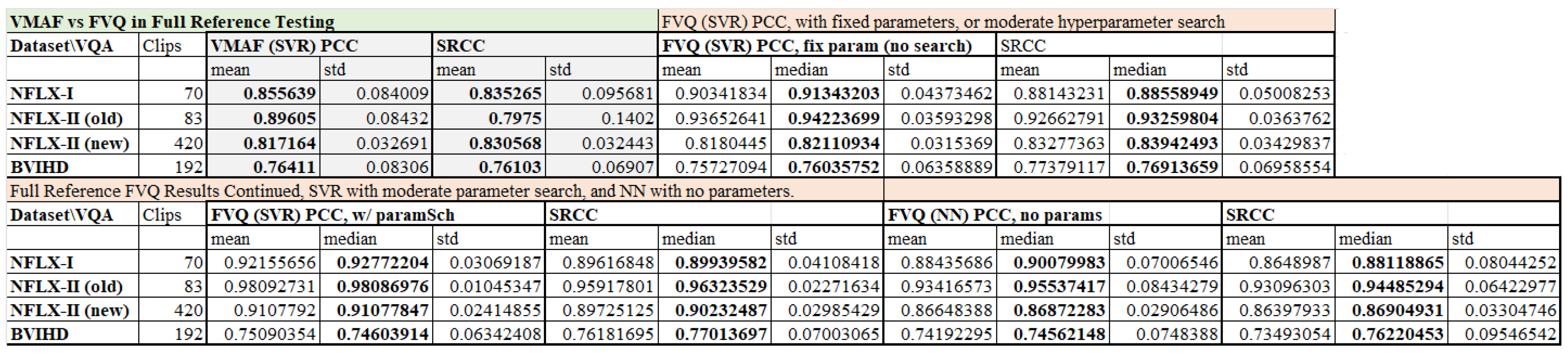
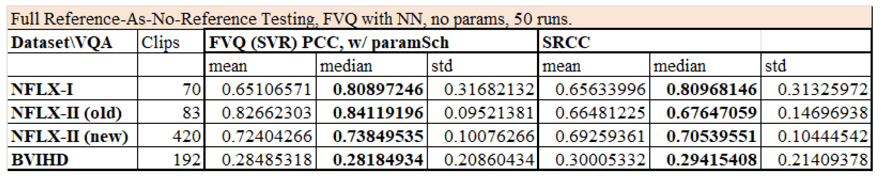
Perf.	0.705	0.819	0.788	0.741	0.931	0.928	0.927

provides some exemplary performance results of VMAF against various known VQAs, showing its excellent performance when well trained.

Table 2. Example performance of known VQAs in (a) the FR case by FastVDO, with no pretrained models; and in (b) the NR case, with UT-Google [10], using heavily trained models. While the FR case achieved useful levels of correlation with viewer ratings, the state of NR was more challenging. Recent advances have led to progress. Our FVQ achieved strong results in FR without pre-training; see Figure 2.

FV-Nflx2			UT-YTugc
FR-VQA	PCC	SRCC	NR-VQA	PCC	SRCC
PSNR	0.6982	0.6912	V-BLIINDS	0.559	0.5551
MS-SSIM	0.7304	0.7118	TLVQM	0.6693	0.659
SSIM	0.7334	0.7123	VIDEVAL	0.7787	0.7733
VMAF	0.8659	0.8432	RAPIQUE	0.7591	0.7684

provides some performance results in both FR and NR cases, again for benchmarking purposes.

$$\begin{array}{cc}\hfill & SAFD=\sum _{k=1}^K\left||F\left(k\right)-F(k-1)|\right|.(Actuallyuse\hfill \\ \hfill & \sum _{k=1}^{K-1}min\left(\right|\left|F\right(k)-F(k-1\left)\right||,|\left|F\right(k+1)-F(k\left)\right|\left|\right))\hfill \end{array}$$

(4)

Recently, this list of features was expanded to eleven, with two motion features (one taking the min above, the other not), DLM (called ADM) and four additional DLM features at the same scales (0–3) as the four scaled VIF features. To this list, FastVDO adds one or two more motion features, described below. Note that the Netflix motion features, computed only on the original video, contain no information about the loss of motion fidelity in the compressed or processed video. Nevertheless, as it does carry motion information, it performs well in predicting visual quality when fully trained, on test data such as the Netflix dataset [5]. Further enhancements of VMAF were reported in [21], which improved temporal information, but increased complexity. However, as we witnessed in our tests, where we trained VMAF from scratch, it performs well below the 90% level (see Figure 2), with the BVIHD dataset [22] proving to be especially challenging (76% in both PCC and SRCC). It proved challenging for our variants as well.

Relative to VMAF, we aimed to improve on both the quality of motion representation, as well as on the learning-based regressor engine. Specifically, for original video frames F(k), k = 0,…,K, and processed (distorted) video frames G(k), k = 0,…,K, since the temporal frame difference precisely corresponded to motion (all changes to pixels), we developed temporal motion-based metrics using the difference of frame differences (Equation (5)). Let us call this feature DM for differential motion. We retained the VIF and DLM features too. Like VMAF, we were able to use a range of features, from the base six (DM, DLM, VIF0-VIF3), up to a max of thirteen, where we added two variants of DM to the eleven current features of VMAF. We called our version of these features the FVMAF features. Importantly, we advanced the learning-based regressor engine to include feedforward neural networks (NNs), besides the SVR. One advantage of NN regression is that even without a computationally expensive hyperparameter search, it can provide excellent results. Our general framework is demonstrated in Figure 2.

$$\begin{array}{cc}\hfill & DM=\left|\right|\left(F\right(k)-F(k-1\left)\right)-\left(G\right(k)-G(k-1\left)\right)\left|\right|,\hfill \\ \hfill & theL1norm(butcanbeL2,Lp,Entropy,etc).\hfill \end{array}$$

(5)

We see that this is the simplest form of motion error analysis in the FR case, and there were analogs in the NR case. This can be generalized by analyzing motion flow in a local group of frames around at time t, say frames F(k), G(k), with k = t − L, t − L + 1, …, t, t + 1, …, t + L, and L > 0. Moreover, one can capture motion information either by fixed function optical flow analysis, or by using 3D convolutional neural networks, such as ResNet3D [23], as both C3DVQA and PVQ do. The trend is in fact to use learning-based methods for both feature extraction and regression, leading to an all learning-based VQA, in both FR and NR.

Figure 5. Example images from the following three databases under test: (left) BVI-HD [22]; (center) NFLX-II [5]; and (right) YouTube UGC [24]. The BVI-HD and NFLX-II databases have originals of high-quality, stable videos. The huge YouTube UGC dataset has mostly modest quality, user-generated videos, but with its wide variety, it even has 4K HDR clips.

Figure 5. Example images from the following three databases under test: (left) BVI-HD [22]; (center) NFLX-II [5]; and (right) YouTube UGC [24]. The BVI-HD and NFLX-II databases have originals of high-quality, stable videos. The huge YouTube UGC dataset has mostly modest quality, user-generated videos, but with its wide variety, it even has 4K HDR clips.

4. No Reference (NR) VQAs

Historically, FR VQAs have been mainly used as image quality assessments (IQAs), applied per frame and averaged. PSNR and SSIM are common examples. This can also be completed in the NR context, e.g., NIQE IQA [25]. The first completely blind NR VQA was released in 2016, namely the Video Intrinsic Integrity and Distortion Evaluation Oracle (VIIDEO) [7], based on NIQE IQA. This is an explicit, purely algorithmic approach without any prior training. It relies on a theorized statistical feature of natural images [26], captured as Natural Scene Statistics (NSS), and measured in the temporal domain. Analyzing frame differences, in local patches, they normalized the patch pixels by subtracting the mean, dividing by the standard deviation, modelling the resulting patch pixel data as a generalized Gaussian distribution, and estimating its shape parameters. Natural (undistorted) images have Gaussian statistics, while the distortions alter the shape parameter, which then leads to a distortion measure. An important fact is that this NR VQA already beats the common MSE, an FR VQA. Figure 5 provides example images from FR datasets BVIHD [22], NFLX-2 [5], and the NR dataset YouTube UGC [24]. A follow-on NR VQA called SLEEQ [8] was developed in 2018, which developed the NSS concept further. Meanwhile, [27] from 2018 repurposes image classifiers such as Inception to create a NR IQA, while [28] asks whether VQA is even a regression or a classification problem.

To summarizee the trends in this field, first note that as there was no original reference to compare to, they created a “self-referenced” comparator by blurring the compressed (or processed) video with a Gaussian blur, whose standard deviation then acted as a design parameter. The compressed and blurred compressed videos were then compared in patches, in both spatial and temporal domains, to create individual spatio-temporal distortion measures, which were then combined. As the recent paper [29] indicates, the performance of leading NR VQAs highlights significant challenges; see Table 2.

Given these limitations, a comprehensive analysis of the proposed methods was undertaken in 2020 in [9] for the NR case. In the analysis, the authors reviewed a vast array of NR algorithms, which they viewed as merely providing features to process. They began with no less than 763 features, then downselected to 60 features using the learning methods of support vector machines (SVM) and Random Forests. These 60 features were then aggregated using a highly optimized support vector regressor (SVR) with hyperparameters optimization to achieve performance, just under the 80% level in NR VQA [9]. While impressive, its complexity is high (though recently reduced in [30]), something both this paper and RAPIQUE [10] aimed to address. RAPIQUE uses a mixture of fixed-function and neural net based features, creating a huge 3884-dimensional feature vector, yet offered some speed gains over VIDEVAL due to the nested structure of features. Similarly, CNN-TLVQM [31] also used a mix of fixed-function and CNN-based features for the NR case, and reported strong results. Additionally, this trend is also in line with MDTVSFA [12] and PVQ [14]. We noted that both PVQ and MDTVSFA currently exceeded 80% performance on test sets, setting the current record. Meanwhile, a recent report from Moscow State University [32] even reported an achievement of over 90% correlation to human ratings, on par with the best FR algorithms, a result that remains to be confirmed by other labs.

5. FVQ: First Steps toward a Unified VQA

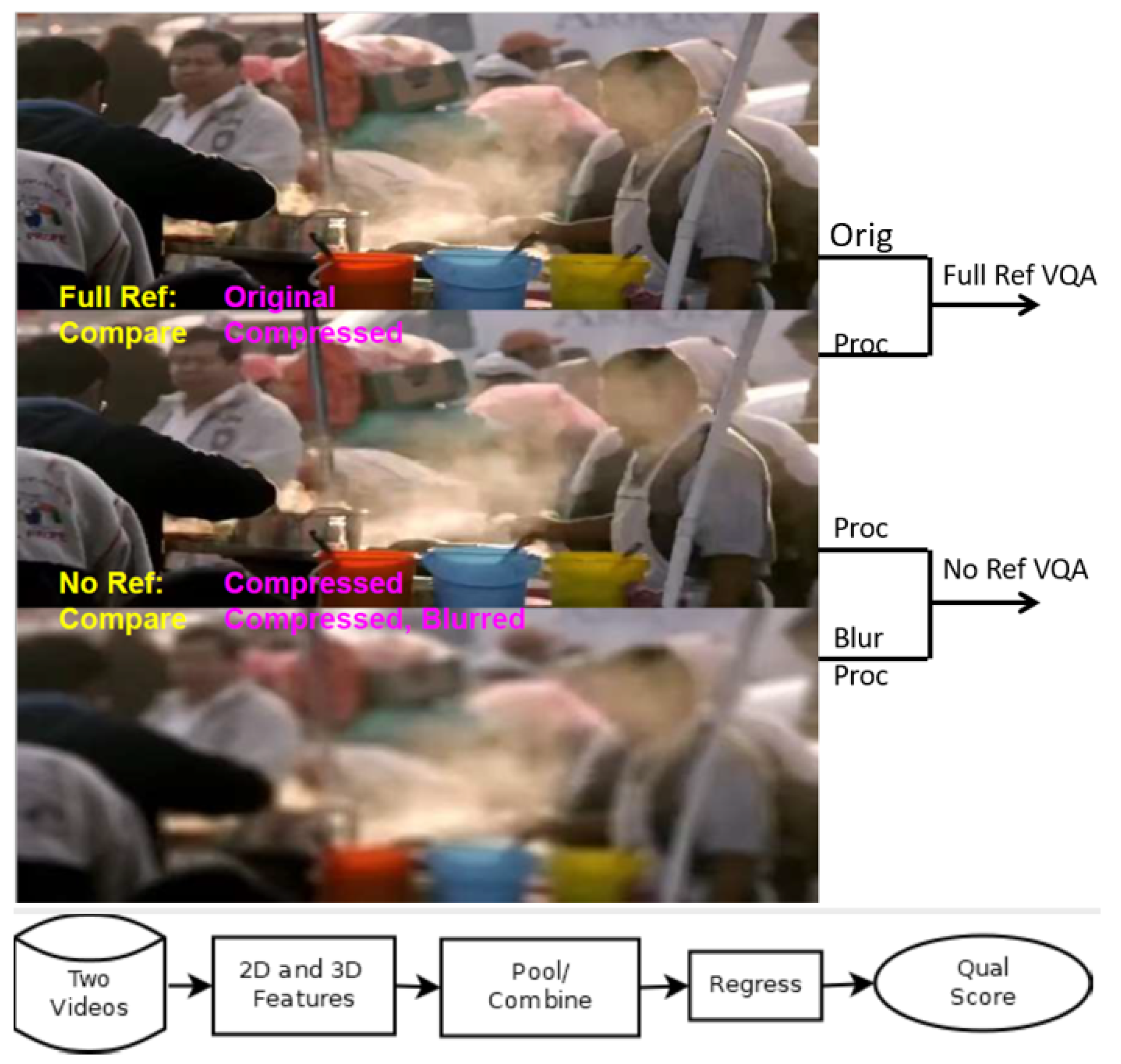
Combining insights from both the FR and NR cases, as exemplified by VMAF and SLEEQ, we arrived at a partial synthesis; see Figure 1. In FR, we compared a processed video to the original; in NR, we compared it to a blurred processed video. In both cases, we input two videos, extracted spatio-temporal (that is, 2D and 3D) features, passed them to a regressor engine, and obtained a quality score. The feature extractor and the regressor can both use learning-based methods such as SVRs and neural nets. Purely for complexity reasons, we currently prefer fixed-function feature extractors, but note that CNN-based features are quite popular [10,11,12,14], and also used them. 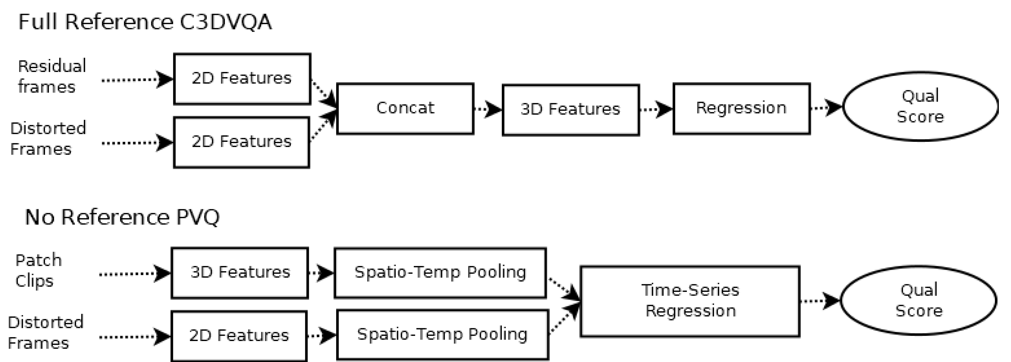Note that not only VMAF and FVMAF algorithms fit into the general FVQ framework of Figure 1, but very broadly, so do C3DVQA and PVQ. One small difference is that C3DVQA computes 2D and 3D features serially, while PVQ does so in parallel; see Figure 6. However, at least at a high level, there remain some similarities. Moreover, we demonstrated that if the FR case was treated as an NR case, our approach still yielded quite usable predictions, with roughly 75% prediction accuracy, partially justifying our attempted synthesis. While the similarities between FR and NR currently do not persist at finer levels of detail, this viewpoint can at least suggest next steps in research. Meanwhile, we remark that MDTVSFA computes only 2D features, but the 3D analysis was performed at the quality score level, which is unusual and differs from our framework.

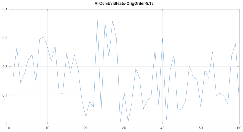
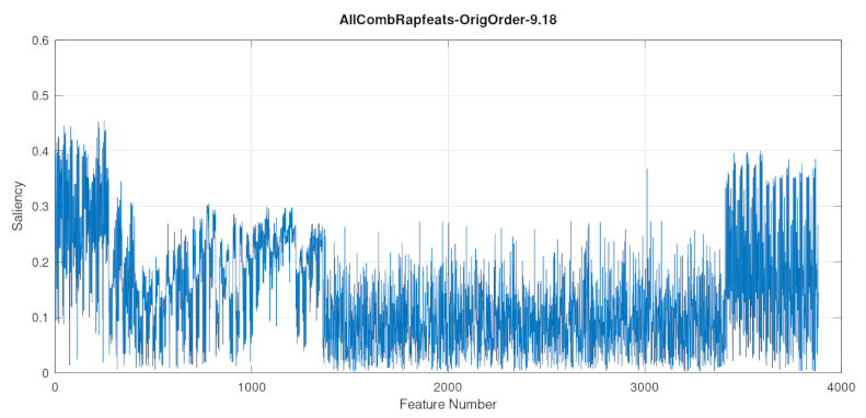
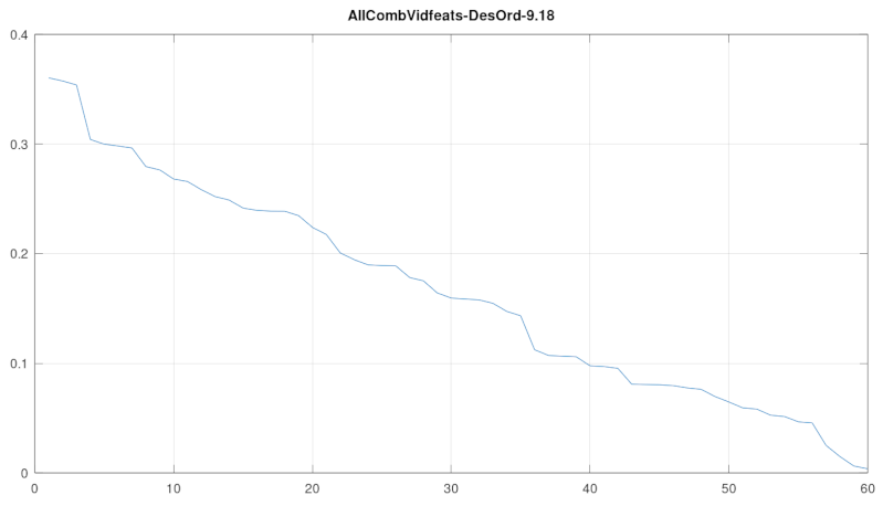
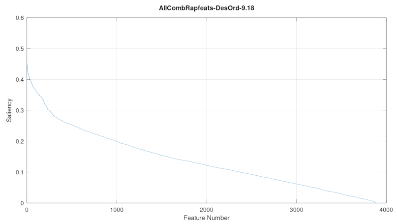
Given the variety of approaches to extracting features, features can also be mixed and matched at will to optimize performance; and if desired, we can always add the output score of any NR algorithm as an additional feature in any NR or FR VQA. To that end, we developed a simple Feature Saliency measure, which can help pick the most useful features to employ.

5.1. Feature Saliency and Selection

For high-quality FR databases, our FVMAF features were nearly the same as for VMAF (but with a substituted motion feature, DM). We can also apply these same type of features in NR testing. However, for challenging user generated content (UGC), our FVMAF features proved highly inadequate. So, we utilized the powerful features from [9,10]; see Figure 4, Figure 7 and Figure 8, and

Table 3. Row 1: Features from (a) VIDEVAL and (b) RAPIQUE, for the AllCombined NR dataset, in original order. Row 2: Same features in descending Saliency order. Row 3: Prediction performance under a FastVDO parameter-free neural network regressor, over 50 runs, using the first N Saliency-ordered features. Row 4: Saliency ordering of mixed VIDEVAL/RAPIQUE features, and correlation coefficients PCC and SRCC using the Saliency-ordered features. Our best results are with all 60 VIDEVAL and the top 120 RAPIQUE features, reported in the last row of Figure 4. While our approach did not achieve state-of-the-art performance, we did clarify that just a few of the most salient features from each algorithm provided most of the predictive performance.

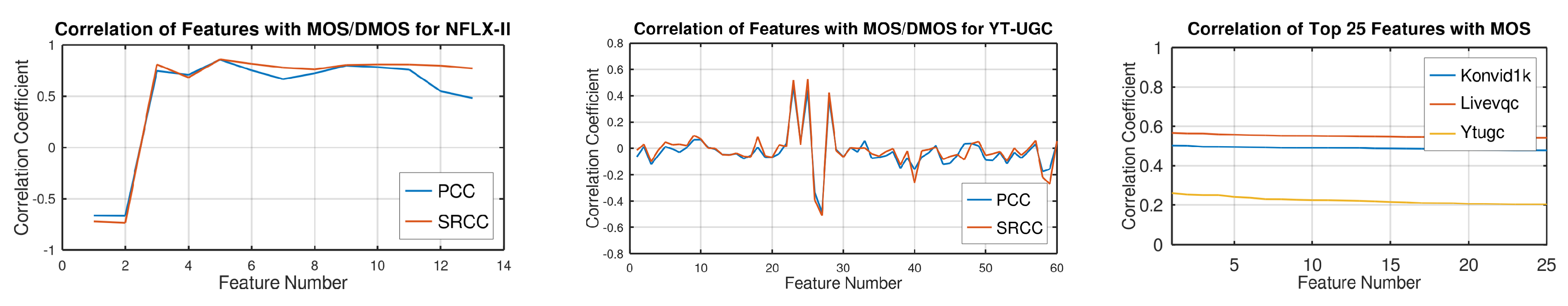
Nr.	a	b
1
2
3
4

. We selected a subset of features using a simple Feature Saliency measure described here. We ordered the features according to a novel combined correlation coefficient measure S(f) (Equation (6)), and typically selected a subset of the top ranked features. For example, out of the 3884 RAPIQUE features, we selected only 200; see Table 3. Here = 0.5 by default, but this can be modified to favor PCC or SRCC.

$$\begin{array}{cc}\hfill & S\left(f\right)=\alpha \ast \left|PCC\right|+(1-\alpha )\ast \left|SRCC\right|;\alpha =0.5bydefault.\hfill \end{array}$$

(6)

5.2. Regression

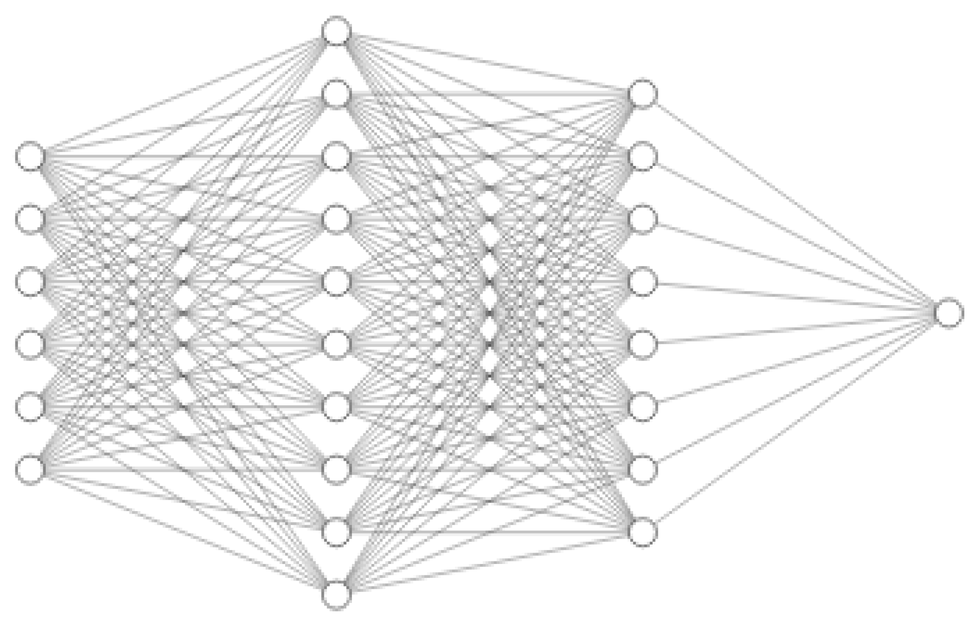
For regression, we used both SVRs and simple feedforward fully-connected NNs. For the SVR, we conducted a limited hyperparameter search for the parameters known as C, gamma, epsilon. For the neural net, we used a very simple fully connected feedforward network; as an example, with six features, we used a 6-80-64-1 network, with Relu activation, RMSProp optimizer, and Tensorflow 2.4.1, to aggregate the features (we occasionally used sigmoid activation in the last layer); see Figure 9. Post feature extraction, the example total train/test simulation time for 1k sims of SVR was only 10 s to run (no-GPU) in FR, while 50 sims of NN took 127 s on a laptop (i7-10750, 16 GB RAM, RTX 2070 GPU). In NR, our SVR inference time with our reduced parameter search required only 4 s; while the post parameter search only lasted 0.01 s.

For direct comparisons in trainability, we used the same train and test regimen as our comparators, and trained from scratch. In the FR case, when comparing with VMAF, we used essentially the same features and SVR settings as VMAF; however, we changed the motion feature, and improved some hyperparameters. Our fixed SVR parameters were (C, eps, gam) = (1000, 1, 0.1), while for moderate search, we searched (C, eps, gam) in the ranges ([10, 100, 900, 1000], [0.01, 0.05, 0.1, 0.5, 1], [0.0001, 0.001, 0.01, 0.1, 1]). In the NR case, we used the 60 VIDEVAL features, the same SVR framework and hyperparameter set, or else a no parameter search neural network. We also tested around 100 of the RAPIQUE features with subsets (out of 3884). Our results in the FR case indicated that both our SVR and NN methods outperformed VMAF (Figure 2). Additionally, even when ignoring the reference on FR data, we obtained useful results with the same type of features and regressors, partially validating our unified approach (Figure 3). 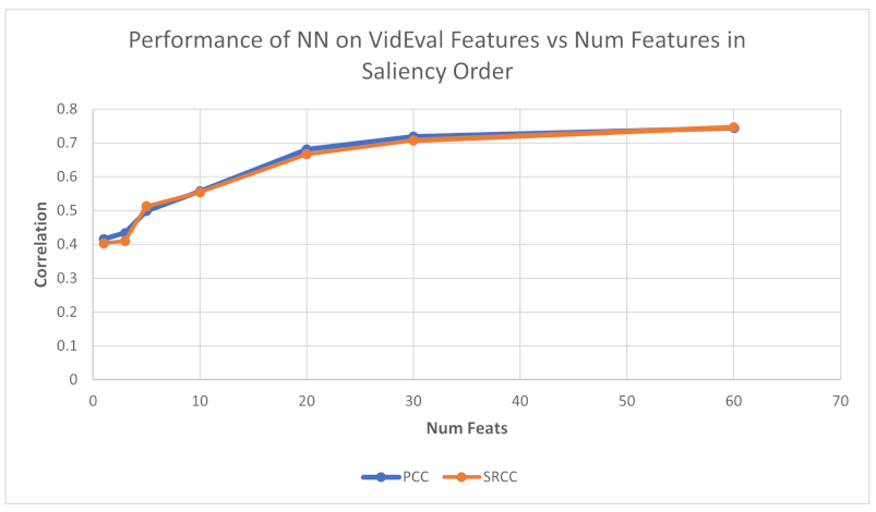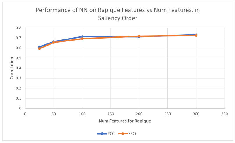In the NR case with challenging UGC datasets, even when compared to the fully trained VIDEVAL or RAPIQUE algorithms, our correlation scores were competitive, while greatly reducing the hyperparameter search complexity during training (Figure 4 and Table 3). In fact, with both SVR and short NN, since today’s TPUs can process FFNNs in real-time on at least a 1080p30 resolution, the main complexity in execution now lies in the feature extraction phase. Thus, limiting the expensive feature extraction part is critical to live usability. For FR, we mainly used just six features; for NR, we tested with 10-400 features, drawn from VIDEVAL, RAPIQUE, or both. To date, we have not tested features from MDTVSFA or PVQ in our framework.

5.3. Results and Discussion

Figure 2 and Figure 3 present our main results for the FR case. In FR, we used features identical to the VMAF features but with an improved motion feature, and use improved regression using a parametric SVR, or a neural network. We obtained results across several datasets that exceed VMAF in both PCC and SRCC by roughly 5%, and up to 15%, which is a substantial gain. Achieving roughly 90% across datasets for both PCC and SRCC, with no prior training, this technology appeared to mature. (However, one dataset, BVIHD, proved to be highly challenging for both VMAF and our methods.) Moreover, gains were achieved with no increase in training/testing complexity with either the SVR with fixed parameters, or the NN with no parameter search. With moderate search using the SVR, we were able to obtain some further gains; see Figure 2. Finally, even if we ignored the reference videos and viewed these datasets as NR, we still obtained useful results, again using a no-parameter NN regressor. It is this finding that partially validated our attempted synthesis of FR and NR in one framework; see Figure 3. However, this is still simulated NR in the high-quality domain of professional video.

In the true NR case of UGC data, our FVMAF features were inadequate, and we must leverage the impressive work in VIDEVAL and RAPIQUE in developing powerful features. Faced with thousands of features, we worked to reduce the feature sets, while still obtaining results close to these SoTa algorithms. In particular, we elucidated the contribution of individual features using a novel saliency measure. In this paper, we mainly focused on compression and scaling loss, leaving aside generic transmission errors for now as they are less relevant with HTTP streaming. See Figure 4 and Table 3.

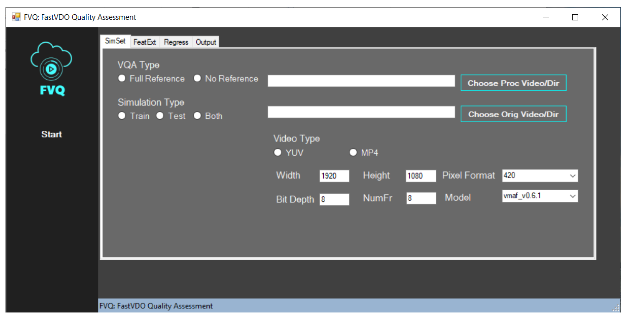
To assist in this research, we built a GUI-based application called FVQ, capable of executing both FR methods as VMAF and FVMAF, as well as NR methods such as RAPIQUE (which we have converted to python); Figure 8 provides a screenshot.

5.4. Focus on the No Reference Case

Good progress was made on the FR case, but much work remains for the growing NR case due to its challenges. Computationally, we noted that the FR VMAF features are few, fixed-function, integerized, multi-threaded, and fast; the VIDEVAL features are not, nor are the RAPIQUE features, which while many, are somewhat faster. However, both algorithms are currently only at the research level in Matlab (as is CNN-TLVQM). However, there has recently been a significant increase in the speed of VIDEVAL (VIDEVAL_light [30]) by downsampling feature extraction in space and time, with marginal loss. Much work is still needed in the NR case to achieve both the performance and execution speeds needed in live applications, but we will continue to make useful progress on that front, similar in spirit to RAPIQUE [10].

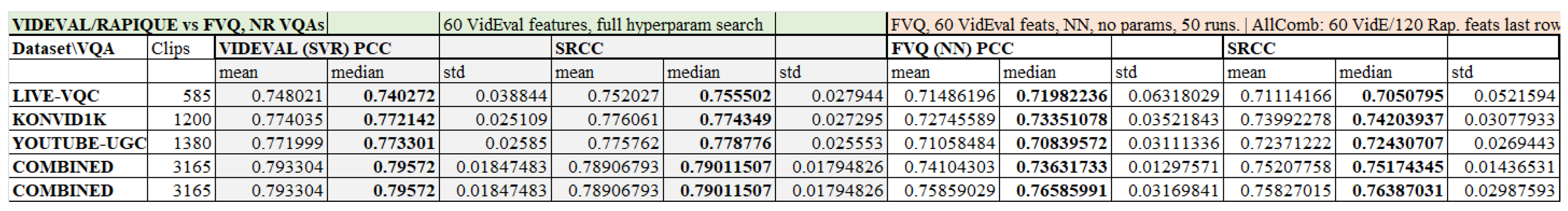
Meanwhile, we focused on the potential performance that can be achieved using the powerful features from VIDEVAL and RAPIQUE, but also our novel feature selection method prior to regression, if we choose to eliminate hyperparameter search during training. We see from Table 3 that for the AllCombined NR dataset with 3165 videos, just a few of the most salient features provided most of the predictive performance, via SVR or NN. Two advantages of the NN method are that (a) it is fast on a modern GPU, and (b) it does not require hyperparameter search during training, significantly enhancing the potential for live application. 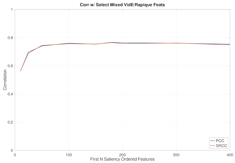We see from Figure 4 and Table 3 that, either using the 60 VIDEVAL features, or 100–200 mixed VIDEVAL and RAPIQUE features, we can reach within 3% of these algorithms on the AllCombined dataset, using a fixed architecture neural network, without any parameter search or parametric curve-fitted prediction. Our best NR result for the AllCombined dataset was obtained using all 60 VIDEVAL features, and 120 top RAPIQUE features (total of 180), obtaining PCC/SRCC of 0.766/0.764; see Figure 7. Moreover, the 50 cycles of training/testing in our neural network ran at least 20X faster than the SVR in a Google Colab tensorflow simulation environment. Additionally, our saliency analysis helped to elucidate which features were the most informative. To achieve new state-of-the-art performance in NR going forward, our plan is to incorporate additional powerful features (such as from [31]), use more extensive parametric search and use curve-fitting for SVR prediction (as in VIDEVAL and RAPIQUE), or use the power of NN regression more fully.

6. Conclusions

We investigated an approach to assessing video quality in both FR and NR cases using a generic framework, consisting of taking two input videos, i.e., original and processed or processed and blurred-processed, evaluating a variety of (fixed or learned) features on these videos, and regressing these using an SVR or a feedforward NN to obtain a score. In the FR case, taking inspiration from the excellent and well-established VMAF algorithm, we worked to create enhanced variations, using modifications of the feature set as well as the regressor, with improvements in the motion feature as well as a parametric SVR or an NN regressor. In the NR case, we developed on algorithms such as SLEEQ as well as VIDEVAL. While not achieving SoTa, we reduced the training complexity by eliminating hyperparameter search as well as reducing the number of features, yet achieved performance of close to VIDEVAL and RAPIQUE on the AllCombined dataset, and not far from that of the latest SoTa algorithms MDTVSFA and PVQ. In Figure 2, we suggested a path to at least partially unifying the FR and NR cases. While at a high level the example FR and NR algorithms in Figure 6 remained consistent with our general picture, they differed in detail, so that actual unification remains a problem. Much more research remains to be conducted to achieve either true unification, or a new state-of-the-art algorithm in performance for NR applications.