A Novel Approach Based on IoT and Log-Normal Distribution for Supplier Lead Time Optimization in Smart Engineer-to-Order Supply Chains

Abstract

Background: In Engineer-to-Order (EtO) supply chains, managing supplier lead times is particularly challenging due to high customization and intensive customer involvement. This study addresses the critical need for more accurate and dynamic lead time prediction to enhance supply chain resilience and efficiency in EtO environments. Methods: We propose a novel approach that integrates Internet of Things (IoT) technologies with statistical modeling using the log-normal distribution to model and optimize supplier lead times, especially for customized raw materials. The model incorporates real-time data from IoT-enabled suppliers and considers long-term contractual relationships to reduce variability. Monte Carlo simulation is employed to validate the model’s predictive capabilities. Results: The results demonstrate significant improvements in predicting supplier performance and reducing uncertainty. Simulation outputs reveal reductions in lead times and enhanced reliability. Statistical metrics such as the Mean Absolute Error (MAE) and Root Mean Square Error (RMSE) confirm the robustness and accuracy of the predictions. Conclusions: The proposed methodology supports better decision-making in supplier selection and procurement planning by enabling effective risk management. It contributes to improved performance and greater resilience in Engineer-to-Order supply chains.

1. Introduction

Engineer-to-Order (EtO) production environments are defined by their high level of customization, where products are engineered and manufactured only after a specific customer order is received. This configuration allows manufacturers to respond to unique specifications but introduces significant operational challenges, notably in managing supplier lead times. In EtO settings, long and variable lead times—driven by design complexity, supplier constraints, and dynamic coordination—can severely affect production flow, cost control, and customer satisfaction. While the variability in lead time is well acknowledged in supply chain literature, it remains one of the most difficult parameters to model and predict accurately in the context of customized manufacturing.

Over the past decades, researchers have proposed various tools and frameworks to improve planning and performance in EtO systems, including methods for bid evaluation, capacity management, project scheduling, and production control. Yet, most of these models fall short when addressing the core challenge of lead time uncertainty. A major limitation is the continued reliance on assumptions of normality in lead time behavior, which tend to simplify analysis but fail to reflect the asymmetric, long-tailed, and non-negative distributions typically observed in real-world EtO supply chains. Consequently, traditional models often underestimate the risk of extreme delays, leading to understocking, missed deadlines, and unreliable planning.

This paper presents a new modeling framework for supplier lead time prediction in EtO environments, which combines two complementary perspectives: a statistical model based on the log-normal distribution, and a real-time adjustment layer driven by Internet of Things (IoT) data. The log-normal distribution is particularly well suited for this purpose due to its ability to represent positively skewed and multiplicative phenomena, while IoT technologies provide the capability to dynamically update forecasts in response to live operational signals from suppliers, production systems, or transport processes.

The existing literature offers important insights into the nature of lead time variability. Pioneering works by Tadikamalla [1], Das [2], and Aggarwal [3] highlighted the benefits of using log-normal assumptions for lead time demand modeling, particularly in settings marked by demand uncertainty and nonlinearity. Further evaluations by Strijbosch and Moors [4] and Tyworth [5] explored alternative distributions such as truncated normal and gamma, affirming that standard models are often inadequate under conditions of asymmetry and high variability. More recent contributions have shifted attention toward smart forecasting frameworks, as seen in De Simone et al. [6], who emphasized the need to incorporate workforce dynamics and operational feedback in lead time estimation, particularly for small and medium-sized enterprises (SMEs).

Recent studies further reinforce the role of IoT in enabling predictive adaptability and real-time responsiveness across the supply chain. For instance, Alzahrani and Asghar [7] proposed an IoT-based system to enhance logistics risk prediction. Sallam et al. [8] emphasized best practices and challenges in IoT adoption, stressing its role in improving visibility and responsiveness. Zrelli and Rejeb [9] also underscored the increasing relevance of IoT in supply chain forecasting and performance optimization.

Building on these foundations, this research proposes a hybrid predictive framework that captures the stochastic nature of supplier lead time through log-normal modeling and enhances its accuracy by integrating IoT-based signals. The approach is tested through Monte Carlo simulation under varying degrees of lead time variability—low, medium, high, and very high—and evaluated against traditional normal-distribution-based models using error metrics such as the Mean Absolute Error (MAE) and Root Mean Square Error (RMSE).

In addition to proposing a robust mathematical model, this research highlights the strategic importance of long-term contracts with suppliers of customized raw materials. Such agreements can reduce variability and enhance supply chain resilience, making predictive models more reliable.

The results show that the proposed model significantly improves forecasting performance, especially under high- and very-high-variability scenarios. It offers better alignment with real operational behavior and supports more informed decision-making in EtO planning and procurement processes. Furthermore, the model’s architecture allows for extension into real-time applications such as digital twins, decision support systems, and intelligent procurement platforms.

The remainder of this article is structured as follows: Section 2 provides a comprehensive review of the existing literature; Section 3 outlines the problem statement and research motivations; Section 4 introduces the proposed framework and describes the methodology; Section 5 presents and analyzes the simulation results; Section 6 discusses the broader implications of the study, addresses its limitations, and proposes directions for future research; and finally, Section 7 concludes the paper by summarizing the key contributions and highlighting practical and theoretical takeaways.

2. Literature Review

Lead time variability is a well-known issue in supply chain management, especially in EtO industries where customization leads to longer and more unpredictable lead times.

In recent years, several studies have addressed various issues in the EtO industry, proposing different approaches and solutions to improve performance and efficiency. These studies have focused on diverse areas such as bid solution uncertainty, capacity planning, lead time reduction, workflow visibility, and scheduling, among others. However, each of these approaches comes with its own contributions and limitations [10].

For example, the challenge of bid solution uncertainty has been tackled using multi-criteria approaches, such as a multi-criteria bid solution model that provides accurate and timely replies to bid requests, but it is limited by the scope of a single case study with restricted data [11]. Similarly, another study introduces an interactive bid solution evaluation, allowing for optimal bidder decision-making, but it becomes time-consuming due to the many criteria involved [12]. In the realm of capacity planning, tactical capacity planning with an optimization model has improved decision-making for planning but suffers from a lack of broad case studies [13].

One prominent issue in the EtO industry is long lead times. To address this, Simio software simulation has been used to reduce costs and shorten lead times, but frequent design changes can significantly disrupt the replanning process [14]. Similarly, Quick Response Manufacturing (QRM) has been implemented to enhance customer responsiveness through hybrid architectures, yet it requires a more organized technological infrastructure [15].

Another area of concern is the frequent design changes in the EtO process. A Lean Project Management approach was applied to combine lean efficiency with flexibility, addressing these frequent changes. However, real-world applications would benefit from more dynamic and agile approaches to face these challenges more effectively [16].

In terms of production scheduling, several solutions have been proposed, such as the use of Kanban panels to manage PERT/CPM tasks, but these systems require further practical applications to validate their utility [17]. Another contribution is the hyper-heuristic improved genetic algorithm for scheduling, which improves algorithm efficiency, though it faces limitations when dealing with large-sized problems [18].

In inventory and supply chain management, particularly in contexts characterized by high variability and asymmetric distributions such as the Engineer-to-Order (EtO) environment, the log-normal distribution has been recognized as a robust modeling tool. The log-normal distribution is strictly positive and skewed to the right, making it particularly appropriate for modeling variables such as supplier lead time, where delays tend to be more extreme than early arrivals. Tadikamalla [1] was among the first to demonstrate the effectiveness of using the log-normal distribution to approximate the demand during lead time in stock control problems, emphasizing its simplicity compared to the gamma distribution. Later, Das [2] developed analytical expressions based on the log-normal assumption for expected demand over lead time in reorder point models. Aggarwal [3] extended the application to finished goods inventory systems, and further comparisons by Tadikamalla [19] with five other distributions confirmed that the log-normal, gamma, and Weibull distributions perform best when the coefficient of variation is high. Importantly, the log-normal distribution was found to balance both computational simplicity and modeling accuracy. More recently, Strijbosch and Moors [4] highlighted the limitations of the normal distribution—especially its allowance of negative values—and proposed modified and truncated versions to address these issues. Nonetheless, the log-normal distribution remains a preferred choice when modeling variables that are both multiplicative in nature and strictly positive, such as supplier lead times in EtO environments. Al-Harkan and Hariga [20] also employed the log-normal distribution to model continuous review inventory systems, and they found that the log-normal distribution is especially useful when both variables are uncertain, as it enables better representation of volatility in complex production environments reinforcing its validity in stochastic supply settings. Given that lead times in EtO are influenced by various multiplicative factors—such as component complexity, customization level, and supplier responsiveness—the log-normal distribution emerges as a theoretically sound and empirically supported modeling choice.

The integration of IoT-enabled data streams into supply chain forecasting models has become increasingly essential, particularly in dynamic and high-variability environments. Recent studies highlight the value of IoT in enhancing forecasting precision through real-time visibility, condition monitoring, and disruption detection. For instance, Alzahrani and Asghar [7] developed an intelligent risk prediction system that utilizes IoT data in logistics, improving proactive decision-making and responsiveness across the supply chain. Zrelli and Rejeb [9], through a bibliometric analysis, confirmed the growing academic and industrial focus on IoT applications in logistics, particularly for predictive analytics and real-time coordination. Additionally, Sallam et al. [8] outlined key challenges and best practices in IoT integration, emphasizing the importance of interoperability, security, and real-time data analytics to enhance operational efficiency. In parallel, digital twin technologies have emerged as a powerful complement to IoT-based forecasting systems. Abideen et al. [21] proposed a digital twin model enhanced with reinforcement learning for improved decision-making in logistics and supply chains. Similarly, Kritzinger et al. [22] classified digital twin applications in manufacturing, highlighting their potential for simulating complex systems and predicting disruptions. Collectively, these studies reinforce the consensus that real-time IoT data and digital representations—particularly digital twins—significantly improve forecast accuracy, resilience, and responsiveness in complex supply networks.

Overall, while these approaches have contributed significantly to improving different aspects of the EtO process, including lead time prediction, bid solution optimization, and workflow visibility, the literature highlights that many of these solutions are constrained by limited case studies, insufficient data, and technological integration issues. This presents the need to focus on broader applications and more integrated systems.

3. Problem Statement: Current Practices and Gaps in Lead Time Prediction for EtO Supply Chains

A careful analysis of two recent and comprehensive systematic literature reviews has highlighted significant shortcomings in existing research. First, Burggräf et al. [23] emphasized that the majority of lead time prediction models in EtO settings focus primarily on order- and system-level data, with limited integration of material-level data, especially for customized components. They also noted that these models are generally static, offering little capability for real-time responsiveness or the incorporation of data from Internet of Things (IoT) sources. Second, Fortes et al. [10] reviewed a broad range of EtO-related solutions—including bidding strategies, RFID implementations, scheduling, and capacity planning—and found that most of these approaches suffer from limited technological integration, insufficient adaptability, and a lack of scalable, dynamic modeling frameworks suitable for volatile supply chain environments.

Based on insights from these reviews and our own synthesis of the recent literature, four critical research gaps were identified: (1) the absence of predictive models specifically focused on supplier lead times for customized raw materials in EtO supply chains; (2) the underutilization of log-normal probabilistic modeling, despite its well-documented suitability for representing positively skewed, non-negative lead time distributions; (3) the lack of predictive models that dynamically adjust lead time forecasts using real-time data inputs, such as IoT-enabled signals from suppliers or logistics networks; (4) a lack of simulation-based validation of prediction models across different variability scenarios, which is essential for testing robustness under uncertainty.

This study addresses these gaps by proposing a log-normal-based predictive modeling framework enhanced with real-time IoT-based dynamic adjustments and validated through Monte Carlo simulations. By doing so, it contributes to the development of scalable, resilient forecasting tools tailored to the specific complexities of EtO environments.

4. Methodology

This study adopts a quantitative, simulation-based methodology that combines mathematical modeling, IoT-based adjustment, probability theory, and simulation techniques to predict supplier lead times in an EtO supply chain, with a specific focus on customized raw materials. Due to the unavailability of real historical lead time data, a Monte Carlo simulation was conducted to generate synthetic supplier lead time datasets under four variability scenarios: low variability (σ = 0.2), medium variability (σ = 0.5), high variability (σ = 0.9), and very high variability (σ = 1.2). These simulated data points were then modeled using the log-normal distribution, selected for its ability to accurately represent the natural skewness and variability observed in real-world supplier lead times.

Once the simulated lead times were generated, prediction models based on the log-normal distribution were developed, and real-time adjustment factors—representing disruptions such as production delays or transportation issues—were simulated to dynamically modify the predicted lead times, simulating the potential influence of IoT-based updates.

A series of Monte Carlo simulations were performed for each scenario to produce a broad range of possible outcomes, enabling the assessment of prediction accuracy and uncertainty. The performance of the log-normal-based predictions was compared against traditional normal distribution-based predictions using statistical accuracy metrics such as MAE and RMSE.

In the context of EtO supply chains, especially when dealing with customized raw materials, establishing long-term contracts with strategic suppliers is a fundamental prerequisite for ensuring data reliability and operational coordination. This enduring relationship facilitates the seamless integration of IoT devices at the supplier’s premises, enabling real-time data acquisition on production status, dispatch times, and potential disruptions. By fostering this collaborative environment, companies can obtain consistent, high-quality data streams, which are essential for calibrating and dynamically adjusting predictive models. The methodology proposed in this study, therefore, emphasizes the importance of securing long-term supplier agreements as a critical foundation for deploying IoT-based predictive analytics and enhancing the accuracy and responsiveness of lead time forecasting.

In parallel, we propose an alternative operational framework intended for real-world industrial application. In this applied framework, companies would utilize actual historical supplier lead time data, complemented by real-time IoT sensor data, to continuously update and refine their supplier lead time predictions. Monte Carlo simulations could then be employed for risk analysis and scenario testing purposes, providing decision-makers with a realistic, data-driven tool to improve responsiveness and resilience in the EtO supply chain environment. As part of the proposed architecture for integrating IoT into dynamic supplier lead time prediction, several sensor technologies and data flows are envisaged, in alignment with current industry practices and recent research in smart supply chains. Machine status and environmental sensors—including vibration, temperature, load, and runtime sensors—installed on critical supplier equipment can detect production slowdowns, maintenance needs, or quality issues. Logistics tracking devices, such as GPS modules, RFID tags, and vehicle telematics systems, provide real-time updates on shipment movements, delays, and estimated arrival times—key for lead time prediction in Engineer-to-Order (EtO) environments, where component availability is tightly linked to production schedules. Warehouse and dispatch monitoring tools, including barcode scanners, automated storage systems, and weight sensors, help track inventory flow and delivery readiness for customized raw materials. Additionally, edge IoT devices and communication gateways perform local preprocessing of sensor data and transmit only critical anomalies or status changes to centralized analytics platforms. This aligns with edge computing architectures that aim to improve responsiveness while minimizing network load. These sensor types collectively generate real-time data flows that feed into the dynamic adjustment factor δ(t) in our predictive model, enabling continuous lead time updates in response to actual operational fluctuations.

4.1. Architecture Overview of the Proposed Approach

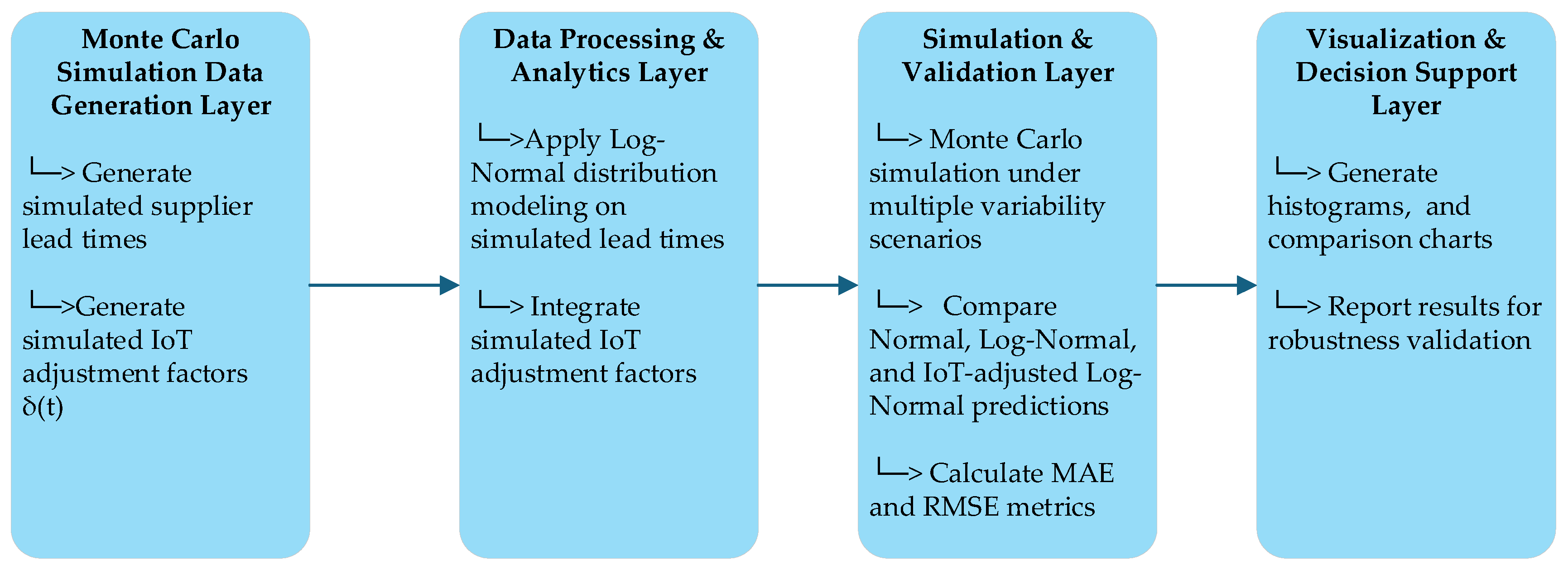
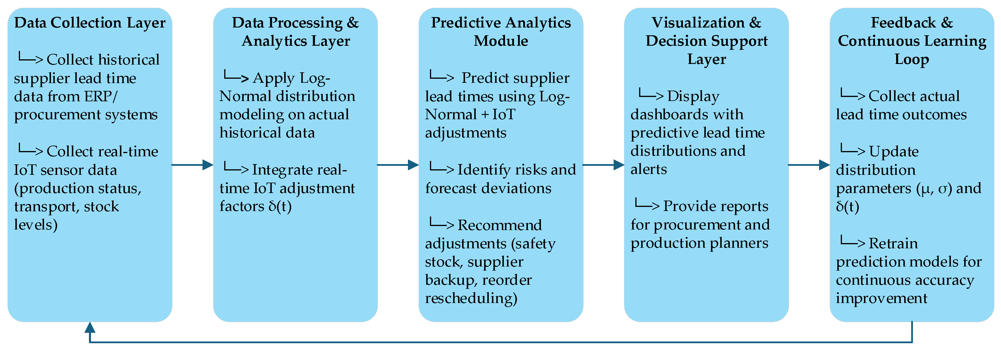
To provide a comprehensive view of the proposed methodology and its potential real-world application, two architectural frameworks are presented. The first architecture (Figure 1) illustrates the simulation-driven approach applied in this study, where synthetic data generation, probabilistic modeling, and Monte Carlo simulation were used to validate the robustness of the proposed predictive method. The second architecture (Figure 2) represents a practical operational framework that companies and EtO industries could adopt when actual historical lead time data and IoT-enabled infrastructure are available. This operational framework integrates real historical data, real-time IoT feedback, predictive analytics, and continuous learning mechanisms to support intelligent, data-driven supplier lead time predictions in smart EtO supply chains.

4.2. Proposed Mathematical Model

This section presents the mathematical formulation of the lead time prediction model, the calculation of key statistical parameters, and the integration of IoT-based adjustments.

4.2.1. Log-Normal Distribution for Supplier Lead Time

The lead time Ts, for a customized raw material from a supplier, is modeled as a random variable following a log-normal distribution. The probability density function (PDF) of a log-normal distribution is given by the following:

$$f\left(Ts\right)={\displaystyle \frac{1}{Ts \sigma \sqrt{2\pi }}}\exp (-{\displaystyle \frac{(\ln Ts-\mu {)}^2}{2{\sigma }^2}})$$

(1)

where Ts represents the supplier lead time, μ represents the mean of the natural logarithm of the lead time, calculated by

$$\mu ={\displaystyle \frac{1}{n}}\sum _{i=1}^n\mathrm{l}\mathrm{n}\left(T_{si}\right)$$

(2)

n represents the number of simulated (or observed) supplier lead times (i.e., the sample size),$T_{si}$ represents the i- th simulated (or observed) supplier lead time, and σ represents the standard deviation of the natural logarithm of the lead time, calculated by the following:

$$\sigma =\sqrt{{\displaystyle \frac{1}{n-1}}\sum _{i=1}^n{(\ln T_{si}-\mu )}^2}$$

(3)

In the context of EtO, this model allows us to capture the variability and skewness in lead times. For example, most deliveries may occur within a short time frame, but there are non-negligible probabilities for longer delay.

4.2.2. Expected Lead Time

The expected lead time E [Ts] for a log-normal distribution is given by the following:

$$E\left[Ts\right]=exp(\mu +{\displaystyle \frac{{\sigma }^2}{2}})$$

(4)

This formula provides an estimation of the average lead time, adjusted for both the mean and variability of the supplier’s performance. It allows companies to plan their production schedules more effectively by considering the realistic expected lead times rather than just the average.

4.2.3. Variance and Risk in Lead Time

The variance Var (Ts) of the supplier lead time is calculated as follows:

$$Var\left(Ts\right)=(\mathrm{e}\mathrm{x}\mathrm{p}\left( {\sigma }^2\right)-1) \mathrm{e}\mathrm{x}\mathrm{p}(2\mu +{\sigma }^2)$$

(5)

This gives insight into the risk or uncertainty in the supplier’s performance. Higher variance indicates greater unpredictability, which needs to be factored into safety stock levels and delivery buffers.

4.2.4. Integration of IoT-Based Dynamic Adjustment Factor δ(t)

To enhance the accuracy and adaptability of supplier lead time predictions, we introduce a dynamic adjustment factor, δ(t), derived from real-time IoT sensor data. While the baseline lead time Ts is modeled using a log-normal distribution to capture natural variability and skewness, δ(t) represents a time-dependent percentage deviation that modifies this base prediction to reflect real-world operational fluctuations. Specifically, δ(t) is modeled as a bounded random variable ranging typically between -0.05 and +0.15, corresponding to a 5% reduction up to a 15% increase in lead time. Negative values simulate minor efficiency gains (e.g., early completions), whereas positive values represent delays caused by disruptions such as machine breakdowns, transportation bottlenecks, or supplier delays common in Engineer-to-Order (EtO) environments.

Under stable conditions without detected disruptions, δ(t) defaults to zero, preserving the baseline log-normal prediction. For simulation purposes, δ(t) is generated from a truncated normal distribution centered at zero with scenario-dependent variance, allowing it to realistically capture stochastic fluctuations informed by synthetic or real IoT inputs. In operational settings, δ(t) is updated dynamically in near real-time by aggregating data from diverse IoT sources, including machine health sensors (vibration, temperature), logistics trackers (GPS, RFID), and inventory monitors (barcode scans, dispatch readiness). This dynamic adjustment framework enables continuous refinement of lead time predictions as supply chain conditions evolve, supporting more responsive and informed decision-making in EtO supply chains.

The IoT-adjusted lead time is thus computed as follows:

$$T{s}_{IoT}=Ts (1+\delta (t\left)\right)$$

(6)

where the following obtains:

▪

Ts represents the log-normal predicted lead time obtained from the log-normal model;

▪

δ (t) is a dynamic adjustment factor derived from real-time IoT data, reflecting unexpected variations such as machine breakdowns, supplier delays, or logistic bottlenecks;

▪

$T{s}_{IoT}$ is the dynamically adjusted lead time.

5. Data Analysis and Results

5.1. Evaluation of the Proposed Approach

To evaluate the effectiveness and robustness of the proposed approach for supplier lead time prediction in an EtO environment, a Monte Carlo simulation under three variability scenarios—low (σ = 0.2), medium (σ = 0.5), high (σ = 0.9), and very high (σ = 1.2)—and statistical analysis were conducted.

For each scenario, 1000 random samples were generated with the same mean parameter using the log-normal and normal distributions as well as the log-normal distribution adjusted with IoT. Histograms were created to visualize the distribution of simulated lead times.

5.1.1. Comparison of Predicted Supplier Lead Time Distributions Under a Low-Variability Scenario

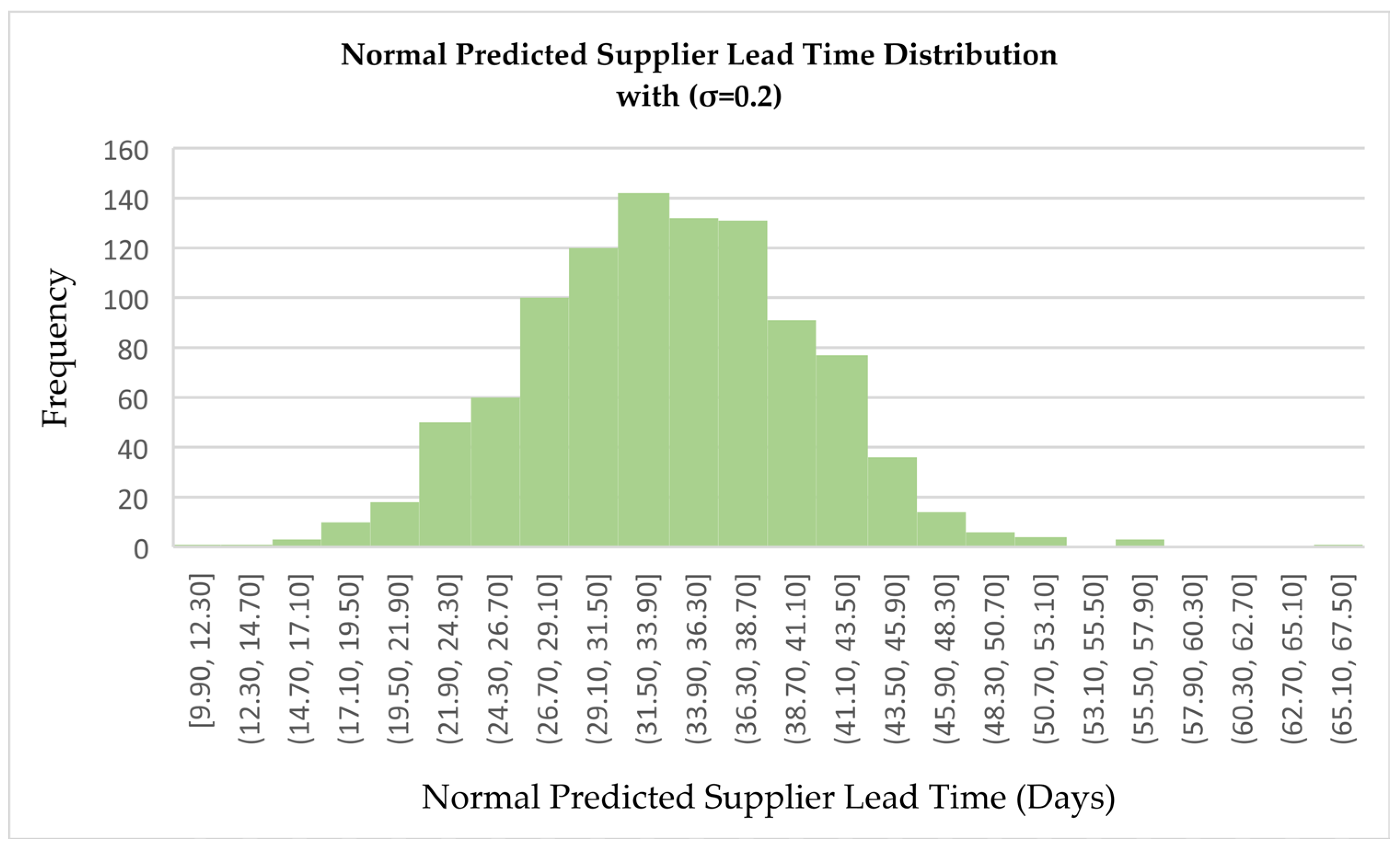
This subsection presents a comparative analysis of supplier lead times predicted under low-variability conditions (σ = 0.2). Different distribution models, including log-normal (Figure 3), normal (Figure 4), and IoT-adjusted log-normal (Figure 5), are examined to understand their behavior and accuracy. The comparison highlights how the choice of distribution and the integration of IoT technologies impact the prediction of delays and the overall reliability of the supply chain.

a.

Log-Normal Predicted Supplier Lead Time Distribution (σ = 0.2)

• Interpretations:

The distribution is right-skewed, typical of a log-normal shape. Most predicted supplier lead times are concentrated between approximately 26 and 40 days, indicating a relatively narrow and consistent range. The peak (mode) occurs around 31 to 33 days, showing the most frequent delivery timeframe. There is a long right tail, indicating a small probability of longer lead times. This reflects a realistic pattern for supplier lead times under low variability, where occasional delays are possible but most deliveries fall within a predictable window.

b.

Normal Predicted Supplier Lead Time Distribution (σ = 0.2)

• Interpretations:

The distribution is symmetric around the mean, which is approximately 31 to 33 days. Predicted lead times are spread equally on both sides of the mean, reflecting the typical bell shape of a normal distribution. However, the normal distribution assumes the possibility of negative values, which is unrealistic for modeling lead times, as delivery times cannot be less than zero. While the variability is balanced, this symmetry does not accurately reflect real-world lead time behavior, which is often skewed due to occasional disruptions. As such, the normal distribution serves as a theoretical benchmark, but it has clear limitations when applied to practical supply chain modeling.

c.

IoT-Adjusted Log-Normal Predicted Supplier Lead Time Distribution (σ = 0.2)

• Interpretations:

The distribution remains right-skewed but becomes sharper around the peak, indicating a more concentrated range of predicted lead times. The peak is more pronounced around 33 to 35 days, reflecting increased accuracy in forecasted delivery times. The decline towards longer lead times is steeper compared to the standard log-normal distribution, suggesting a reduced likelihood of extreme delays. IoT adjustments have improved responsiveness and helped reduce lead time uncertainty, making predictions more reliable. This demonstrates the positive impact of IoT technologies on supplier performance and overall supply chain reliability.

5.1.2. Comparison of Predicted Supplier Lead Time Distributions Under a Medium-Variability Scenario

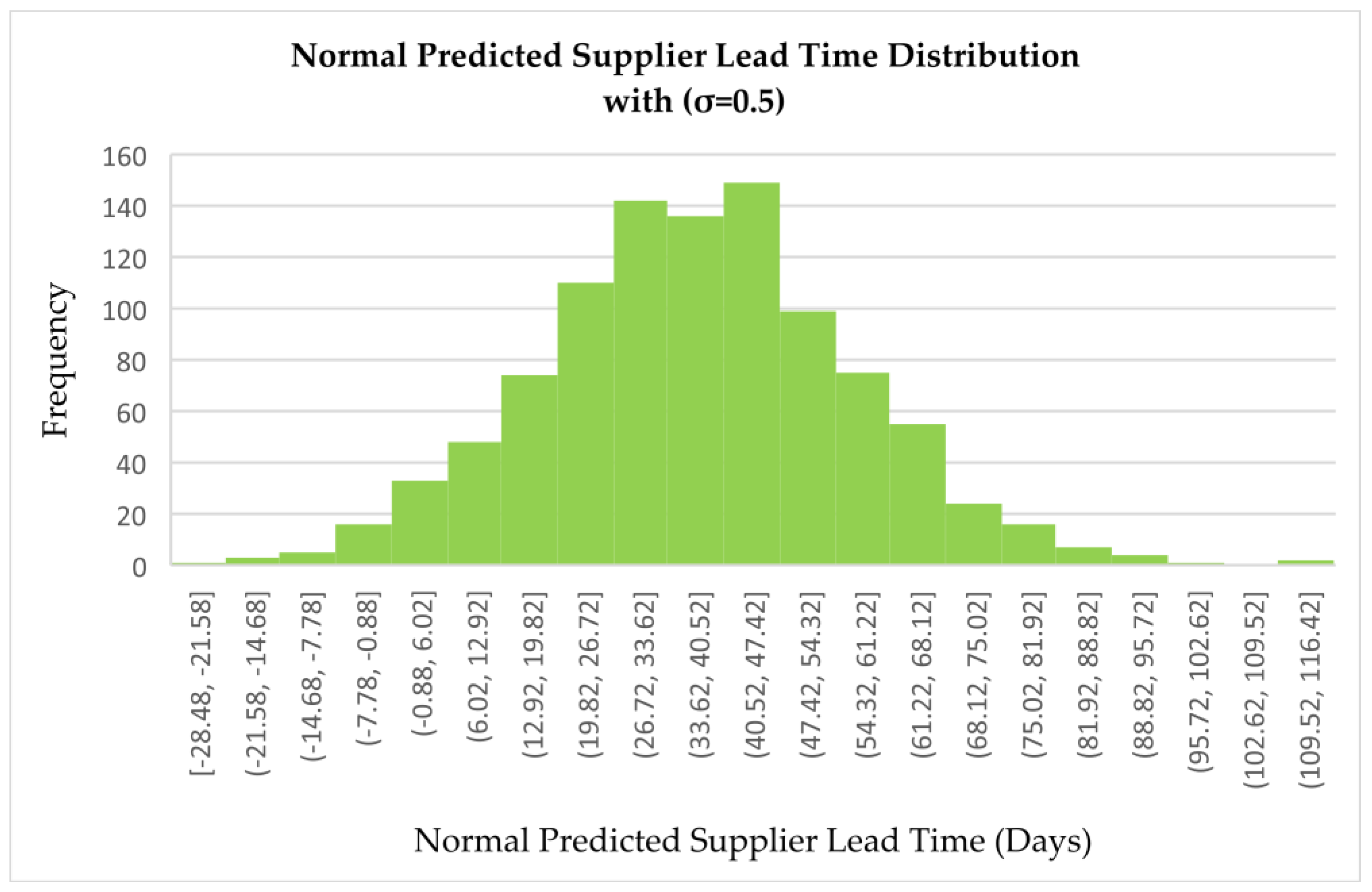
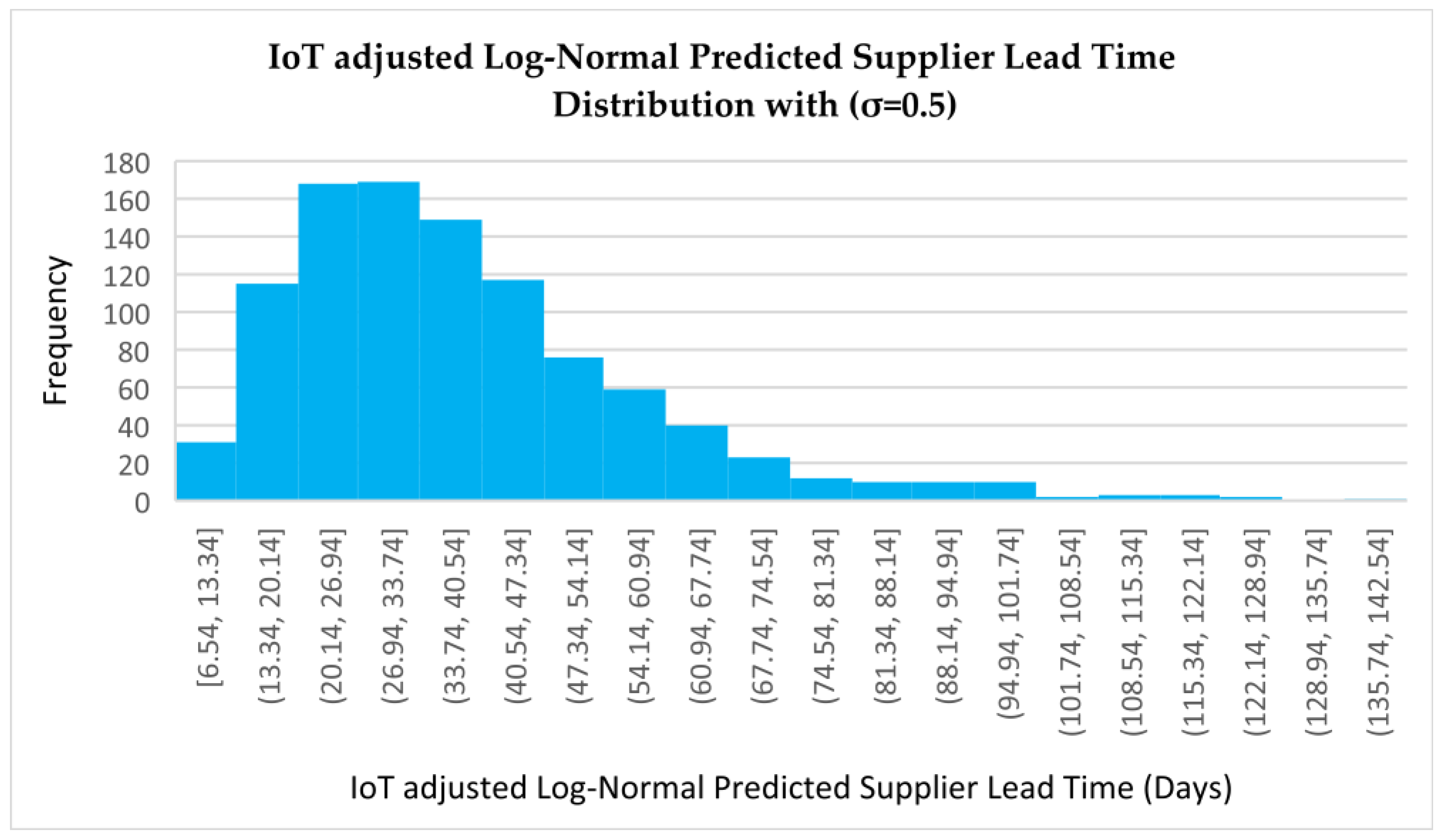
In this subsection, we analyze the predicted supplier lead times under medium-variability conditions (σ = 0.5). By comparing the behavior of log-normal (Figure 6), normal (Figure 7), and IoT-adjusted (Figure 8) distributions, we aim to highlight how increased variability affects the accuracy of lead time predictions and the overall performance of the supply chain. The results provide insights into the importance of selecting appropriate distribution models and leveraging digital technologies to maintain supply chain resilience even when uncertainty rises.

a.

Log-Normal Predicted Supplier Lead Time Distribution (σ = 0.5)

• Interpretations:

The distribution is positively skewed, typical of a log-normal distribution, with supplier lead times ranging from 6.5 days to beyond 138.5 days. The highest frequency is observed in the intervals (19.7, 26.3] and (26.3, 32.9], with approximately 165 and 160 occurrences, respectively. This indicates that the majority of supplier lead times lie between 19 and 33 days. The peak is therefore centered around 19 to 26 days, representing the most frequent delivery range. A long upper tail is visible, with low-frequency values in higher intervals such as (85.7, 92.3], (105.5, 112.1], and (131.9, 138.5], suggesting that suppliers may experience rare but significant delays. The overall pattern reflects a scenario where most suppliers deliver within a predictable timeframe, but a few outliers cause substantial variation in lead times. This reflects a realistic behavior of supplier performance in industrial settings, where short to moderate delays are common, and longer delays occur infrequently but can have a significant impact.

b.

Normal Predicted Supplier Lead Time Distribution (σ = 0.5)

• Interpretations:

The distribution is symmetric and bell-shaped, characteristic of a normal distribution, with lead time values ranging approximately from -28.48 to 116.42 days. However, it is important to note that negative values are unrealistic in practical supplier contexts. The peak is observed around the intervals (40.52, 47.42] and (26.72, 33.62], with each containing approximately 140 to 150 observations, indicating that most supplier lead times are centered between 26 and 47 days. The distribution spreads evenly on both sides of the peak, with decreasing frequencies toward the tails, as shown by intervals such as (88.82, 95.72], which have fewer than 10 occurrences. The presence of negative lead time bins, such as [-28.48, -21.58], is a mathematical artifact of the normal distribution and highlights its unsuitability for modeling inherently non-negative variables like lead times.

This distribution implies predictable and balanced supplier behavior, but it lacks realism in representing the delays and variability typically encountered in real-world supply chains. It suggests an equal probability of having lead times shorter or longer than the average, which is often unrealistic for practical modeling. In reality, lead times are rarely shorter than expected and often exhibit right-skewed behavior. Moreover, the normal distribution allows for lower and higher values with similar likelihoods around the mean, which can misrepresent the actual risk of extreme delays.

c.

IoT-Adjusted Log-Normal Predicted Supplier Lead Time Distribution (σ = 0.5)

• Interpretations:

The distribution remains positively skewed, but with a slightly broader spread compared to the initial log-normal distribution. The predicted supplier lead times now range from 6.54 days to 142.54 days. This reflects the increased variability introduced by IoT-based real-time adjustments, where lead time predictions evolve dynamically based on live operational data. The peak of the distribution occurs in the intervals (20.14, 26.94] and (26.94, 33.74], each showing approximately 170 occurrences, indicating that most supplier lead times are still concentrated between 20 and 34 days. The peak remains around 20–26 days, but there is a noticeable extension in both directions, particularly in the upper tail—as seen in intervals like (108.94, 115.94] and (135.74, 142.54]—which suggests occasional significant increases in lead time due to unforeseen events or disruptions.

5.1.3. Comparison of Predicted Supplier Lead Time Distributions Under a High-Variability Scenario

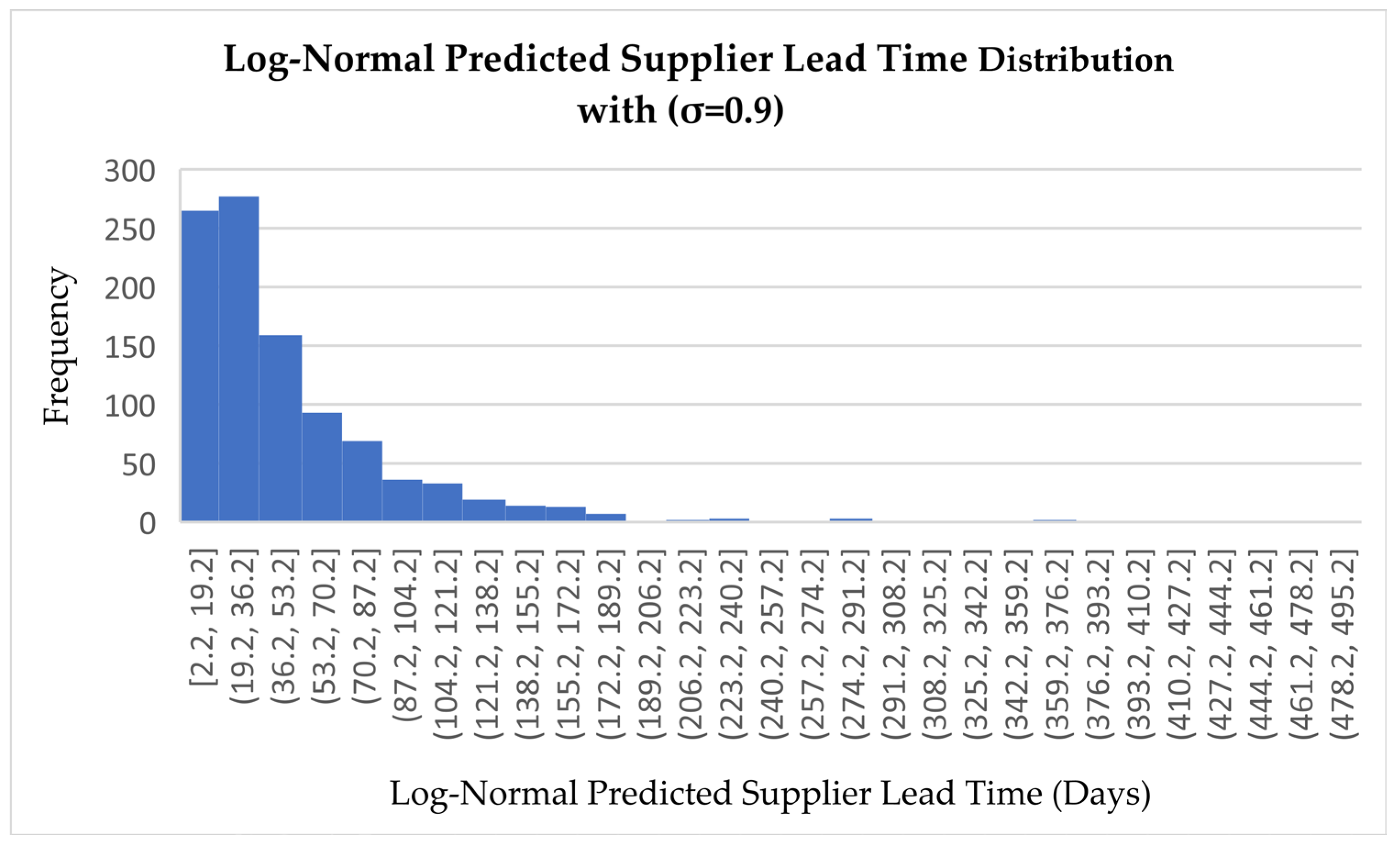
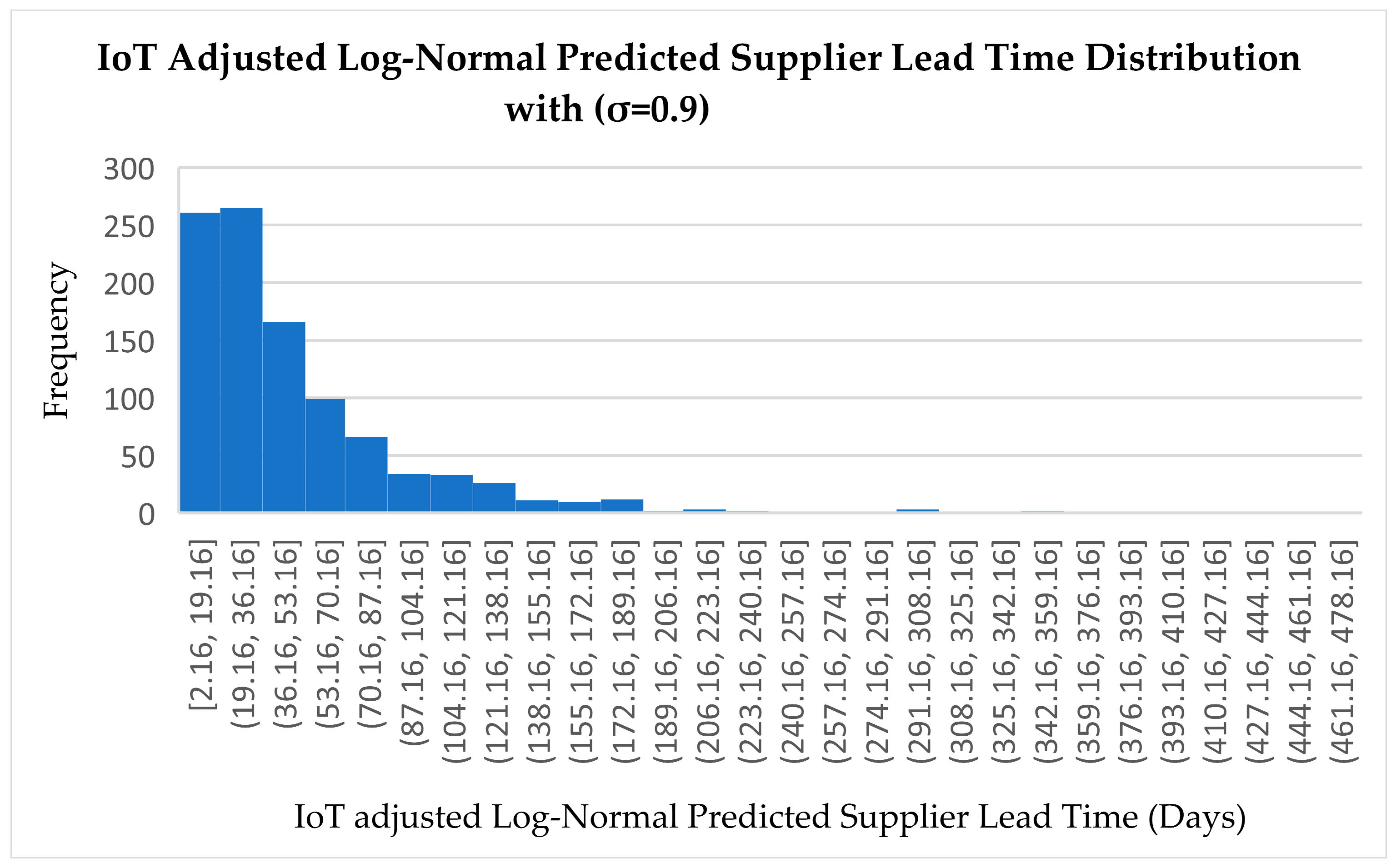
This subsection examines the predicted supplier lead times in a high-variability context (σ = 0.9). The comparison between log-normal (Figure 9), normal (Figure 10), and IoT-adjusted (Figure 11) distributions allows us to observe how greater uncertainty amplifies deviations and risks in lead time estimation. The analysis underscores the critical role of robust predictive models and the value of IoT-driven adjustments in mitigating the effects of extreme variability on supply chain performance.

a.

Log-Normal Predicted Supplier Lead Time Distribution (σ = 0.9)

• Interpretations:

The distribution is right-skewed, which is a typical feature of the log-normal model, with lead time values ranging from approximately 2.21 to 495.2 days. The majority of supplier lead times are concentrated in the interval (2.21, 36.2], with over 260 occurrences, suggesting that most deliveries occur within a timely and predictable range. However, there is a long tail extending toward very high lead times, reaching up to 495 days, which captures the possibility of rare but significant supplier delays. Importantly, the absence of negative values in the distribution makes the model more realistic for operational applications, unlike the normal distribution, which permits mathematically possible but practically implausible negative lead times.

b.

Normal Predicted Supplier Lead Time Distribution (σ = 0.9)

• Interpretations:

The distribution is symmetric and bell-shaped, with supplier lead times ranging from approximately –116.5 to 219.5 days. The peak is observed between the intervals (43.54, 51.54], with around 65 occurrences in the central bins, indicating that most predicted values cluster near the mean. Frequencies decline symmetrically on both sides of the peak, consistent with the expected behavior of a normal distribution. However, the appearance of negative lead time values in several bins such as [-116.5, -92.51] is unrealistic and highlights a critical limitation of the model. While the normal distribution presents a balanced and mathematically elegant pattern, it lacks practical relevance in this context due to its inability to accurately model non-negative variables like supplier lead time.

c.

IoT-Adjusted Log-Normal Predicted Supplier Lead Time Distribution (σ = 0.9)

• Interpretations:

This distribution retains the right-skewed shape typical of the log-normal model, but with a tighter concentration around lower lead times, ranging from 2.16 to 461.16 days. The highest density occurs in the interval (19.16, 36.16], with nearly 270 occurrences, indicating a strong clustering of efficient supplier responses. The tail is significantly thinner than in the standard log-normal distribution, suggesting better control over extreme delays, likely enabled by IoT-based monitoring and early warning systems. As expected, no negative lead times appear, preserving the model’s realism and operational relevance. Compared to both the standard log-normal and normal distributions, this model demonstrates superior performance, characterized by a tighter spread, fewer outliers, and a more accurate reflection of supplier behavior. The integration of IoT enhances predictability, responsiveness, and reliability, making this model particularly effective for smart supply chain management.

5.1.4. Comparison of Predicted Supplier Lead Time Distributions Under a Very-High-Variability Scenario

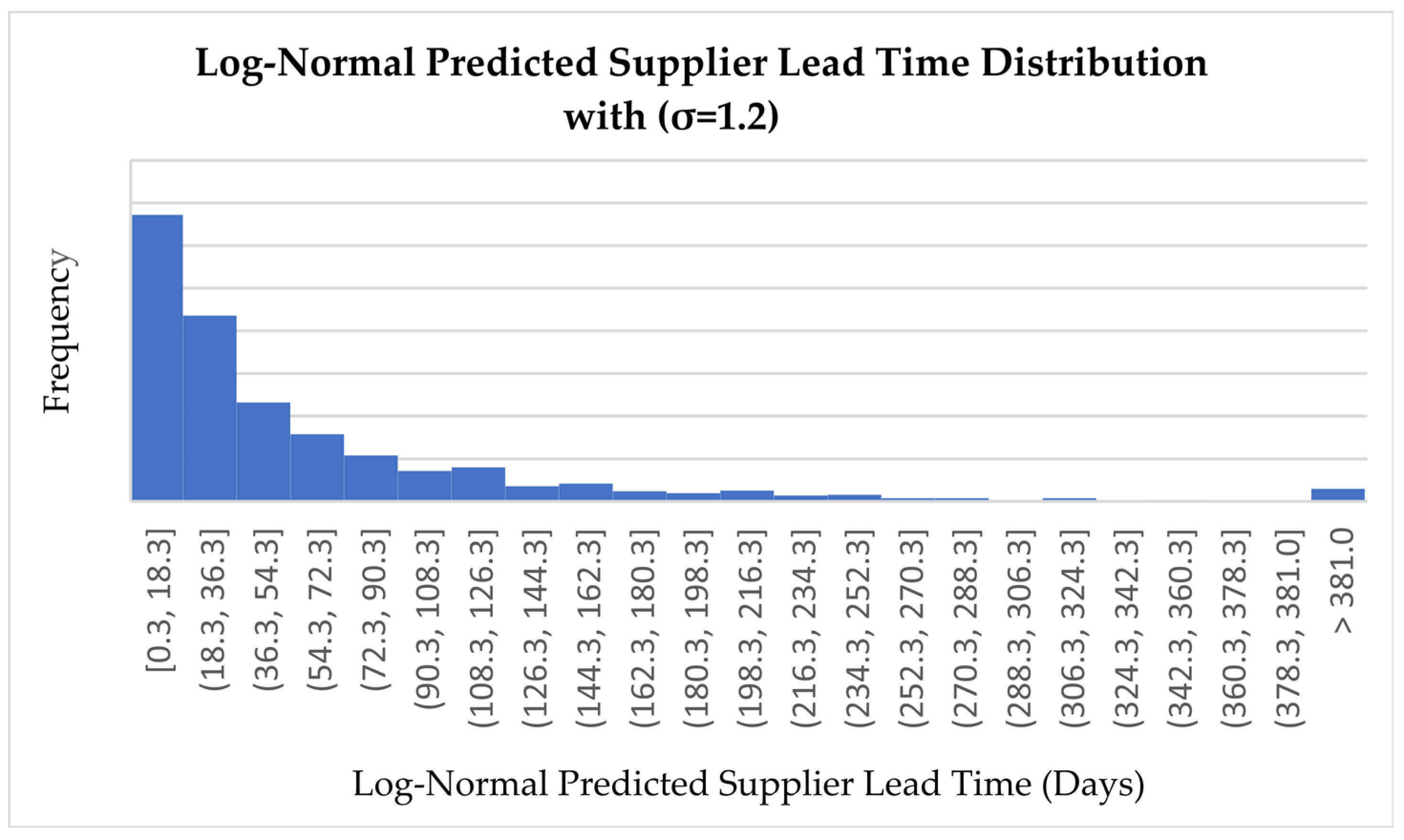
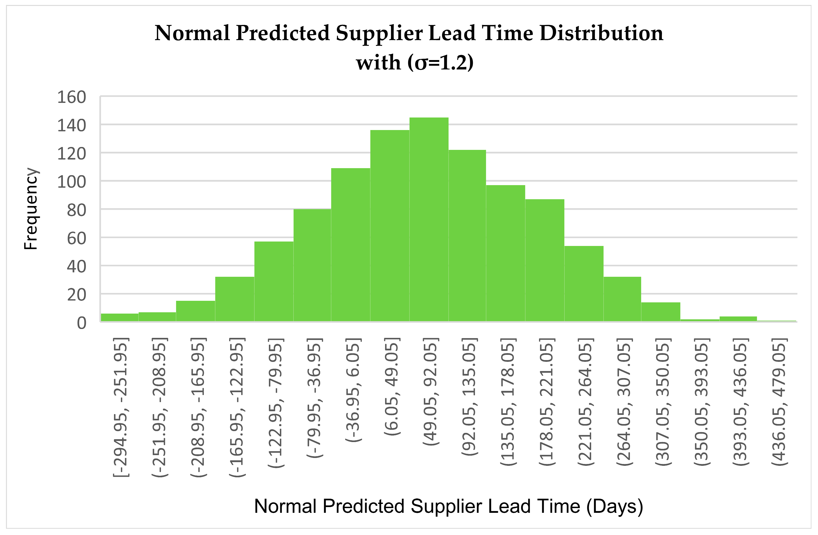
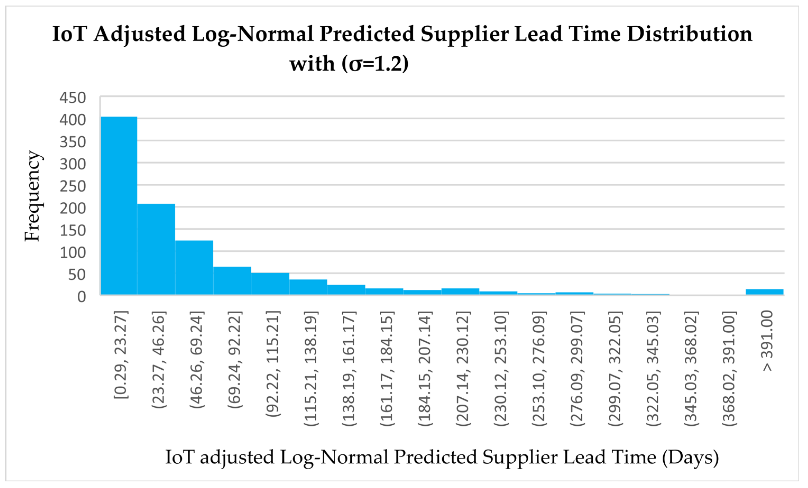
In this subsection, we analyze the predicted supplier lead times under very-high-variability conditions (σ = 1.2). By comparing the behavior of log-normal (Figure 12), normal (Figure 13), and IoT-adjusted log-normal (Figure 14) distributions, we aim to highlight how extreme variability impacts the accuracy of lead time predictions and the robustness of the supply chain. The results provide insights into the value of integrating dynamic IoT adjustments with statistical models to enhance decision-making and maintain performance under significant uncertainty.

a.

Log-Normal Predicted Supplier Lead Time Distribution (σ = 1.2)

• Interpretations:

The distribution produced by the log-normal model under extreme variability (σ = 1.2) is strongly right-skewed, as expected for this type of distribution. The majority of predicted supplier lead times fall between 0 and 54 days, with the highest frequency concentrated in the interval [0.3, 18.3], reaching nearly 340 occurrences. Beyond this range, the frequency declines rapidly, but a long upper tail extends past 381 days, indicating the model’s ability to represent rare but severe supplier delays. This shape realistically reflects actual supplier performance under extreme conditions—where most deliveries occur within a standard range, but exceptional disruptions can result in significant lead time extensions.

b.

Normal Predicted Supplier Lead Time Distribution (σ = 1.2)

• Interpretations:

The distribution generated using the normal model is symmetric and bell-shaped, with lead time values ranging from approximately -294.95 to over 436 days. The peak is centered between 49.05 and 92.05 days, with values distributed evenly on both sides. However, the presence of negative lead time values is a major drawback, as it violates the non-negative nature of real-world delivery times. This reveals a fundamental limitation of the normal distribution in high-variability supply chain modeling: while it provides a mathematically balanced structure, it fails to capture the inherent asymmetry and risk of extreme delays, making it less suitable for practical forecasting in EtO environments facing severe disruptions.

c.

IoT-Adjusted Log-Normal Predicted Supplier Lead Time Distribution (σ = 1.2)

• Interpretations:

The IoT-adjusted log-normal model maintains a right-skewed structure but shows a tighter concentration of predicted lead times in the lower intervals. The highest frequency appears in the range [0.29, 23.27], with nearly 400 occurrences, indicating strong clustering of efficient supplier responses. Compared to the standard log-normal model, the tail is less pronounced, although some extreme delays still exist beyond 391 days. This reduction in tail weight and variability suggests that the IoT-based dynamic adjustments have enhanced prediction accuracy and responsiveness. The resulting distribution provides a more operationally realistic and resilient tool, particularly well suited to smart supply chain management under conditions of extreme uncertainty.

5.2. Summary of Lead Time Distribution Interpretations Across Variability Scenarios

The comparative analysis of supplier lead time distributions across low- (σ = 0.2), medium- (σ = 0.5), high- (σ = 0.9), and very-high- (σ = 1.2) variability scenarios reveals consistent limitations in traditional prediction models and highlights the increasing value of the proposed IoT-adjusted log-normal approach. Under low variability, the log-normal distribution realistically captures mild asymmetry and rare delays, while the normal model fails to reflect operational reality due to its symmetry and inclusion of negative values. The IoT-adjusted log-normal model improves further by tightening the distribution around the peak and reducing uncertainty, showing the benefits of dynamic real-time responsiveness.

As variability increases to medium, the log-normal model maintains its robustness in modeling skewness and outliers, whereas the normal model begins to show greater deviation from real-world behavior, especially due to its balanced shape and unrealistic assumption of symmetrical error distribution. The IoT-enhanced log-normal distribution adapts to the wider spread by leveraging live data, improving accuracy while still capturing variability.

In the high-variability scenario, the shortcomings of the normal distribution become more pronounced, with frequent implausible negative lead times and poor handling of extreme values. The log-normal distribution still performs reasonably well but lacks adaptability. In contrast, the IoT-adjusted model significantly reduces the frequency of outliers and concentrates predictions in a more operationally relevant range, confirming its practical advantage.

Finally, under very high variability (σ = 1.2)—which simulates extreme disruptions such as pandemics or geopolitical shocks—the normal model proves unsuitable due to its inability to capture right-skewed, non-negative, and erratic supplier behavior. The log-normal model, while structurally appropriate, shows a long tail and limited control over extreme delays. The IoT-adjusted log-normal model again proves the most effective, demonstrating tighter clustering, reduced tail weight, and enhanced prediction accuracy under extreme uncertainty.

Overall, the analysis confirms that the IoT-enhanced log-normal model offers the most realistic, accurate, and resilient predictive performance across all scenarios. It aligns with the operational realities of Engineer-to-Order (EtO) supply chains, where uncertainty, customization, and responsiveness are critical. This model provides a robust decision-support tool for managing risk and improving lead time reliability in both stable and highly disruptive environments.

5.3. Statistical Validation of the Proposed Approach

To evaluate the effectiveness and robustness of the proposed log-normal distribution model for predicting supplier lead times in an EtO environment, Monte Carlo simulations were conducted under three variability scenarios: low variability (σ = 0.2), medium variability (σ = 0.5), and high variability (σ = 0.9). The performance of the log-normal predicted lead time, normal predicted lead time, and IoT-adjusted log-normal predicted lead time was compared using two statistical metrics: the Mean Absolute Error (MAE) and Root Mean Square Error (RMSE). These two metrics are widely used in statistical validation, providing insight into both the average deviation of predictions and the impact of larger errors.

The MAE is defined as follows:

$$MAE={\displaystyle \frac{1}{n}} \sum _{i=1}^n\left|y_i-{\widehat{y}}_i\right|$$

(7)

where $y_i$ represents the actual lead time, ${\widehat{y}}_i$ is the predicted lead time, and n is the total number of observations. A lower MAE indicates that the predictions are, on average, closer to the observed values.

The RMSE, which places greater weight on large errors, is defined as follows:

$$\mathrm{R}\mathrm{M}\mathrm{S}\mathrm{E}=\sqrt{{\displaystyle \frac{1}{n}} \sum _{i=1}^n(y_i-{{\widehat{y}}_i)}^2}$$

(8)

A lower RMSE suggests that extreme deviations are minimized, making the model more robust in capturing variability.

5.4. Interpretations of Prediction Accuracy Across Variability Scenarios

Table 1. Comparison of lead time prediction accuracy across variability scenarios.

Scenario	Model	MAE	RMSE	Comments
Low variability	Normal distribution	3.57	4.12	Baseline with normal distribution
	Log-normal distribution	2.44	3.36	Improved accuracy due to better modeling of skewness
	IoT-adjusted log-normal distribution	1.78	3.91	Best accuracy by integrating real-time adjustment factors
Medium variability	Normal distribution	5.89	7.22	Degradation in accuracy with normal distribution
	Log-normal distribution	3.87	5.46	Maintains robustness against increased variability
	IoT-adjusted log-normal distribution	2.85	5.75	Enhances lead time accuracy with dynamic data inputs
High variability	Normal distribution	8.33	10.25	Significant errors due to inability to handle outliers
	Log-normal distribution	6.14	8.87	Remains reliable even in volatile supply environments
	IoT-adjusted log-normal distribution	4.91	9.08	MAE improves, RMSE sensitive to extreme delays
Very high variability	Normal distribution	11.54	13.90	Likely unsuitable due to unrealistic predictions and frequent negative values
	Log-normal distribution	8.91	12.21	Handles skewness but still prone to extreme delay outliers
	IoT-adjusted log-normal distribution	6.83	10.47	Best performance under crisis-level conditions; reduced tail risk

compares the performance of lead time prediction models across four levels of supply chain variability: low, medium, high, and very high.

Under low variability (σ = 0.2), all models provide acceptable results, but the log-normal distribution outperforms the normal distribution by better modeling right-skewed data. The IoT-adjusted log-normal model achieves the best MAE, demonstrating its capacity to refine forecasts through real-time responsiveness, even in stable conditions.

In the medium-variability scenario (σ = 0.5), prediction errors increase for all models, particularly for the normal distribution. The log-normal model remains robust, and the IoT-adjusted variant further enhances accuracy by dynamically responding to operational signals, achieving the lowest MAE in this category.

Under high variability (σ = 0.9), typical of volatile supply environments, the normal model’s prediction errors become significant, especially in RMSE. The log-normal model continues to perform reliably, while the IoT-adjusted log-normal model demonstrates improved average prediction accuracy. However, its RMSE slightly increases due to the model’s sensitivity to rare but extreme lead time disruptions. These outliers, although infrequent, exert a disproportionate influence on the RMSE value, highlighting the metric’s emphasis on large deviations. This distinction explains why RMSE and MAE may diverge under high variability conditions and underscores the importance of using both metrics for a comprehensive performance evaluation.

In the very-high-variability scenario (σ = 1.2)—representing extreme disruptions such as pandemics or geopolitical shocks—the normal model proves unsuitable due to frequent unrealistic values, including negative lead times. The log-normal model handles the skewness better but still reflects the influence of rare extreme delays. The IoT-enhanced model outperforms all others, achieving the lowest MAE and substantially reducing RMSE, confirming its robustness and adaptability under severe uncertainty. This validates the model’s effectiveness for real-world EtO supply chains facing high levels of disruption.

In summary, the comparative simulation of four lead time variability scenarios—ranging from low to very high—demonstrated that traditional prediction models based on normal distribution are inadequate for capturing the non-linear and right-skewed nature of lead times in EtO environments. The log-normal model offered a more accurate and statistically appropriate baseline across all levels of variability. Most notably, the proposed IoT-adjusted log-normal model consistently achieved the lowest MAE values, indicating superior average prediction accuracy, adaptability, and resilience—particularly under high uncertainty. These findings validate the effectiveness of integrating probabilistic modeling with dynamic IoT signals for lead time forecasting in complex, customized supply chains.

These results provide a strong foundation for a deeper examination of the broader implications of this study, which are addressed in the following section.

6. Discussion

Building on the simulation outcomes across varying levels of lead time variability, this section explores the broader significance of the findings from theoretical, managerial, and practical perspectives. It discusses how the proposed framework advances current knowledge, supports decision-making in EtO supply chains, and opens pathways for future research and practical implementation in real-world settings.

6.1. Implications for Theory

This study contributes to the theoretical advancement of supply chain modeling in EtO environments by addressing the limitations of traditional symmetric lead time distributions. Specifically, it applies the log-normal distribution to model the stochastic behavior of supplier lead times, offering a more realistic representation of delays typically observed in customized production settings. By doing so, it extends the current body of knowledge in stochastic modeling and highlights the relevance of asymmetrical distributions in high-variability environments. Furthermore, the research introduces a hybrid conceptual framework that integrates probabilistic modeling, Monte Carlo simulation, and IoT-enabled responsiveness. This interdisciplinary approach bridges gaps between supply chain analytics, industrial engineering, and digital manufacturing, contributing to the growing discourse on Industry 4.0. It also offers a theoretical foundation for developing adaptive, data-driven forecasting models in contexts where historical data are scarce or unreliable—a common challenge in EtO systems. Ultimately, this work enhances the theoretical understanding of how real-time technologies and uncertainty modeling can coalesce to inform predictive decision-making in dynamic supply networks.

6.2. Implications for Managers and Policymakers

From a practical perspective, the study provides a simulation-based decision-support model tailored to the unique challenges of EtO supply chains. This model enables managers to improve the accuracy of lead time predictions even in environments with incomplete or inconsistent data—a critical capability in highly customized production systems. By emphasizing the formation of long-term partnerships with suppliers of customized raw materials, the study highlights the operational benefits of establishing continuous data exchange channels, which allow for real-time monitoring and adjustment of procurement plans. Additionally, the proposed model is designed to be compatible with intelligent planning tools and digital twins, offering a pathway for integration into advanced supply chain management platforms. For managers, this means better visibility of potential lead time risks, more responsive scheduling, and enhanced resilience against disruptions. For policymakers, the findings underscore the importance of supporting digital infrastructure and incentivizing collaborative supplier relationships as part of broader industrial innovation strategies. Together, these practical insights align with the goals of smart manufacturing and supply chain resilience in Industry 4.0 contexts.

While the integration of IoT-based adjustments offers significant potential to enhance the accuracy and adaptability of lead time prediction models, several practical challenges must be taken into account when considering real-world implementation. First, data privacy and cybersecurity are critical concerns, especially when sensitive operational data is transmitted across organizational boundaries. Ensuring secure communication protocols, end-to-end encryption, strict access control mechanisms, and adherence to relevant data protection standards such as GDPR and ISO/IEC 27001 is essential. Additionally, clear data governance policies must be established between supply chain partners to define data ownership, usage rights, and responsibilities, thereby protecting sensitive data and building trust among stakeholders. Second, the reliability and maintenance of sensor devices can affect the accuracy and consistency of real-time data, particularly in environments exposed to harsh operational conditions. Third, the cost of deploying IoT infrastructure—including sensors, data transmission systems, and analytics platforms—can represent a substantial investment, especially for small or medium-sized enterprises. These considerations highlight the importance of strategic planning, supplier collaboration, and technical support when integrating IoT into supply chain prediction systems. Addressing these challenges is essential to ensure the scalability, trustworthiness, and long-term sustainability of IoT-enabled forecasting solutions in EtO environments.

6.3. Limitations of the Study and Future Research Directions

However, certain limitations must be acknowledged. The model relies on synthetic data due to the lack of real historical lead time records, and the adjustment factors from IoT were generated through simulation rather than actual sensor inputs. Moreover, the framework is currently limited to single-supplier scenarios and does not account for complexities such as multi-tier supply networks or capacity constraints.

To overcome these limitations, future work should focus on validating the model with real industrial data and integrating real-time IoT sensor streams to enable dynamic lead time adjustment. Improving the framework with advanced machine learning methods could enhance the accuracy of real-time predictions. Additionally, expanding the model to include multi-supplier scenarios, capacity constraints, and alternative sourcing strategies would increase its robustness and relevance. Developing a user-friendly decision-support tool, with visualization dashboards and integrated optimization algorithms, would further help in turning predictive insights into practical, strategic actions.

7. Conclusions

This paper proposed an integrated framework for predicting supplier lead times in EtO supply chains by combining log-normal probabilistic modeling with IoT-based real-time adjustment factors. The findings demonstrate that the log-normal distribution more accurately captures the non-negative and right-skewed nature of lead time variability than the commonly used normal distribution. Monte Carlo simulations across multiple variability scenarios showed that the model significantly improves prediction accuracy and supply chain responsiveness, particularly when enriched with simulated IoT-derived adjustments.

The significance of these findings lies in the framework’s ability to bridge the gap between statistical modeling and real-time operational feedback. This contributes to more resilient and agile supply chain planning, especially in complex, customized production environments. The model’s application to EtO contexts suggests broader adaptability for industries facing similar uncertainty and variability. This research lays a foundation for practical implementation in digital supply chains and opens up future research avenues, such as sensitivity analyses of distribution parameters and integration with digital twin systems. As organizations increasingly seek supply chain resilience, models like the one proposed here can support both operational decisions and strategic sourcing policies.