Efficient Simulation Algorithm and Heuristic Local Optimization Approach for Multiproduct Pipeline Networks

Abstract

Background: Managing multiproduct pipeline systems is a complex task of critical importance in the petroleum industry. Experts frequently rely on simulation tools to design and validate pumping operation schedules. However, existing tools are often problem-specific and too slow to be effectively used for optimization purposes. Methods: In this paper, a new scheduling model is introduced, which inherently eliminates all conflicts except for tank overflows and underflows. A Discrete-Event Simulation algorithm was developed, capable of handling mesh-like pipeline topologies, reverse flows, and interface tracking. The computational performance of the new method is demonstrated using three local search-based optimization variants, including a simulated annealing metaheuristic. Results: A case study was made involving four problems, with 4–6 sites and 5–7 products in mesh-like and straight topologies, respectively, and a large-scale instance. Scheduling horizons of 2–28 days were used. The proposed simulation algorithm significantly outperforms a prior approach in speed, and the optimization algorithms effectively converged to feasible, high-quality schedules for most instances. Conclusions: This paper proposes a novel simulation technique for multiproduct pipeline scheduling along with three local search algorithm variants that demonstrate optimization capabilities.

1. Introduction

Multiproduct pipelines are widely used for transporting liquids over long distances. The most notable applications are from the petroleum industry, where the liquids are refined petroleum products. Pipelines are relatively cheap, safe, and less prone to unexpected events than other modes of transportation such as road, rail, or barges [1]. A multiproduct pipeline segment is characterized by a load of constant total volume. Product batches inside pipes travel in plugs next to each other that are in direct contact. Since liquids are practically incompressible, pumping products into a pipeline network requires that the same amount be simultaneously pushed out at a remote site. That amount may consist of a different product that was pumped hours or days earlier, possibly at a different origin site. One has to take into account the tank volumes at sites, which are influenced by not only pumping operations but planned production and deliveries. Moreover, a good schedule should incur minimal costs, which are related to factors like interface forming between different product batches, turning pumps on and off, and energy consumption. Therefore, constructing an optimal schedule for the pipeline is a challenging task and has also proven to be NP-hard under simple assumptions [2].

A comprehensive review on the wide range of recent approaches is provided by Sidki et al. [3]. Proposed optimization models generally focus on some well-specified problem class regarding network topology, tank management, objective, optimization method, and other circumstances. Some problem features that are less frequently addressed in the literature are arbitrary network topologies, non-trivial flow rates, and reverse flows. There are some features which are in focus but hard to model, such as batch splitting and interfaces between product batches. If a particular use case for a given pipeline is to be addressed, existing methods are not applicable directly, because the needs and restrictions are unique in each real-world case.

Simulation is a commonly used method for supporting management of complex systems, including pipeline networks. A planned schedule, especially when created by humans, is usually verified by some kind of computational algorithm. There is a significant difference between the simulation of a single schedule or a few schedules that were designed and adjusted manually and the simulation of a very large number of schedules as part of a search space exploration, as frequently performed by optimization algorithms. For this reason, simulators designed to aid manual work [4] tend to focus on the full detail of the process, including data that are not always relevant and therefore too slow to be effectively used in optimization. Nevertheless, simulation tools have been used as part of optimization [5], but these usages are very specific to a given problem. Enterprise simulator software tools also exist [6], which are tailored to provide full detail of a particular process. Since these tools are also aimed at verifying a single system or plan, their use in optimization is similarly limited.

The goal of the present work is to provide a new problem formulation along with a simulation technique for multiproduct pipeline scheduling. A formal problem definition is given, and a new algorithm is proposed that simulates a given schedule, testing it for feasibility while calculating useful quality measures. By employing aggregate tanks and considering only relevant system data and the efficient management of events, the new algorithm has low computational needs. Moreover, the technique naturally supports an arbitrary pipeline network topology, reversed flows, batch splitting, and the precise calculation of interfaces.

A key idea in the new algorithm design is that most typical contradictions and infeasible situations are eliminated. The only form of infeasibility comes from minimum and maximum tank levels being violated. This kind of infeasibility, as this work will show, can be removed by successive small incremental changes that can be part of the optimization procedure itself.

For this reason, the simulation technique is demonstrated via three optimization algorithms. These are all based on the local improvement of an existing schedule, accepting a neighbor if it has better fitness. The first algorithm is exhaustive under a given set of decisions to make. The second algorithm is more dynamic in improving a solution and also looks ahead for infeasibility. The third algorithm is obtained from the second, by adding a simulated annealing metaheuristic. The algorithms are demonstrated on two moderate pipeline networks. Computational results demonstrate the effectiveness of these algorithms for finding feasible schedules and improving the quality of already feasible schedules. Our experience with these methods is detailed in this paper. The simulation technique is shown to offer a very fast evaluation of a given schedule.

The rest of the paper is structured as follows. A literature review is presented in Section 2. The problem formulation and the proposed simulation technique and optimization algorithms are in Section 3. Computational results for a case study can be found in Section 4, and the work is concluded in Section 5.

2. Literature Review

Several approaches have been proposed for the management of multiproduct pipeline networks. Most are optimization models, and there are some results specific to simulations. These approaches are presented here based on key features. At the end of each subsection, there is a brief explanation on how these features influenced the present work.

2.1. Network Layout

One of the most important aspects of pipeline scheduling is the network layout. The following layouts, ordered from the simplest to the most general, have been considered in the literature:

• Straight pipelines,
• Tree-like pipeline networks,
• Mesh-like or arbitrary pipeline networks.

Furthermore, the allowed flow directions are a key property of the network layout. In some works, pumping operations originate from a single station, while in others, intermediate nodes can also serve as pumping sources. Also, some works consider unidirectional pipes, while others allow reversed flow in bidirectional pipes, a practice also referred to as backtransport.

Straight pipeline networks are characterized by a starting source station (e.g., port or refinery) and several stations for product delivery along the pipeline with no branches. Such systems may model the backbone of a supply chain. Straight networks represent the most common layout among those studied in the context of multiproduct pipeline scheduling [3]. Early approaches used mathematical programming models for straight networks and were able to solve real-world case studies with a few nodes [7]. It is possible that only the first station serves as a pumping station [8]. Other case studies involve multiple pumping stations [9] and even parallel pumping in cases where the pumping operations are unrelated [10].

Some works have considered a more general tree-like structure. In such networks, there is usually a main, trunk line as for a straight pipeline network and branches starting from some intermediate nodes. These networks naturally encompass a broader range of pipeline configurations, but the models for such networks also have a higher complexity. A good example is the work of Cafaro and Cerdá [11], which is a continuous-time Mixed-Integer Linear Programming (MILP) model, demonstrated on a main case study with eight delivery stations. A more recent work by Mostafaei et al. [1] offers good computational performance, while simultaneously allowing passing flow on the main trunk line and pumping into a branch.

Finally, in a few works, the pipeline networks have a mesh-like or arbitrary layout. These are the most general but the hardest to manage. Boschetto et al. [12] is an example for a mesh-like layout and used a multi-layer decomposition approach for solving large-scale instances, with 14 nodes and a similar number of different products. The framework is of very high complexity and requires key planning decisions as an input. Liao et al. [13] proposed a model for multi-source and multi-destination pipelines aimed at cost minimization, which works for unidirectional pipelines without reverse flows.

As the goal was to provide a general tool, this work targets the less-studied case of mesh-like network layouts while also supporting reverse flows, which is a difficult but real-world oriented combination.

2.2. Model Constraints

Inventory management is a crucial aspect of multiproduct pipeline scheduling. Petroleum products may be stored either in dedicated tanks at storage sites or inside the pipes in the form of plugs. The volumes of pipelines are significant, often comparable to tanks. Meanwhile, there are possible inflows to the system and outflows from the system. The production of a refined petroleum product may provide an inflow of products, e.g., as a consequence of a blending operation. Deliveries to clients can be represented as an outflow. These flows must adhere to the available product quantities and tank capacity constraints.

In some works, inventory management is out of the scope of the model [14]. This can be the case if product batch sizing is decided by experts and the optimization model only considers batch sequencing, routing, and maybe splitting.

When inventory is part of the model, maintaining feasible tank balances poses a modeling challenge. Storage violations can be expressed as an objective function to minimize [5]. Another possibility is rigorously enforcing minimum and maximum levels via constraints [15].

Pumping operations are the most important kind of operations when scheduling pipelines. Therefore, proposed approaches mostly focus on pumping decisions. Some works explicitly consider additional activities related to the management of petroleum products, for example, settling periods for newly produced or received products [16].

Optimization models typically operate at an aggregated scheduling level and utilize aggregate tank capacities. This means that the schedule governs a broader view of material flows, but exact timings and details are often simplified or omitted. Detailed scheduling is difficult to achieve due to the inherent complexity of optimization models, but due to improving modeling and solution techniques, there are some results [17]. It should be noted that in simulations, where the models are not for exploring solutions but rather to check manually constructed schedules, detailed schedules are often a requirement. Some works on simulation may consider actual physical tanks one by one [4]. On the other hand, the lack of simplifications and extra bookkeeping may hinder the use for optimization.

Pumping flow rates determine how much product is pumped into a pipeline per unit time, and can be measured in, e.g., m³/h. Flow rates depend on pumping capacities, the affected pipe segments, and the products currently en route. Flow rates are treated in different ways in related works. Models may simplify the flow rate to a constant value [6,18]. Other works may use product-wise different or non-constant flow rate functions. This may be necessary when significant differences exist between products, or actual flows should otherwise be calculated very precisely. In the model proposed by Zhang et al. [9], only flow rate limits are considered, but piece-wise linear flows are assumed for time windows. The MILP model proposed by Liao et al. [19] relies on a flow rate database of different scenarios. In another related work, flow rate constraints are obtained by pressure control inside the model [20]. Pipeline operators may also use additives to alter the physical properties of products and enhance flow rates [21].

When plugs of different products are pumped next to each other, small amounts inevitably mix, and an interface is formed. This results in product loss that necessitates costly transportation and reprocessing. Therefore, a general goal of pipeline scheduling is to minimize interfaces.

There are different attitudes of published approaches towards interface management. In some cases, interfaces are not in focus and are disregarded in the model [4]. Control of interfaces can possibly be enforced by operational constraints [19]. Since interface forming is also dependent on the products involved, a viable strategy is to simply forbid specifics product pairs to be in contact [22]. Some models mitigate interfaces with a cost penalty [11]. Moreover, interface reprocessing cost can be so significant that it is a possible objective on its own [5]. Interfaces may even be mitigated by inserting small extra plugs in between [5]. If an interface already exists, it is better not kept in pipes for a long time, especially when the flow is stopped, as this may speed up mixing [23]. These examples highlight the depth and complexity involved in managing interfaces effectively.

From the literature examples, it can be seen that some components like interface management are hard to model, but actual needs depend on case. Flow rates may also fall into this category. Therefore, a good approach should support interface tracking and flexible flow rate calculations or be easily extendable to do so. Since a simulation approach is to be presented, that can also check and improve existing schedules, tank inventory management is also a key component of the present work. On the other hand, aggregate tank capacities are sufficient to consider for simulation, since more detailed breakdowns of inventory that some works use may be of little relevance in optimization contexts.

2.3. Objective

There are different goals of optimization models or expert schedulers. A common objective is to minimize operating costs but works differ on what components of costs they focus on, and usually combinations of multiple terms are used. Liao et al. [19] combines pumping costs, representing a quality measure, alongside deviation from demand, which pertains to feasibility. A later work includes a combination of pumping, reverse flow, interface, and other costs [13]. Accumulated idle volume [18] is an example for a special quality measure, which expresses costs associated to pump restarts. The authors in the mentioned works assume constant flow rates.

Another class of approaches have an operational objective. Examples include operational stability quantified by fluctuations of flow rates [14], or deviation between demand and delivery plan [23]. A general observation is that turning pumps on and off incurs extra costs and equipment degradation and might also cause interfaces to expand.

For simulation approaches, incorporating objective evaluation within the simulation process is often more straightforward. Therefore, a good simulator algorithm can be general and flexible in this aspect. This means that a range of different objective calculations should be and can be supported.

2.4. Modeling Techniques

Mathematical programming, and in particular, MILP models, are general and popular tools for optimization. MILP models for multiproduct pipeline scheduling may use discrete or continuous time. Discrete-time models rely on predefining a set of time slots over the time horizon of the schedule. Discrete-time models are simpler to formulate, while still allowing continuous volumes, but their search space is slightly constrained, and the large number of time slots also introduces a computational burden. This was experienced by early works, e.g., Rejowski and Pinto [24], although the obtained models can be improved by some clever constraints [25]. A more recent, monolithic MILP approach using discrete time was reported to be successful for smaller problems with 3–5 delivery stations [26]. Continuous time MILP models [8,11,19] are more general but also harder to formulate and solve.

Either way, standalone MILP models tend to be too large to be solved in real-life instances. For this reason, approaches often use a decomposition scheme to decrease complexity. The work of Boschetto et al. [12] uses layers of assignment, sequencing, simulation, and timing phases. Improvements were later introduced for this large decomposition framework, including a planning phase with an MILP model [27]. The method of Polli et al. [5] uses a heuristic algorithm together with an MILP model. Combinations with other techniques exist, for example, Constraint Logic Programming (CLP) combined with an MILP model [28].

Metaheuristics are another viable class of optimization techniques. Although not guaranteeing an optimal solution, metaheuristics may offer rapid search space exploration and good quality solutions in acceptable time. Chen et al. [14] used Simulated Annealing (SA) for a straight network layout. It should be remarked that their approach included a special space-recursive method for finding an initial solution and tailor-made heuristics to improve existing solutions. Crane et al. [29] is an early application of Genetic Algorithms (GAs) for multiproduct pipeline scheduling. Notably, the authors used a sophisticated award system to guide the search process. A metaheuristic like a GA can be combined with mathematical programming tools and address otherwise difficult model elements like reverse flows [30]. Ribas et al. [31] proposed a micro-genetic algorithm with low population, as part of a hybrid GA-MILP approach. A great advantage of the GA component was the flexibility to generate a set of solutions rather than a single one. Haoran et al. [23] combined the Ant Colony Optimization (ACO) metaheuristic for addressing sequencing decisions with an MILP model to optimize the rest of the decisions. Some approaches use simple heuristic rules for finding good schedules instead. Sasikumar et al. [32] used knowledge-based heuristics to design a system performing in real environment. It is worth noting that the model was revised multiple times during the development procedure before application.

It seems convincing that monolithic MILP models are too expensive in the long term. Heuristic and metaheuristics approaches can be more flexible and scalable, but the aforementioned examples suggest that a clever guidance should be designed for them to work efficiently. Also, these kinds of techniques often require rapid successive evaluation of schedules, which suggests the need for an efficient and general simulation algorithm.

2.5. Simulation Approaches

Simulation refers to the process of determining system behavior under a given scheduling plan. The topic of simulation is very closely related to optimization.

Some optimization techniques already use simulation as part of the procedure [12]. The key is that simulation calculates some details of a solution or part of a solution that would be otherwise difficult or impossible to include in a single optimization model. Meanwhile, an effective simulator is computationally efficient and can be executed for many different instances within acceptable time frames. A good example for this synergy is the work of García-Sánchez et al. [21], which used simulation as part of a tabu search algorithm. Their model works for tree-like networks. A general idea is to use simulation for evaluating a fitness function in a metaheuristic.

A simulator software can be used alone as a design aid tool for experts to manually construct a schedule. Csontos et al. [33] proposed a general purpose simulator, which can handle large-scale mesh-like pipeline networks. In a more recent work [4], the simulator can not only signal an error but can also perform decision-making by fixing schedules. However, several seconds of simulator runtime was reported for a large problem with hundreds of pumping operations, which is too slow for practical use in optimization frameworks.

Many works rely on some already existing simulation framework. Mori et al. [6] used a Discrete-Event Simulation (DES) model and addressed a mesh-like network and reported a 3 min runtime. The DES model of Cafaro et al. [18] was implemented in a known simulation framework to evaluate a few specific scheduling heuristic rules at once. In a more recent result, Strachotová and Dintar [34] developed a simulation framework in an existing environment which could handle mesh-like topology and bidirectional flow, but a limitation of their approach is that some operations, e.g., simultaneous uploading and downloading to a tank, are not allowed. Such approaches often lack the flexibility or speed required for integration into optimization frameworks, which would also require rapid successive simulations.

Overall, existing techniques are tailored to specific problems and are difficult to apply directly, although their key modeling ideas can be useful. There is a clear need for a general purpose simulator that is fast enough to be part of optimization frameworks.

3. Proposed Method

This work presents a new simulation technique for multiproduct pipeline scheduling. Upon the simulation, different variants of a local search optimization algorithm are shown. First, the problem definition is provided. Next, the simulation algorithm and finally the optimization procedures are presented. Some possible extensions of the model are listed in Section 3.4. The algorithm’s implementations with full details, including the case study results in a reproducible form, are available as Supplementary Material attached to this paper.

3.1. Problem Formulation

The general outline for creating a schedule for multiproduct pipelines is shown in Figure 1. The most crucial part of the procedure is when a schedule for simulation is obtained. This can be performed in many possible ways: starting from an empty or random schedule, designing a schedule manually, or obtaining a schedule based on the present future plan in the system. These can be combined in the procedure. The goal is to find good schedules automatically.

The formal problem definition is given in terms of separate components, each of which is illustrated by an example scheduling problem and its solution.

3.1.1. Infrastructure Data

The description of a multiproduct pipeline scheduling problem instance is separated into two parts. The first part is the infrastructure, which contains the current state of the pipeline network that is not expected to change during the time horizon of the schedule. These static data include the following.

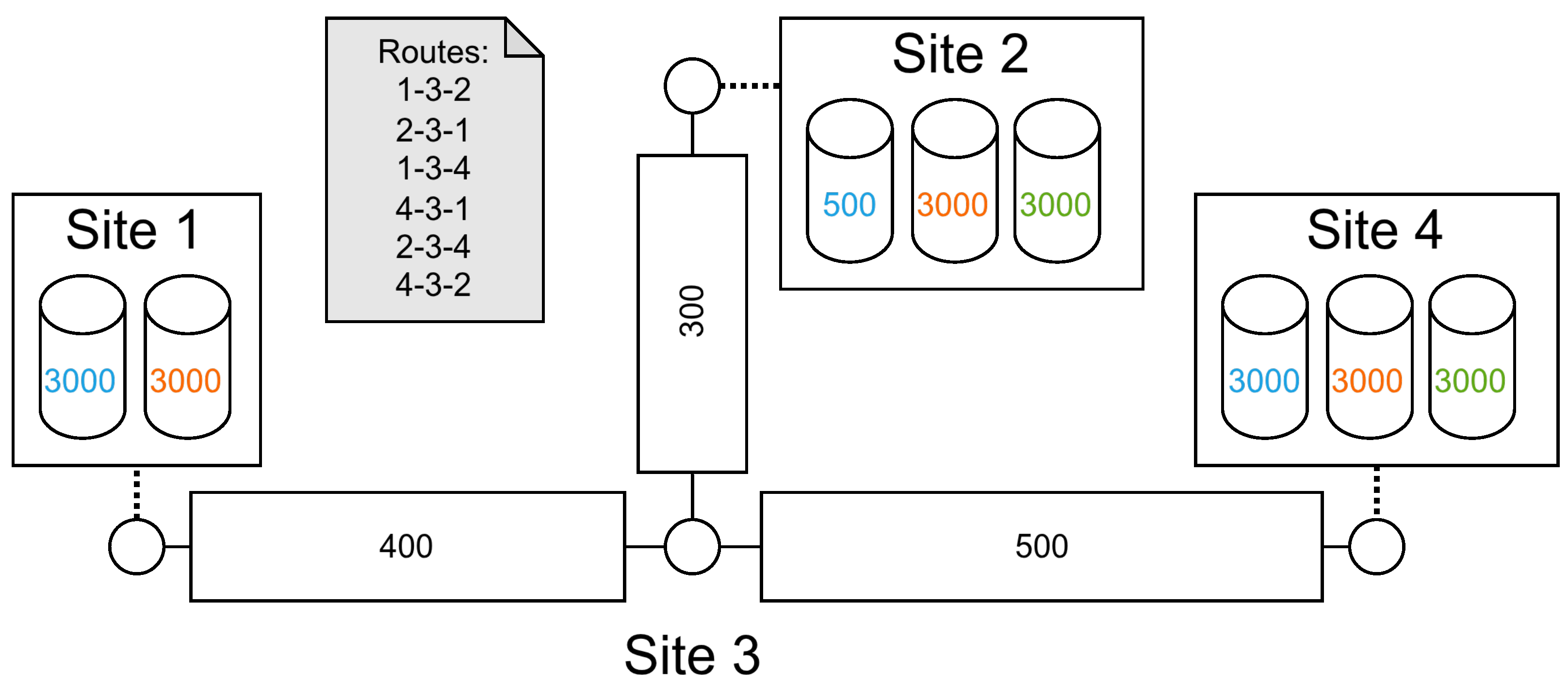
• Petroleum products managed in the network.
• Sites that contain an aggregate maximum tank capacity for each product. The minimum tank capacity is assumed to be zero. Sites are the nodes of the pipeline network.
• Pipe segments, or simply called pipes, which have a fixed volume and connect two distinct sites.
• Routes, which are paths connecting a source and a target site, consisting of adjacent pipes. A pumping operation can be performed over a route.
• Flow rates of considered pumping operations, inflows and outflows.

Further important details regarding the infrastructure definition are the following.

• The roles of sites are not determined. A site can be a production site, an intermediate node, a delivery station, or any combination of these. These are rather decided in the snapshot part, in the form of the planned inflows and outflows.
• A pumping operation is allowed not only via a single pipe, but a path of interconnected pipes from a source and a remote target site. A route may contain intermediate sites which do not participate in the pumping operation. However, not all such paths in the network are valid for pumping; therefore, allowed routes are explicitly listed in the problem description.
• A site may participate in multiple simultaneous pumping operations, via different routes. However, a pipe may participate in a single pumping operation at any given time.

Note that a real-world pipeline management application may consider further data. For example, opening hours for delivery sites, pipe and tank maintenance hours, or minimum capacities. These are omitted for simplicity in the current formulation.

An infrastructure for an example problem is shown in Figure 2.

In the example problem, the pipeline network transfers three petroleum products, shown by colors blue, orange, and green and consists of four sites and three pipes of volumes 400 ${\mathrm{m}}^3$, 300 ${\mathrm{m}}^3$, and 500 ${\mathrm{m}}^3$. Sites have a default capacity of 3000 ${\mathrm{m}}^3$ per product, with the following exceptions.

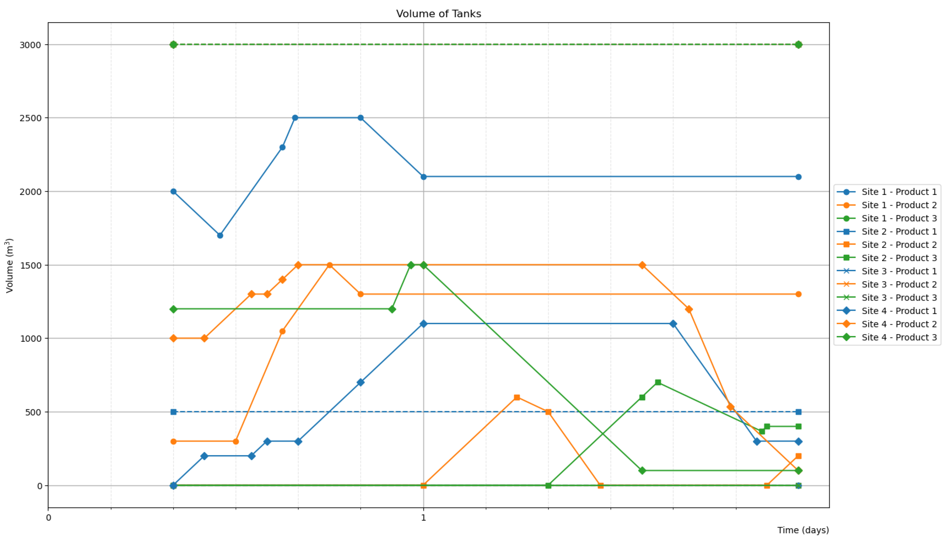
• Site 1 cannot store product 3 (green).
• Site 2 can store a limited 500 ${\mathrm{m}}^3$ of product 1 (blue).
• Site 3 has no tanks, and it cannot store any products. It is an intermediate node.

There are six routes for pumping: from any of sites 1, 2, and 4 to any other. Each route has two pipes. It can be observed that a pumping can be performed on at most one of the six routes at once, since any two routes are non-disjoint.

Note that the pipeline system permits reversed flow in any pipes. Therefore, despite being a tree of only four nodes, this simple network layout is already outside the scope of most literature models, which are designed for straight and sometimes tree-like networks. This example problem is topologically equivalent to a mesh-like network.

3.1.2. Snapshot Data

The second part of a scheduling problem instance is a snapshot of the system. In contrast to the infrastructure, a snapshot of a network contains data that corresponds to a time point during the time horizon and is supposed to change over time. The snapshot provided as part of the problem description corresponds to the initial time point of $t=0$, which is the start of the time horizon. A snapshot contains the following data.

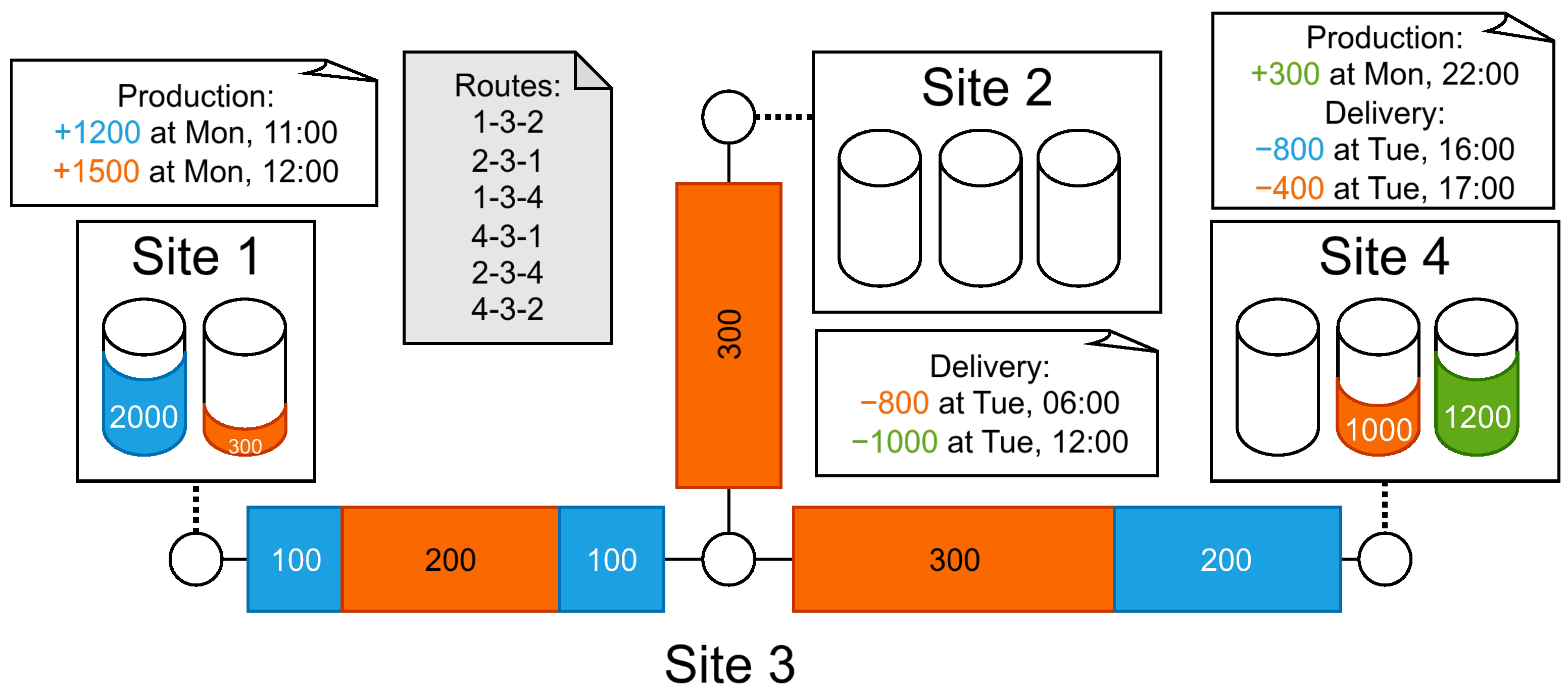
• Current tank inventory for all products in all sites.
• Current pipe contents, which are a list of plugs of different products.
• Given future inflows and outflows that are expected to happen. Each inflow or outflow is described by a start time, a site, a product, and an amount.

Important details regarding the snapshot definition are the following.

• Aggregate tanks are assumed. Therefore, each site is supposed to contain a single tank for each product. Operations relying on dedicated tanks (e.g., blending operations) are not directly modeled.
• Tank inventories should be between the minimum and maximum capacities, which are zero and the capacity given by the infrastructure, respectively.
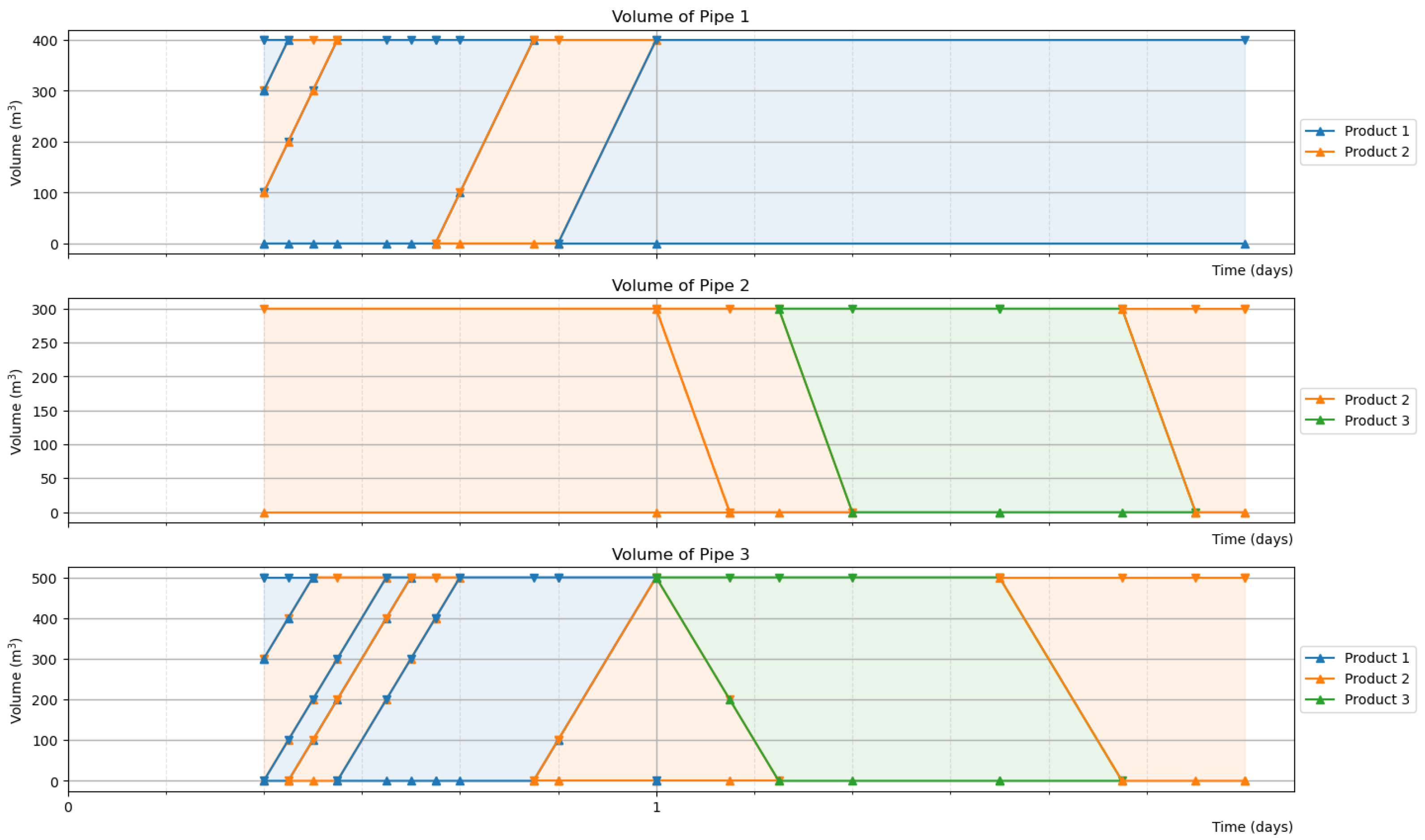
• Plugs in a pipe must always sum up to the constant volume of the pipe.
• Other than product type, no additional information is stored per plug. In particular, plugs are not assigned to specific batches or specific target sites, but simply end up being pushed out somewhere, influenced by subsequent pumping operations.
• Inflows and outflows represent material flows coming inside and going outside the pipeline network. Such flows only happen at site tanks, never from the pipes directly. These can model receiving of products from outside, production, blending operations, delivery, and other operations.
• Inflows and outflows are not instantaneous but continuous. For the sake of simplicity, the flow rates for inflows and outflows each are assumed to be constants given as infrastructure data.

An example snapshot for the starting point 08:00 Monday is shown in Figure 3.

In the example snapshot, the following volumes of the products exist in the system.

• For product 1 (blue), there is a stock of 2000 ${\mathrm{m}}^3$ at site 1, and 400 ${\mathrm{m}}^3$ is already present in two pipes, as three distinct plugs of sizes 100 ${\mathrm{m}}^3$, 100 ${\mathrm{m}}^3$, and 200 ${\mathrm{m}}^3$.
• For product 2 (orange), there is a stock of 1000 ${\mathrm{m}}^3$ at site 4, and 800 ${\mathrm{m}}^3$ in three different pipes, in plugs of size 200 ${\mathrm{m}}^3$, 300 ${\mathrm{m}}^3$, and 300 ${\mathrm{m}}^3$.
• For product 3 (green), there is a stock of 1200 ${\mathrm{m}}^3$ at site 4.

The future production and delivery plans indicate the roles of the sites. These are represented by outflows, listed in

Table 1. Inflows and outflows for the example problem.

Start Time	Site	Product	Amount	In/Out
Day 1, 11:00	Site 1	Product 1 (blue)	1200${\mathrm{m}}^3$	Inflow
Day 1, 12:00	Site 1	Product 2 (orange)	1500${\mathrm{m}}^3$	Inflow
Day 2, 06:00	Site 2	Product 2 (orange)	800${\mathrm{m}}^3$	Outflow
Day 2, 12:00	Site 2	Product 3 (green)	1000${\mathrm{m}}^3$	Outflow
Day 1, 22:00	Site 4	Product 3 (green)	300${\mathrm{m}}^3$	Inflow
Day 2, 16:00	Site 4	Product 1 (blue)	800${\mathrm{m}}^3$	Outflow
Day 2, 17:00	Site 4	Product 2 (orange)	400${\mathrm{m}}^3$	Outflow

.

3.1.3. Schedule Description

A schedule is a solution of the multiproduct pipeline scheduling problem. A schedule is a set of pumping operations to perform during the time horizon given the following:

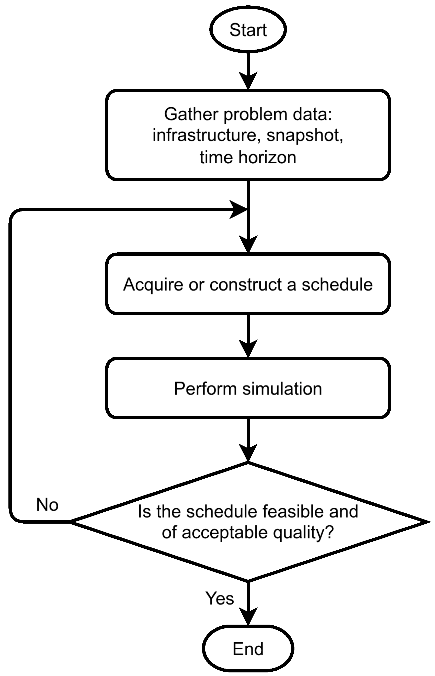
• The infrastructure of the pipeline network,
• A snapshot of the given infrastructure,
• A time horizon of length H, which starts at the time point the snapshot corresponds to.

Each pumping operation is characterized by the following attributes:

• Starting time (within the time horizon).
• Ending time (after the starting time, within the time horizon).
• The route on which the pumping operation is performed.
• The product which is being pumped.

Important notes are the following.

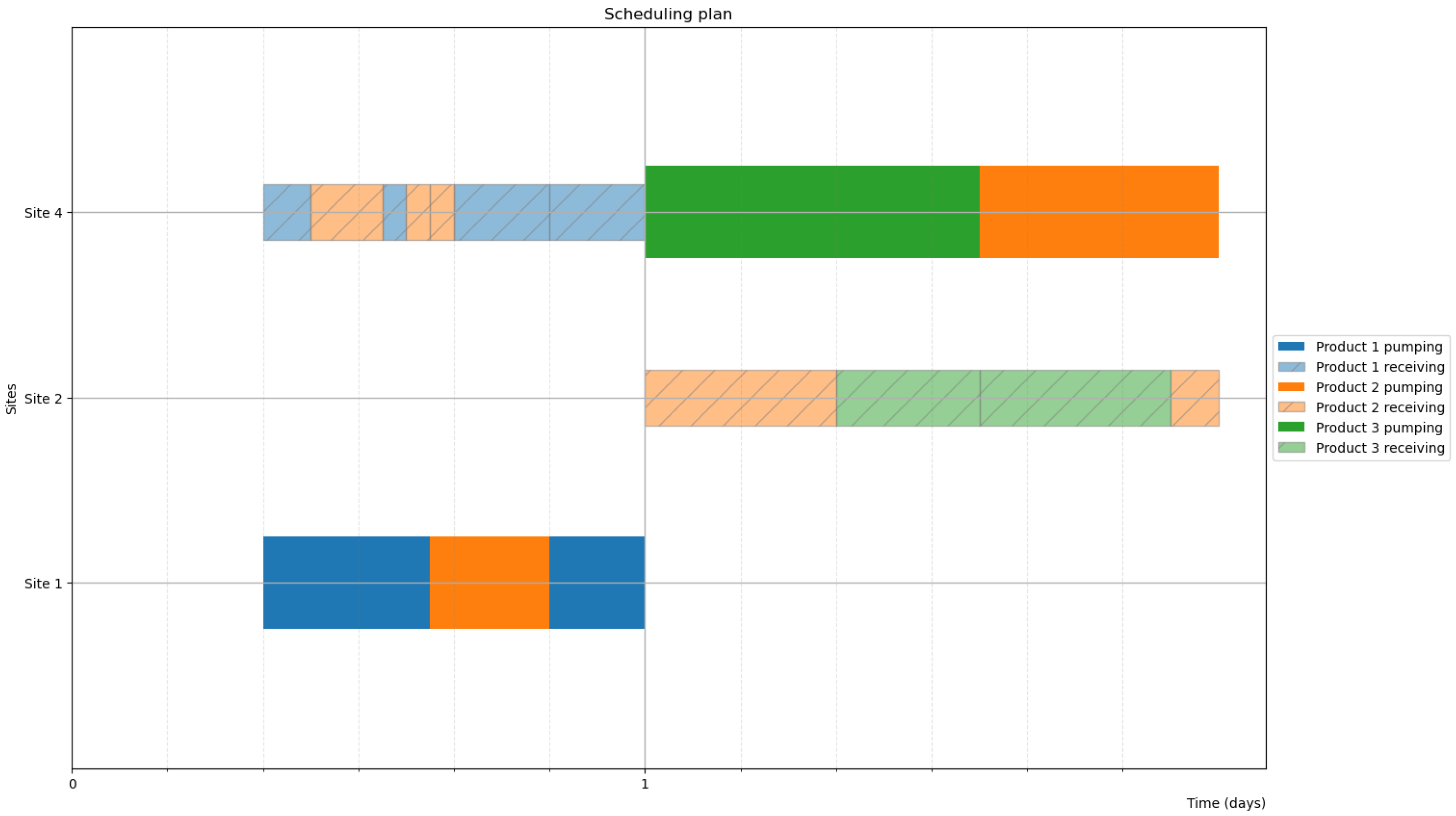
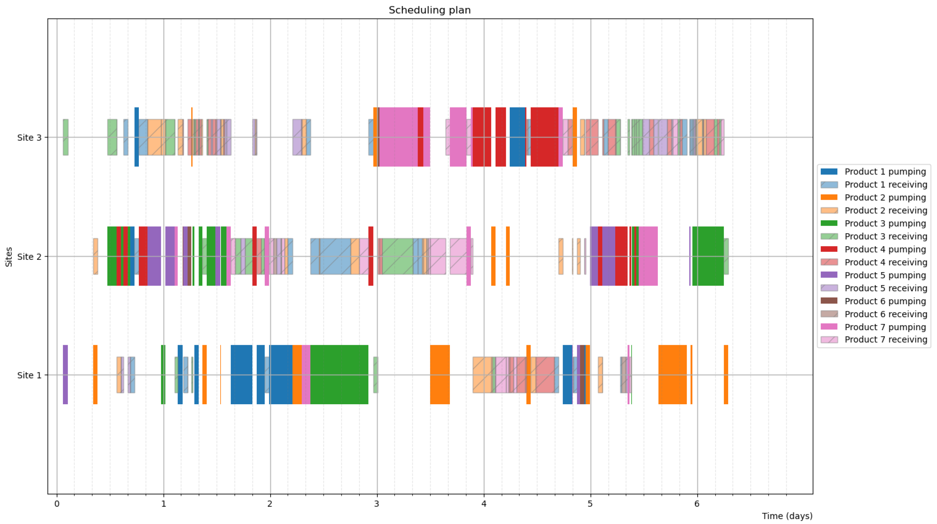
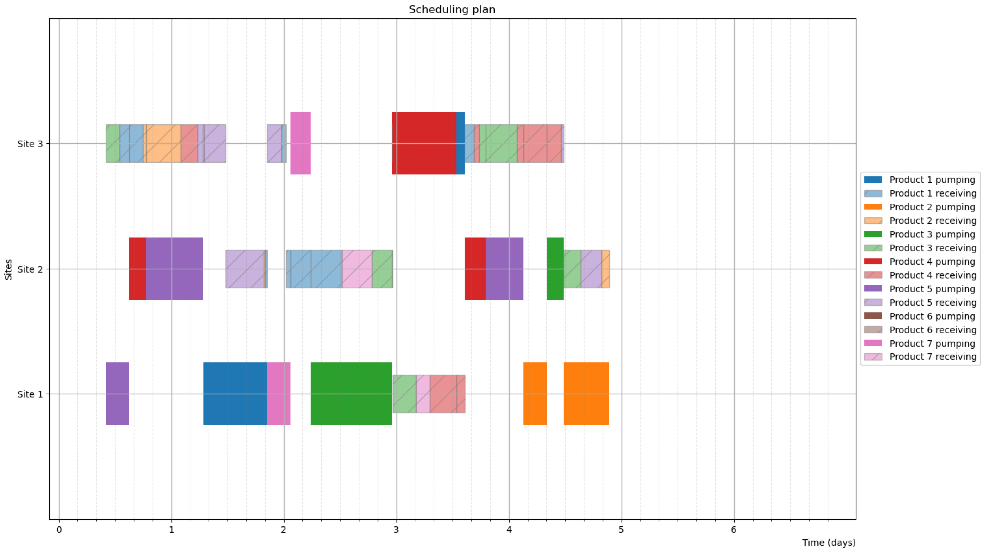
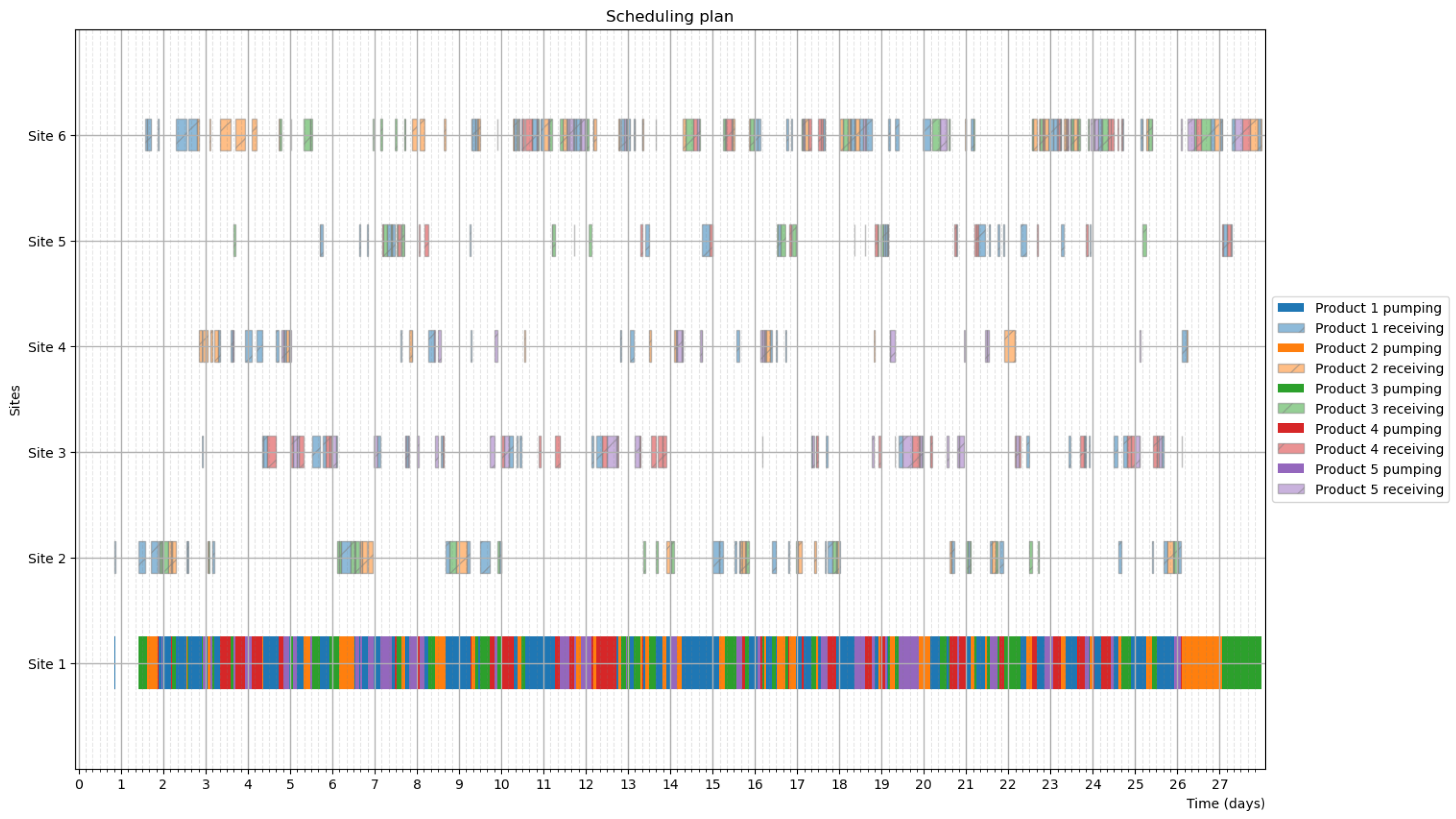
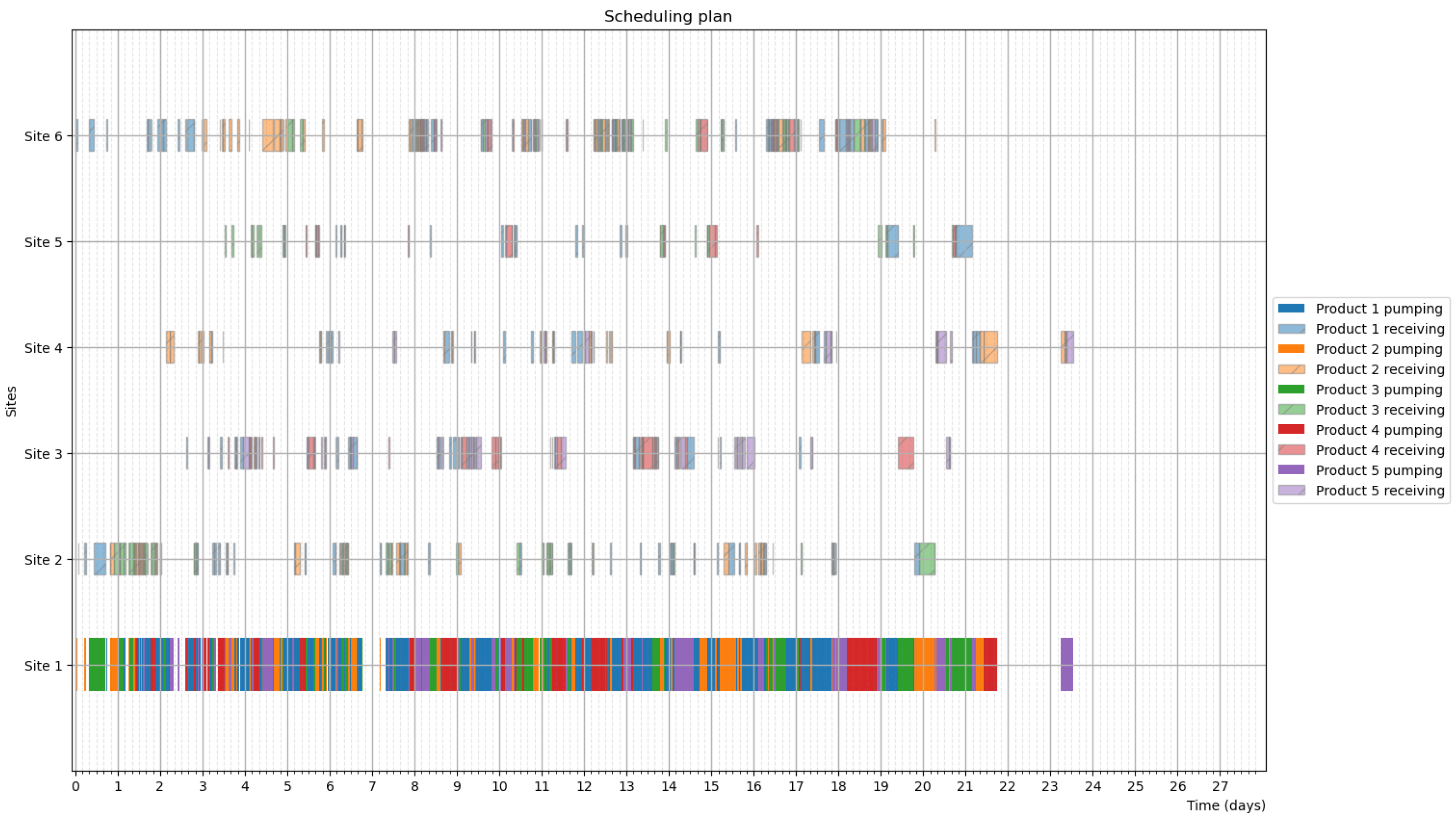
• A schedule determines what happens in the pipeline network in full detail.
• Pumping volumes are indirectly determined by the pumping start and end times and the flow rates. Expressing pumping operations by time rather than volume makes it easier to design a contradiction-free schedule.
• Source and target sites, as well as the involved pipes are determined by the route chosen.
• The product which is pushed out at the target site and uploaded to a tank is indirectly determined by the actual pipe contents at the last pipe of the route. Therefore, the product pushed out at the target site may change during the same pumping operation, but the product pumped at the source site always remains the same.

Given this framework, a set of pumping operations constitutes a feasible schedule unless either of the following conditions holds:

• Condition 1: Two pumping operations overlap for which the routes have a common pipe.
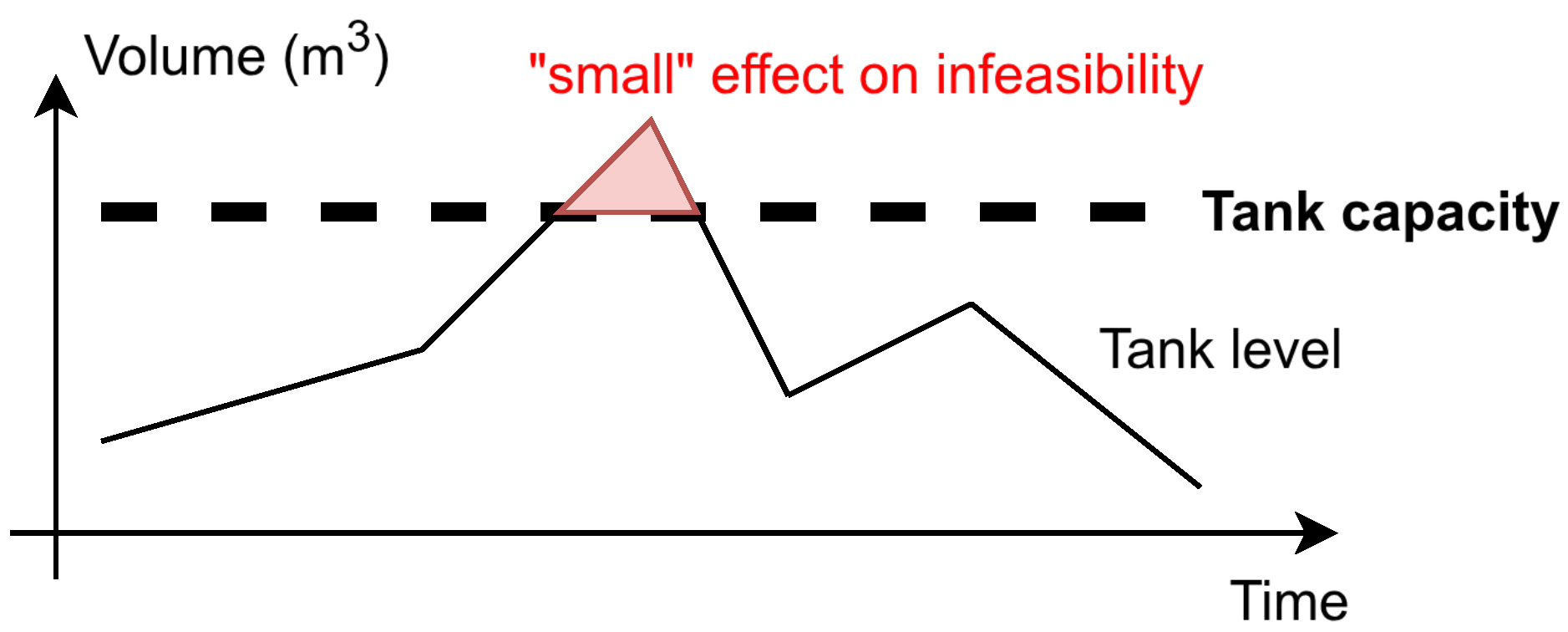
• Condition 2: The stored amount of a product at a site goes below zero or above tank capacity.

If any two routes have a pipe in common, then Condition 1 is simplified into all pumping operations not overlapping. This is simple to check or ensure during schedule generation. Therefore, the key reason for infeasibility is Condition 2, which means that tank levels should be maintained within the minimum and maximum levels at all sites for all products within the time horizon.

Note that the simulation itself is never interrupted. All flow changes, either from in/outflows given as input, or pumping operations given as scheduling decisions, are performed, even beyond minimum or maximum tank capacities.

A schedule for the example problem is given in

Table 2. Schedule for the example problem, consisting of pumping operations.

Start Time	End Time	Route	Product
Day 1, 08:00	Day 1, 15:00	1-3-4	1 (blue)
Day 1, 15:00	Day 1, 20:00	1-3-4	2 (orange)
Day 1, 20:00	Day 2, 00:00	1-3-4	1 (blue)
Day 2, 00:00	Day 2, 14:00	4-3-2	3 (green)
Day 2, 14:00	Day 2, 00:00	4-3-2	2 (orange)

. The time horizon is 40 $\mathrm{h}$, starts at 08:00 Monday (day 1), and ends 40 h later at 00:00 Wednesday (day 3). Although this schedule contains no idle periods between pumping operations, such pauses are not required by the model.

The schedule is also depicted as a Gantt chart in Figure 4. The x-axis represents the time horizon, and the y-axis represents the sites of the pipeline network. The solid, thick bars represent that a site is a pumping source. The pale, thinner bars represent that a site is receiving material from a pumping operation, originated from another site. This Gantt chart format can depict all information regarding a schedule if there are no overlapping pumping operations and no ambiguous routes between a pair of sites. Solid bars are always paired with pale bars.

Note that the received products are not part of the schedule but are determined by the schedule. Getting these data and deciding whether a schedule is feasible is not trivial. This necessitates the use of a simulator.

3.1.4. Expected Simulator Output

The goal of a simulator is to evaluate a schedule, answering basic questions about it and providing detailed data for further analysis. Given an infrastructure, the starting snapshot, the time horizon, and a schedule, the simulator is expected to calculate the following over the whole time horizon. Each component and the motivation behind it is explained.

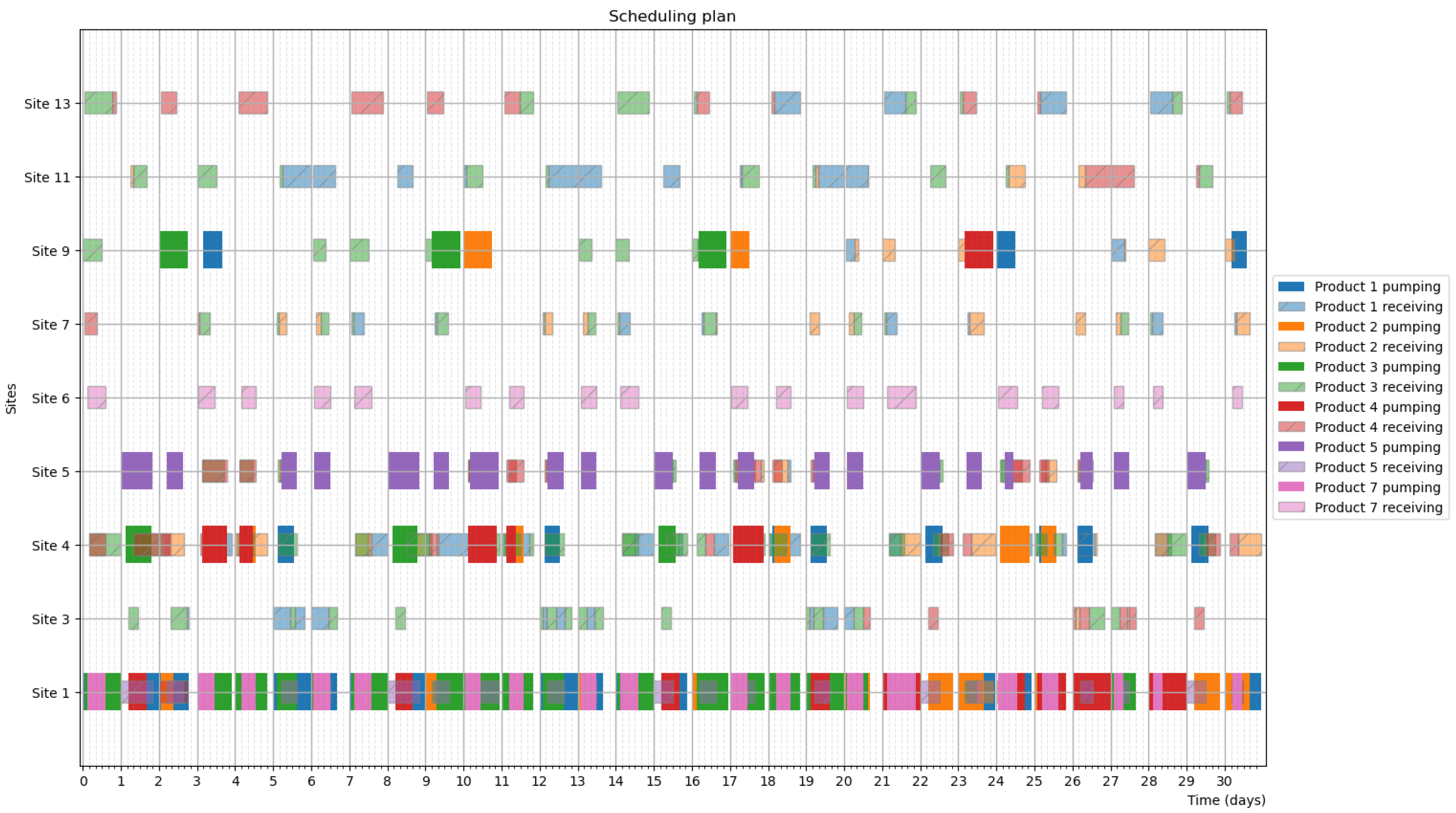
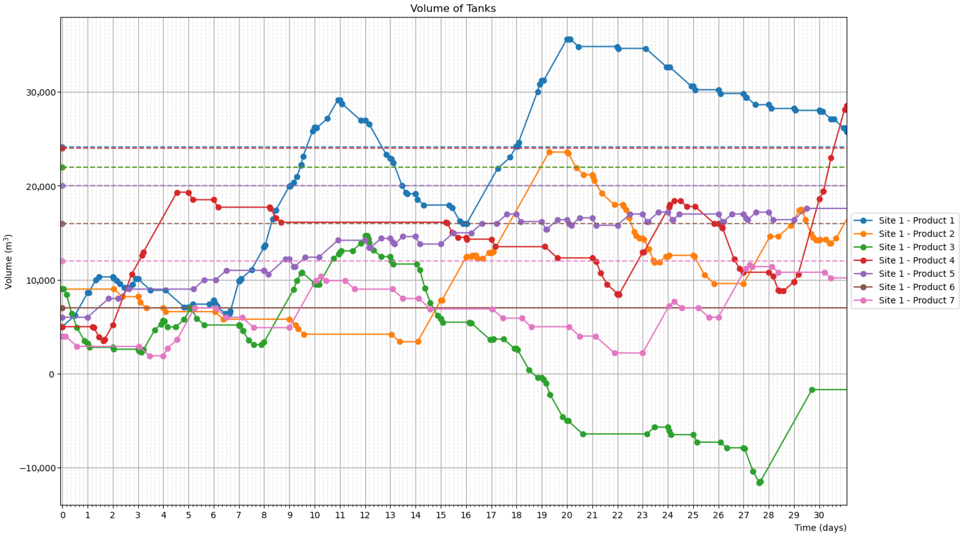
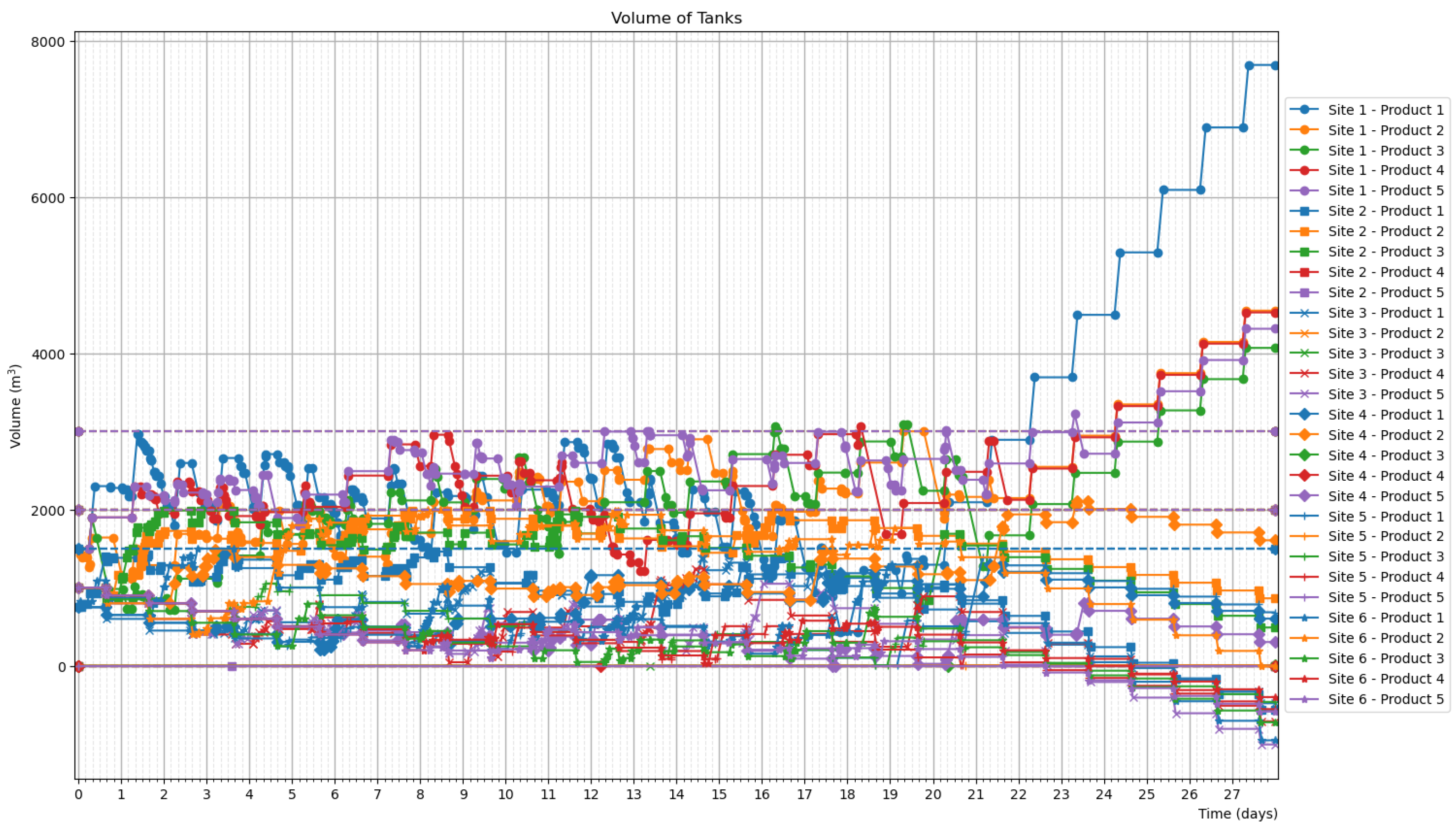
• Detailed tank level profiles for each product at each site.
• Detailed pipe contents for each pipe segment.
• Tracking of interfaces.
• Quality measures.

Tank level profiles are crucial for determining whether a schedule is feasible. Tank levels below zero or above the capacity are the only non-trivial way a schedule can be infeasible. The level of each product at each site can be given as a piecewise linear function. Figure 5 shows the tank level profiles obtained for the example scheduling. Note that some flow rate changes are not caused by pumping, but the planned inflows and outflows. The example schedule is feasible.

Detailed pipe contents could be useful for further analysis. These are currently used solely for visualization, a common practice in related studies. Figure 6 shows the pipe contents for the example schedule. The x-axis represents the time horizon, and the y-axis represents the volume of plugs inside a pipe. The diagram clearly shows how the interfaces between different products move and the flow reversal that took place at Day 2, 00:00, in pipe 3 (between sites 3 and 4). In both figures, the markers represent event points where the slopes of the piecewise linear functions may change.

The tracking of interfaces is important for calculating interface-related costs and the expected extent of product contamination. Although the exact rules for interfaces are not determined yet, the simulator was required to track each interface in the pipeline network.

Quality measures are statistics to be possibly used in objective functions, which are the easiest to calculate during the simulation procedure itself. The following quality measures were explicitly chosen.

• Number of interfaces (already present or created).
• Total persistence duration of interfaces.
• Number of flow reversals.
• Number of pumping operations.

The number of interfaces and their total persistence, which is the sum of durations the interfaces were present, affects how much contaminated product is expected. These are for demonstration; due to interface tracking, other measures could easily be calculated. Flow reversals and pumping operations are directly associated with turning pumps on and off, which is recognized as a significant cost factor by many works in the literature.

The problem definition can be concluded as follows: given a pipeline infrastructure, a current snapshot, and a time horizon, find a schedule which is feasible within the time horizon and has the best possible quality measures.

3.2. Simulation Algorithm

For the multiproduct scheduling problem formulation, a simulation algorithm is proposed. This accepts an infrastructure, a snapshot, a time horizon, and a schedule, and calculates the desired results.

3.2.1. Event System

The simulation algorithm is a Discrete-Event Simulation approach. Although the flow of products inside pipelines is continuous, there is a limited set of event points resulting in structural change of flows. Between two consecutive events, all quantities in the system can be predicted and calculated. Therefore, the simulation of a finite set of event points of the continuous process reduces to a discrete problem.

The algorithm proceeds by increasing the current time from the start to the end of the time horizon, while a set of future events is maintained. Only the earliest of the future events is processed at once. Scheduling time points are stored at the granularity of 1 $\min$. The simulation algorithm is shown as pseudocode in Algorithm 1. The possible events are summarized in

Table 3. Events in the simulation algorithm, their summarized effects, and upcoming events.

Event Type	Tank FR Increase	Tank FR Decrease	Plug FR Change	Interface Change	Next Event(s) Possibly Generated
Inflow start	Yes	No	No	No	Inflow end, start
Inflow end	No	Yes	No	No	Inflow start
Outflow start	No	Yes	No	No	Outflow end, start
Outflow end	Yes	No	No	No	Outflow start
Pumping start	Yes	Yes	Usually	Possible	Plug event, pumping end
Plug event	Possible	Possible	Yes	Yes	Plug event, pumping end
Pumping end	Yes	Yes	Usually	Possible	Pumping start

.

Algorithm 1 Main event loop of the simulation algorithm.

$time\leftarrow 0$ (time horizon start) $Events\leftarrow$ set of initially generated events while  $time\le H\wedge Events\ne \varnothing$  do       Choose $e\in Events$ so that StartTime(e) is minimal       $Events\leftarrow Events\setminus \left\{e\right\}$       $time\leftarrow$ StartTime(e)       Process(e)       $Events\leftarrow Events\cup$ NextEvents(e) end while

In the context of the simulation algorithm, flow rate (FR) is the volume of a tank or plug expressed as a function of time, assuming that no further events will ever occur. Events can induce flow rate changes in tanks and/or plugs. Also, pumping and plug events may change the plugs and interfaces.

An important optimization used in the algorithm is that at any time point during the simulation, only a small subset of future events are kept in program memory. For example,

• Inflow (and outflow) start events are known a priori, so only the next one is considered.
• An inflow (and outflow) end is only considered after its corresponding start.
• Plug events describe structural changes during a pumping operation, and at each such event, only the next one can be and needs to be calculated.

New events need to be generated after another event was processed. Therefore, Table 3 also shows what other upcoming events are typically generated after a given event is processed.

Note that this event system does not require the pipeline network to be evaluated at fixed time slots, e.g., every 1 h or 1 min, as some previous approaches [4]. Moreover, at each event, only a limited part of the pipeline network is affected. This results in a significant increase in computational speed and was the most important motivation for the current work.

3.2.2. Pumping Events

Each pumping operation affects the following components of the pipeline network.

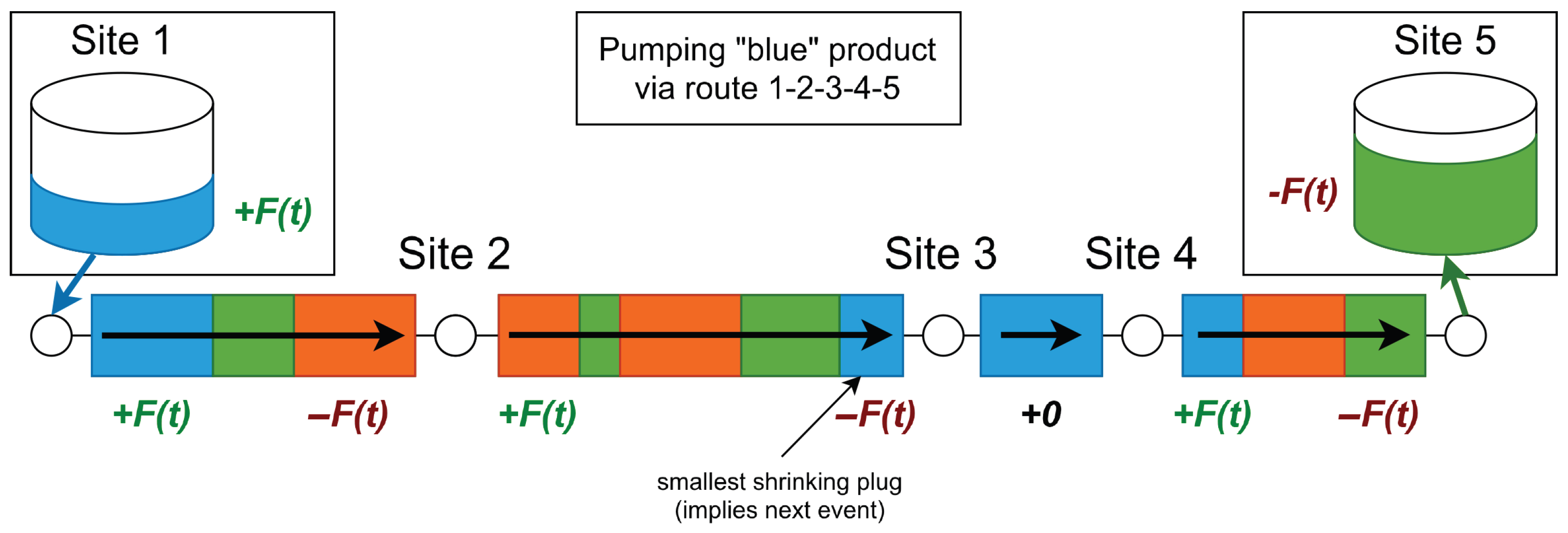
• The tank of the source product at the source site that is currently being pumped.
• The tank of the product currently being pushed out at the target site.
• The plugs in the pipes on the route of the pumping operation.
• Interfaces between plugs.

Suppose that pumping is performed at a pumping flow rate function $F\left(t\right)$. This means that after t time has elapsed, a total volume of $F\left(t\right)$ is injected at the source site. Then, the two tanks at the source and target sites and all first and last plugs are subject to a volume change of either exactly $+F\left(t\right)$ or $-F\left(t\right)$. Volume from each shrinking plug at the end of the pipe is transferred to another, growing plug in the next pipe or the target tank. This is the consequence of the liquids in pipes being incompressible. If a pipe contains a single plug, then the $+F\left(t\right)$ and $-F\left(t\right)$ effects cancel each other out, so the flow rate for that plug is zero.

The volume changes are shown in Figure 7. Note that the plugs can only be altered by the current pumping operation, but tanks can be subject to other flow rate effects (e.g., inflows, outflows, and other pumping operations).

Between pumping start and end events, it is possible that the end of a plug reaches the end of a pipe, which generates a plug event.

The next plug event is always determined by the smallest shrinking plug. If the size of the last plug of pipe p is $V_p^{last}$ at the current time of the simulation, then the pipe p for which the next plug event will occur, and the time t elapsed until that event are determined by Equation (1). This describes that, among all pipes in the route, the volume of the smallest shrinking plug determines the next event.

$$F\left(t\right)=\underset{p\in Route}{min}{V}_p^{last}$$

(1)

The plug event, also illustrated in Figure 8, causes the following effects.

• The source tank and all shrinking plugs are decreased by $F\left(t\right)=V_p^{last}$.
• The target tank and all growing plugs are increased by $F\left(t\right)=V_p^{last}$.
• Plugs with a remaining volume of zero are removed.
• If p was the last pipe of the route, the product that is pushed out might change, so the target tank flow rates are updated. Otherwise, a new growing plug is inserted to the pipe after p, with a volume of zero.

3.2.3. Interface Management

The simulator monitors each interface during its lifetime. The following rules apply.

• Interfaces exist initially between plugs of different products.
• New interfaces are created only at pumping start events at the beginning of a pipe in the route (see Figure 9).
• Interfaces are only removed when arriving at a target site.
• Interfaces may move from one pipe to another during a plug event when a corresponding plug shrinks to zero.

Note that there are edge cases for interface management. First, an interface is not only created at pumping sites, but intermediate nodes as well, if a pumping operation splits a product batch that did not fully leave an intermediate node. It is also possible that an interface is stopped exactly at an intermediate node, in which case it may move away with a next pumping operation.

The algorithm can possibly create very small plugs when an interface stops close but not exactly at an intermediate site. This may happen when a pumping is close to but does not have the desired duration. Such situations may result in additional interfaces. To avoid such small plugs, a threshold $V^{plug,min}$ is used. When a pumping end event is processed $F\left(t\right)<V^{plug,min}$ volume after the last plug event of the same pumping operation, then that final volume after the last plug event is simply not pumped. In effect, the pumping ends earlier, at its last plug event.

3.3. Optimization by Local Search-Based Algorithms

The aim of developing an optimization algorithm was to demonstrate the efficiency of the simulator, and to provide a best effort for automatic schedule construction.

The algorithm is based on local search. An initial schedule is generated, then small perturbations are applied. A perturbation is a small change to an existing schedule, resulting in a similar but slightly different schedule for the same problem instance. Each schedule is evaluated by the simulator. If a new schedule with a better fitness is found, the current schedule is replaced.

Three variants for optimization were implemented, tested, and are presented here. The pseudocodes for the three variants can be found in the Appendix A.

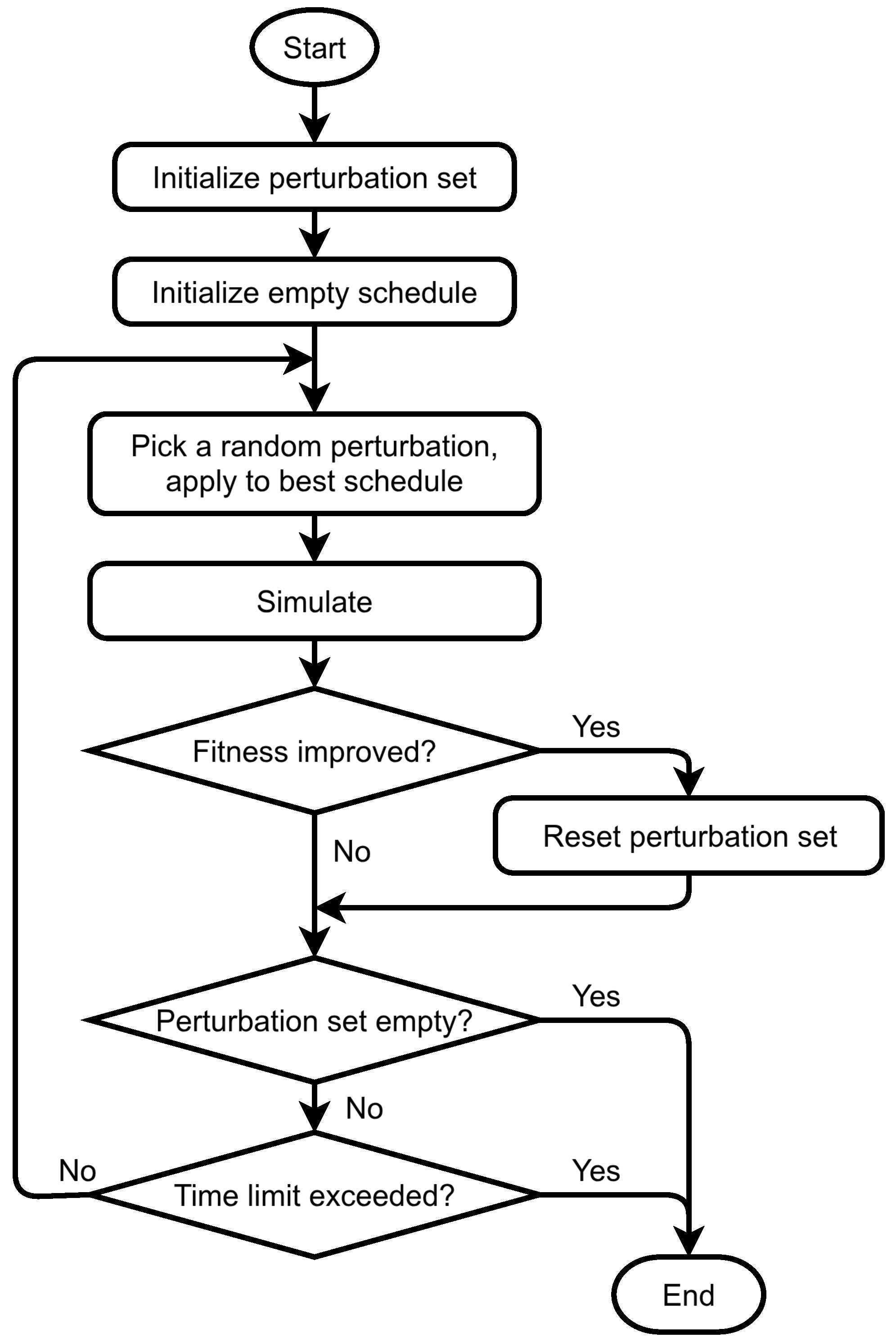
• Exhaustive variant.
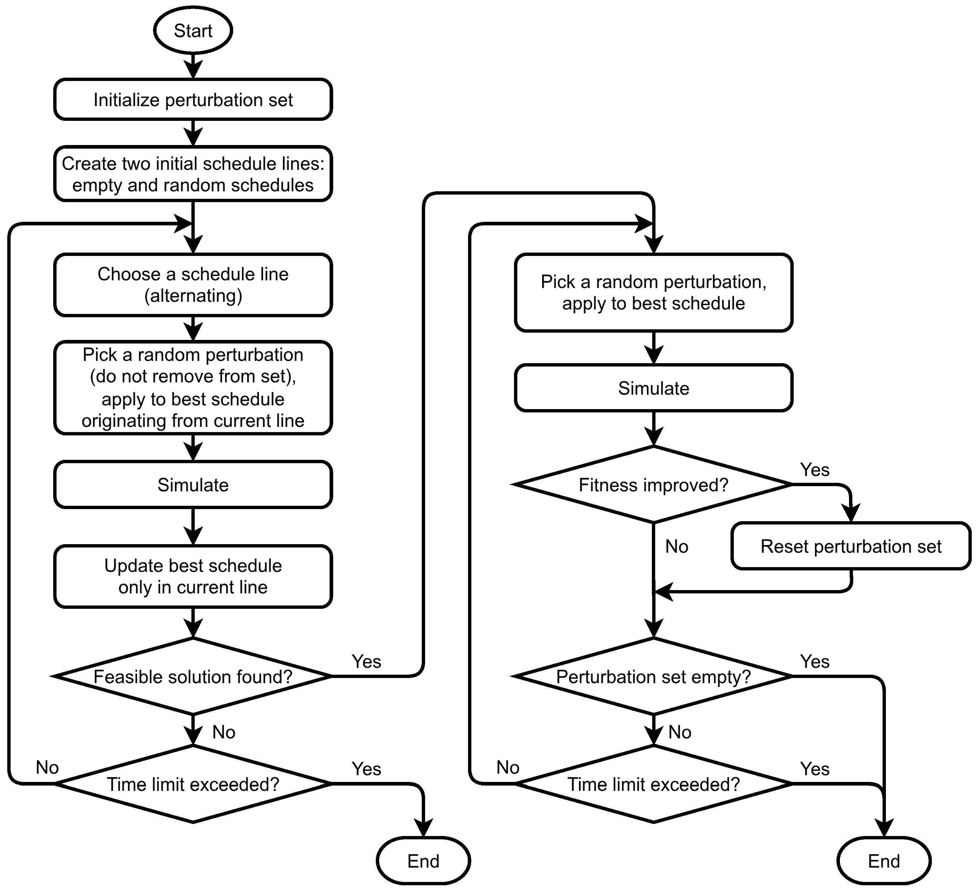
• Look-ahead variant.
• Simulated annealing variant.

Although the simulation algorithm would allow parallel pumping operations, the optimization algorithms presented here only use mutually exclusive pumping times, which are easier to manage and to perturb.

3.3.1. Two-Stage Fitness Function

A schedule may be infeasible if tank levels go below zero or above the capacity. Therefore, a two-stage fitness function is used. The first stage is an objective which expresses the degree of infeasibility of a schedule. The second stage is another objective which expresses the quality of a schedule. As will be shown, these are contradicting goals. Therefore, when comparing schedules, the first-stage objective is considered first. If these are equal (for example, when both schedules are feasible), then the second-stage objectives are compared.

As the first-stage objective, the following were considered during development.

• Global earliest tank violation time:

  $$t^{violation,first}=min\left\{\underset{h\in Tanks}{min}{T}_h^{+},\underset{h\in Tanks}{min}{T}_h^{-}\right\}$$

  (2)
• Time-adjusted sum of first tank violation times:

  $$t^{sum}=\sum _{h\in Tanks}\left(e^{H-\lambda T_h^{+}}+e^{H-\lambda T_h^{-}}\right)$$

  (3)
• Time-adjusted sum of violation volumes:

  $$w^{sum}=\sum _{h\in Tanks}{\mathit{\int }}_0^H{e}^{H-\lambda t}\left(max\left\{V_h\left(t\right)-V_h^{max},0\right\}+max\left\{V_h^{min}-V_h\left(t\right),0\right\}\right)dt$$

  (4)

In these formulas, $T_h^{+}$ and $T_h^{-}$ denote the first violation times, when tank h is overfilled above maximum capacity or depleted below zero. If there is no such violation, then the first violation time is $+\infty$. $\lambda ={\displaystyle \frac{log2}{1\mathrm{day}}}$ was used. Informally, this means that a violation is twice as bad for each day earlier it happens. $V_h\left(t\right)$ is the level of tank h at time point t. $V_h^{max}$ is the tank maximum capacity, and $V_h^{min}=0$ is the tank minimum capacity, always zero.

Some discussion about these first-stage objectives is given below. The problem formulation does not allow sudden jumps in tank or pipe levels, as all flows are continuous. This makes $t^{violation,first}$ and $t^{sum}$ respond better to perturbations that slightly alter an infeasible tank volume into the good direction, since such an alteration also affects the first violation time for that tank. $w^{sum}$ was introduced to allow improvements to tank profiles beyond and possibly not affecting the first violation times. Note that $w^{sum}$ also has a disadvantage: if a violation is very short and small, its overall effect can be close to zero, while technically making the whole schedule infeasible (see Figure 10).

The second-stage objective expresses the quality of a schedule. It is defined as a simple aggregate $q^{sum}$, following the measures introduced in the problem formulation, see Equation (5). Here, ${\varphi }^{count}$ is the number of interfaces existing during the simulation, ${\varphi }^{time,alive}$ is the total duration of interfaces existing in minutes, $b^{count}$ is the number of flow reversals or backtransports per pipe, and $p^{count}$ is the number of pumping operations.

$$q^{sum}=50·{\varphi }^{count}+0.1·{\varphi }^{time,alive}+20·b^{count}+10·p^{count}$$

(5)

3.3.2. Exhaustive Optimizer

The exhaustive variant relies on a set of predefined perturbations. Starting from the empty schedule, a random perturbation is applied and accepted only if the fitness is improved. This continues until the time limit is exceeded, or the algorithm exhaustively runs out of perturbations without improving fitness since the last update. The algorithm is illustrated in Figure 11 and with pseudocode in Appendix A as Algorithm A1.

The perturbations are defined using the following interval generation scheme. Suppose that the time slot length is L. Then, a set of intervals $I_L$ can be generated, as in Equation (6). This allows intervals of variable lengths but with a total cardinality of $O(HlogH)$, which is a compromise between completeness and computational costs.

$$I_L=\left\{\left(kL,(k+2^t)L\right):k,t\in {\mathbb{N}}_0,(k+2^t)L\le H\right\}$$

(6)

The set of perturbations is constructed as follows.

• For $L=60\min$, define perturbations for $(x,y)\in I_L$ and for all routes and products, as adding a pumping operation at $(x,y)$, by insertion or replacement (for two perturbations in total). Insertion differs from replacement in that the overwritten pumping operations are shifted forward.
• For $L=15\min$, define perturbations for $(x,y)\in I_L$ as clearing the schedule between $(x,y)$, shifting down to x, grouping the same type of pumping operations together within $(x,y)$, reversing the schedule within $(x,y)$, and moving a pumping operation at x from y, or vice versa (for six perturbations in total).
• For $L=5\min$, for time points $x\in \left\{kL:k\in {\mathbb{N}}_0,kL\le H\right\}$, define perturbations as clearing, filling, or shifting one pumping operation below and above x (for six perturbations in total).

Note that the first group of perturbations, which involve pumping insertions and replacements, are aimed at obtaining feasibility of the schedules. The other two groups are aimed at fine-tuning the schedule quality by decreasing its overall complexity.

The exact definition of each perturbation can be found in the Supplementary Material.

3.3.3. Look-Ahead Optimizer

The look-ahead variant is similar to the exhaustive variant, but it has a slightly different perturbation mechanism. The algorithm is illustrated in Figure 12 and pseudocode in the Appendix B as Algorithm A2.

The main differences of the look-ahead variant are the following.

• Instead of the empty schedule, the look-ahead proceeds on two separate, alternately improved lines using two starting schedules: one line starting with an empty schedule and one line starting with a schedule randomly filled with pumping operations of length $L=60\min$. These are alternatively perturbed until the first feasible solution is found.
• Pumping operations are not from a set of perturbations to be exhausted. There is an $85\%$ chance of adding a pumping operation. After the first feasible schedule is found, this chance is set to $15\%$.
• When adding a pumping operation, a random starting time is always chosen before the first tank violation. Then, there is a $25\%$ chance to set the pumping duration to a fixed $L=60\min$, or a $75\%$ chance to set it by looking ahead. The look-ahead setting performs a new simulation, assuming the added pumping ends at the end of the time horizon. Then, the first tank violation denotes the chosen end time of the added pumping operation. This algorithm uses two simulations in total for performing one perturbation. The rationale behind this look-ahead mechanism is not to cause infeasible situations while performing as much pumping at once as possible with a single perturbation.

3.3.4. Simulated Annealing Optimizer

The simulated annealing variant works exactly like the look-ahead variant, but acceptance of a perturbation is possible, even if the fitness is worse.

• The starting value of temperature T is the number of possible route–product pairs for pumping.
• An exponential cooling and acceptance regime is applied [35]. The acceptance probability p is given by Equation (7).

  $$p=min\left\{e^{{\displaystyle \frac{ob{j}^{best}-ob{j}^{next}}{T}}},1\right\}$$

  (7)
  The objectives before and after perturbation are $ob{j}^{best}$ and $ob{j}^{next}$. Depending on whether a feasible schedule was already found, either the first stage or second-stage objective is used.
• Each time acceptance is considered, and T is multiplied by $1-{10}^{-4}$.
• When the first feasible schedule is found, T is reset. Afterwards, an infeasible schedule is never accepted.

The pseudocode of the simulated annealing variant can be found in the Appendix B, as Algorithm A3.

3.4. Possible Extensions

There are further problem components and constraints that are omitted from the current formulation, due to a limitation of the current implementation. Several such components are listed below, with possible resolutions.

• Aggregate tanks are currently assumed. Dedicated tanks could be handled by the simulator, provided that a logic is available for choosing an appropriate tank at the source and target sites. This is not expected to significantly affect the computational cost of a simulation. A policy for automatic choice of the tank by the simulator is a possibility and already used in practice. Alternatively, dedicated tanks can be coded as a scheduling decision, but that could introduce a new kind of infeasibility: when the product arriving at a target site does not match the target tank.
• Tank availability changes are rare but can be possibly planned. When a tank is down (for example, due to maintenance or opening hours), any pumping-related inventory change can be included in the first-stage fitness function as a penalty and handled in the same manner as for tank level violations.
• Forbidden product pairs for interface formation are currently not handled. However, since the simulation already tracks interfaces, large penalties can be introduced if specific products become in contact.
• The simulation algorithm can handle parallel pumping operations, but the optimization algorithms currently do not consider this possibility. Parallel pumping operations would require a more sophisticated perturbation mechanism, which permits multiple, non-conflicting routes to be chosen for pumping in overlapping time intervals. Note that the simulation model can already handle tank flow rate changes from different sources, as pumping operations, inflows, and outflows may already overlap.
• Arbitrary flow rates could also be used. The simulator currently assumes $F\left(t\right)=C^{pumping}·t$ as the pumping flow rate, where $C^{pumping}$ is a constant for the problem instance. Other flow rates could be implemented as follows.

  −

  If the flow rate is a time-independent constant, the algorithm can be used without change to the event loop. An example scenario is when the pumping flow rate depends on the route and pumped product only, as if $F\left(t\right)=C_{site,product}^{pumping}·t$.

  −

  If the flow rate depends on current pipe contents, then ${min}_{p\in Route}{V}_p^{last}$ can be calculated as normal. Since there are no further effects until the next plug event occurs besides the volume changes of $+F\left(t\right)$ and $-F\left(t\right)$, Equation (1) can be solved for t. An example scenario is when the pumping flow rate depends on some weighted average of pipe contents.

4. Computational Results

To demonstrate the effectiveness of the simulation algorithm, and the capabilities of the local search-based optimization algorithm variants, the algorithms were tested on a set of example multiproduct pipeline scheduling problems, using varying time horizons. Results and findings are provided in this section. The test series is available in the Supplementary Material as source code, in an easily reproducible way.

4.1. Scheduling Problems

The following problems were involved in the case study.

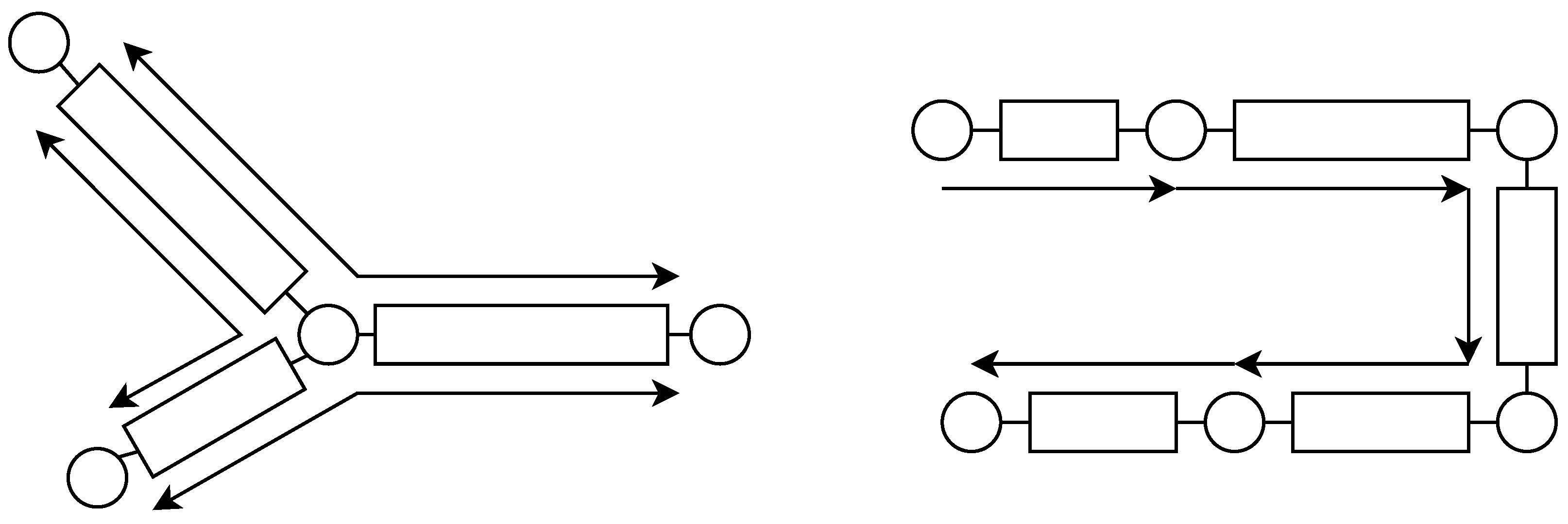
• Problem 1: y-junction network, with large tank capacities.
• Problem 2: y-junction network, with tight tank capacities.
• Problem 3: Straight network.
• Problem 4: Large-scale mesh-like network.

Problems 1–3 are synthetic problems for testing both the simulation and optimization algorithms. Figure 13 shows the topology of these problems. Problem 4 is a literature example, used to test the simulation algorithm only.

In Problems 1–2 with the y-junction network, the infrastructure contains seven different products; pipes with volumes 500 ${\mathrm{m}}^3$, 800 ${\mathrm{m}}^3$, and 300 ${\mathrm{m}}^3$; and six routes: from any non-central node to any other. The network shape and route set are the same as in the example problem the formulation was demonstrated on. There is a total of 1600 ${\mathrm{m}}^3$ daily inflows and balanced outflows per day at the three non-central nodes. The central node does not have any storage. Note that due to the usage of reverse flows, this simple network can be categorized as mesh-like and is not covered by most formulations in the literature.

The difference between the first two problems is that in Problem 1, individual tank capacities are 3000 ${\mathrm{m}}^3$, while in Problem 2, 2000 ${\mathrm{m}}^3$ per product. Therefore, Problem 2 requires stricter inventory management.

Problem 3 has a straight pipeline network. This is the most-studied layout, and the size of the problem is similar to literature examples. Pumping from the starting node is allowed to any of the five downstream nodes in the straight network, which means five possible routes. The infrastructure contains five products as planned outflows. Pipe volumes are 1200 ${\mathrm{m}}^3$, 1500 ${\mathrm{m}}^3$, 1000 ${\mathrm{m}}^3$, 1800 ${\mathrm{m}}^3$, and 1500 ${\mathrm{m}}^3$. Tank capacities are between 1500 ${\mathrm{m}}^3$ and 3000 ${\mathrm{m}}^3$. There is a total of 2400 ${\mathrm{m}}^3$ of daily inflows and balanced outflows per day. The downstream nodes require different kinds of three to five products.

Problem 4 is a large-scale instance by Csontos et al. [4]. The exact data is fictitious but close to a real-world scheduling problem involving the pipeline system of MOL, the Hungarian petroleum company. The network has 13 nodes, 9 of which participate as pumping source and target sites. Site 1 is a central refinery, responsible for most of the production. The network has 19 pipe segments, 24 possible routes, and 7 products are managed in total. A schedule was also provided by the original authors, which consists of 24 inflow operations (blending), 533 outflow operations (sales), and 200 pumping operations. There are many possibilities for multiple pumping operations running in parallel, which also characterizes the provided schedule. The original problem description had 44 dedicated tanks, but the current approach assumes 37 aggregated tanks with non-zero capacities instead.

4.2. Testing Circumstances

The pumping flow rate function was assumed to be a constant 100 ${\mathrm{m}}^3$${\mathrm{h}}^{-1}$. Note that this flow rate implies that for Problem 3, the pumping capacity is just sufficient in the long run. For Problems 1–3, the inflow and outflow rates are assumed to be 250 ${\mathrm{m}}^3$${\mathrm{h}}^{-1}$ and 150 ${\mathrm{m}}^3$${\mathrm{h}}^{-1}$. For Problem 4, both rates are assumed to be 200 ${\mathrm{m}}^3$${\mathrm{h}}^{-1}$. Note that these rates are always faster than pumping.

Problems 1–3 (with time horizons of 2, 4, 7, 14, and 28 days), plus the illustrative example from Section 3 (with a time horizon of 2 days), were solved by all three optimization algorithm variants. This led to $\left(1+3·5\right)·3=48$ runs in total. Furthermore, a single schedule for Problem 4 was simulated, with a time horizon of 31 days, without optimization.

The goal of optimization was to find a schedule with the least degree of infeasibility, determined by the first-stage objective. If a feasible schedule was found, then the goal changed to finding a feasible schedule with the best quality, determined by the second-stage objective. Our early experience suggested that $t^{violation,first}$ and $t^{sum}$ responds poorly to simple perturbations, since the fitness does not always improve. Therefore, $w^{sum}$ was ultimately chosen as the first-stage objective.

The tests were performed on a Dell Latitude 5440 laptop with an Intel i5-1335U CPU and 16 GB RAM under Ubuntu 24.04.2 LTS. The time limit was 100 $\mathrm{s}$ per run. The algorithms are all running on a single thread of execution. Therefore, significant speedups remain possible with a multi-thread implementation. The algorithms used a fixed random seed. Therefore, the only form of nondeterminism stems from reaching the time limit. The current progress of the algorithms can be tracked by the number of evaluations. The result tables for each problem can be found in Appendix B and in the Supplementary Material.

4.3. Simulation Results

For Problems 1–3, the simulation algorithm took between 83% and 94% of the total runtime of the optimization approaches. This underscores the importance of a fast simulation technique for overall success. The harder problems with the longer time horizons tend to have a higher percentage, which is likely due to the fact that longer problems have more pumping operations. This results in more events, the key factor for simulation duration. The algorithms performed between 3286 and 105,871 simulations per second. The slower rate corresponds to larger problems.

Although the performance of the simulation algorithm is satisfactory, there is some space for improvement. Plug events currently affect all pipes in the route, although the slope of volume is not changing. These extra event points in the pipe flow diagrams can be seen in Figure 14 and can possibly be mitigated in a future implementation.

The schedule for Problem 4 involves many pumping operations running in parallel. Some of these were in conflict because each pipe operation can participate in at most one pumping route at a time. These conflicts were resolved algorithmically by shifting any conflicting pumping operation until it is applicable, prioritizing operations with a lower index. Note that this procedure is well-defined. As a result, 7 of the 200 pumping operations were shifted by 1 $\mathrm{h}$ each, and a further pumping operation was shifted by 4 $\mathrm{h}$. Another change in the original scheduling problem is about the routing of batches. In the original approach, the route of each batch is hard-coded in the batch itself. Therefore, a former batch may leave an intermediate node in different route than the route of the currently pumped batch. Meanwhile, the current approach does not use such hard-coding. Therefore, all batches follow the route of the current pumping operation. This results in a different routing of batches, even for the same pumping schedule.

The resulting schedule for the time horizon of 31 days is shown in Figure 15. Note that only 9 of the 13 sites are either source or target sites of pumping operations.

The simulation was completed in $0.015$ $\mathrm{s}$ without file system operations and exporting results. This is a significant improvement in speed compared to the $2.4$ $\mathrm{s}$– $8.9$ $\mathrm{s}$ running times reported for 7- to 28-day-long planning horizons in the original work. The main reason for this is that the original approach evaluated the network for every 1 min. The proposed work uses fewer event points and only processes related parts of the network for each event point.

The feasibility and quality measures of the schedule were calculated by the simulation. The first tank violation occurs at Site 1, for Product 3, at Day 9, 09:15:53. The first-stage objective is $1.36·{10}^{13}$. There were 144 interfaces tracked, and no backtransports occurred. The tank levels of the central refinery are shown in Figure 16, which shows the violation mentioned and some other problems later in the schedule. The authors of the instance proposed an automatism for fixing schedules but noted that this is only suggested for small errors. The future goal of this study is to find a fully automated method for finding and/or fixing schedules of this complexity. The current limitation of the proposed optimization algorithms lies in the handling of parallel pumping operations.

4.4. Optimization Results

The simulation algorithm behaves identically in the two stages of the optimization procedure, since the feasibility condition is simply the first-stage objective reported by the simulation. In contrast, for the analysis of the results of the optimization algorithms, an important indicator is whether and when the first stage ends, that is, when the first feasible solution is found.

For brevity, the three algorithm variants are abbreviated as Ex(haustive), Lo(ok-ahead), and SA (simulated annealing). In most problem instances, there is a significant improvement in schedule quality during the second stage, that is, between finding the first feasible schedule and the final best schedule at the end. For illustration, see Figure 17 showing the first feasible schedule and Figure 18 showing the final best schedule, for Problem 2, 7-day horizon, found by the Lo variant. The final best schedule employs a significantly simpler pumping scheme with fewer, but longer pumping operations, resulting in fewer interfaces.

The three variants were evaluated in terms of solution quality and computational cost. In most cases, when the algorithms terminate prior to reaching the time limit, the Lo variant outperforms the others in runtime, followed by the Ex variant, and the SA variant is significantly slower. Note that termination is possible when an algorithm runs out of perturbations. The largest differences are for Problem 3, 7-day horizon, where the runtimes are $4.97$ $\mathrm{s}$ for Ex, $3.06$ $\mathrm{s}$ for Lo, and $17.34$ $\mathrm{s}$ for SA. The solution quality, on the other hand, is mixed. All instances of Problems 1–3 were solved by at least one of the variants up to feasibility. This shows that the key idea of decreasing tank violations expressed as the first-stage objective of the optimization procedure is effective. On the other hand, none of the three variants could solve all 16 problem instances in 100 $\mathrm{s}$.

• The Ex variant terminated before finding a feasible schedule for the illustrative problem, but the Lo and SA variants succeeded.
• The Lo variant could not reach a feasible schedule for Problem 2, 28-day horizon; the best schedule is infeasible from Day 12. However, the Ex and SA variants succeeded.
• The Lo and SA variants could not reach a feasible schedule for Problem 3, 28-day horizon; the best schedules are infeasible from Day 13 and Day 17, but the Ex variant succeeded.

For some small instances, like Problem 1, 2- and 4-day horizons and Problem 2, 2-day horizon, the optimal solution is trivial: not doing any pumping, since starting tank levels are sufficient for handling all inflows and outflows. However, since the local search must explore a neighborhood, a lot of perturbations are eventually tried anyway. The Lo variant tends to use less, and the SA variant tends to use more perturbations without success, which likely accounts for the observed differences in runtime.

The Ex variant finds the first feasible schedule in significantly fewer simulations than the Lo and SA variants. The success of the Ex variant for Problem 3, 28 day-horizon was due to finding the first feasible schedule in 40,501 simulations, while the similar Lo and SA variants timed out with almost 10 times more trials. This suggests that the look-ahead logic is simply not as effective as pre-generating the perturbations exhaustively. This is supported by the fact that the number of improvements is more balanced in the first stage, so the Lo and SA variants do not improve the degree of infeasibility as many times, even with much more perturbations.

Looking at the second stage and the final schedule quality, the Lo and SA variants used more simulations, and have more improvements in most cases, until timeout or termination. This results in more balanced overall outcomes.

• For Problem 1, the Lo variant produced the best result for 7 and 14 days, and the SA was the best for 28 days.
• For Problem 2, the Ex variant was the best for 4 days and 28 days, and the SA was the best for 7 days and 14 days.
• For Problem 3, the SA variant was the best for 4 days and 14 days, the Lo was the best for 7 days, and the Ex was the best for 28 days.

Note that Problem 2 was definitely more difficult than Problem 1. The only difference in the instances was the lower tank capacities in Problem 2. This is reflected in worse objectives found and slower convergence by all variants. Therefore, tighter capacity constraints are handled by additional search. Although Problem 3 has a straight network layout, its difficulty is based on the fact that total inflows and outflows ( 2400 ${\mathrm{m}}^3$ per day) exactly match the maximum flow rate of each pipe segment ( 100 ${\mathrm{m}}^3$${\mathrm{h}}^{-1}$). Therefore, in the long run, the network must be fully utilized. This is eventually achieved by the optimization algorithms. For Problem 3, 28 days, the Ex variant reported a feasible solution with almost constant full utilization, see Figure 19. The Lo and SA variants converged to full utilization, but the 100 $\mathrm{s}$ time limit was insufficient to achieve a feasible schedule, see Figure 20.

To compare the Lo and the SA variant in terms of final solutions, which only differ in the simulated annealing-based acceptance of a next schedule, the SA outperforms the Lo variant except for Problem 1, 7- and 14-day horizons, and Problem 3, 7-day horizon. The SA variant tends to improve the best ever found solution more often. The most significant differences are for Problem 2, where the Lo variant underperforms. In the first stage, the algorithms tend to gradually delay tank violations towards the end of the time horizon. A timeout may interrupt this process, for which an example is shown in Figure 21. The nature of the Lo and SA variants is that perturbations rarely affect the part of the schedule after the first tank violation, so tank levels are exhibiting runaway behavior due to inflows and outflows, but this is a heuristic limitation and not an inherent flaw. On the other hand, the Ex variant does not consider the first tank violations, and therefore, tries to improve the schedule after violations, which is a possible reason for being more successful in the first stage.

The convergence curves of the solved instances were investigated. For the three algorithm variants, these curves are shown in Figure 22 for Problem 3, 14-day horizon, and in Figure 23 for Problem 3, 28-day horizon. The three diagrams for each case have the following metrics on the y-axis:

• First tank violation time or feasible horizon: for a feasible schedule, this is 100%.
• First-stage objective, for feasibility, in a logarithmic scale.
• Second-stage objective, for quality.

Also, the dotted lines represent the first feasible schedule found, which is the end of the first stage and the beginning of the second stage. The x-axis shows the total runtime. The curves were sampled every 10 $\mathrm{m}$ sec.

For 14 days, all algorithms reached a feasible solution. It can be seen that in the first stage, the first-stage objective decreases almost steadily until a feasible solution is found. Meanwhile, the second-stage objective varies and even increases. This indicates that the two stages have conflicting goals. Even the first tank violation may fluctuate during the procedure, because it is not the objective. After the feasible solution is found, the second-stage objective starts to decrease steadily by the local search. This phenomena can also be observed for other instances.

For Problem 3, 14-day horizon, the second-stage objective experiences a diminishing improvement after the first feasible solution is found. This suggests that the algorithms converge, and longer time limits are unlikely to improve the best reported solution. For Problem 3, 28-day horizon, however, The Lo and SA algorithms fail to find a feasible schedule. From the curves, it is apparent that these variants tend to become stuck at local optima, and there are only very low probability perturbations that allow an improvement. Therefore, the perturbation mechanism of the Lo and SA variants likely needs further research for improvement.

It is also worth mentioning that during the development of these algorithm variants, we experienced that a minor change in any of the algorithms or problem data, like choosing a different random seed in the program, may result in significant changes in the final result. This is possibly due to the nature of local search-based methods, which have the possibility of running into local optima. In the context of this problem formulation, a local optimum can be an infeasible schedule.

Overall, based on our current experience, it seems difficult to predict which method would give the best final result. It is also likely that the performance of algorithms depend on instance characteristics. The general suggestion is that the proposed algorithms and its components should be mixed, and the optimization algorithms need to be improved and further investigated. Other heuristics, which choose routes and products in a cleverer way than random (other than the look-ahead heuristic), could also be useful in the future.

5. Conclusions

In this work, a new simulation method and optimization algorithm variants based on it were presented for solving multiproduct pipeline scheduling problems. The problem formulation is targeted as mesh-like networks, allowing reversed flows or backtransports, which defines a general but less-studied problem class.

The simulation algorithm is a Discrete-Event Simulation approach. It is able to provide detailed tank profiles, pipe contents, and quality measures for the whole time horizon and supports interface tracking. The simulation algorithm was found to be very fast compared to a previous approach. Roughly 3000–100,000 average simulations per second were observed for case study problem instances based on problem size.

Three variants of a local search-based optimization algorithm were also proposed. The first variant uses a predefined set of perturbations and explores these exhaustively. The second variant uses nuanced probabilities for generating perturbations and a look-ahead logic for determining pumping operation lengths. The third variant uses the simulated annealing metaheuristic. All variants seek to decrease the degree of infeasibility in a first stage and improve the quality of the schedule in a second stage, relying on different fitness calculations in each stage. The algorithms were found to be effective on medium-sized networks, which were scaled to large problems with long time horizons of up to 28 days. All problem instances were solved to at least feasibility by at least one variant in 100 $\mathrm{s}$.

Future plans are better approaches for optimization, for handling multiple parallel routes. Heuristics for finding perturbations with a better and more problem-specific logic are promising for faster convergence, as found for the look-ahead variant. The overall goal is supporting experts of multiproduct pipelines with a tool for the automatization of finding and improving schedules.

References

- Mostafaei, H.; Alipouri, Y.; Zadahmad, M. A mathematical model for scheduling of real-world tree-structured multi-product pipeline system. Math. Methods Oper. Res. 2015, 81, 53–81. [Google Scholar] [CrossRef]
- Jittamai, P. Analysis of Oil-Pipeline Distribution of Multiple Products Subject to Delivery Time-Windows. Ph.D. Thesis, Texas A&M University, College Station, TX, USA, 2004. [Google Scholar]
- Sidki, M.; Tchernev, N.; Féniès, P.; Ren, L.; Elfirdoussi, S. Multiproduct pipeline scheduling: A comprehensive bibliometric analysis and a systematic literature review. Comput. Chem. Eng. 2025, 192, 108911. [Google Scholar] [CrossRef]
- Csontos, B.; Halász, L.; Heckl, I. Improved event-driven simulation method for fuel transport in a mesh-like pipeline network. Comput. Chem. Eng. 2022, 168, 108066. [Google Scholar] [CrossRef]
- Polli, H.L.; Magatão, L.; Magatão, S.N.B.; Neves, F.J.; Arruda, L.V.R. Collaborative Approach Based on Heuristic Algorithm and MILP Model To Assignment and Sequencing of Oil Derivative Batches in Pipeline Networks. Ind. Eng. Chem. Res. 2017, 56, 2492–2514. [Google Scholar] [CrossRef]
- Maruyama Mori, F.; Lüders, R.; Valéria Ramos de Arruda, L.; Yamamoto, L.; Vicente Bonacin, M.; Luis Polli, H.; Correia Aires, M.; Fernando de Jesus Bernardo, L. Simulating the operational scheduling of a realworld pipeline network. Comput. Aided Chem. Eng. 2007, 24, 691–696. [Google Scholar] [CrossRef]
- Magatão, L.; Arruda, L.; Neves, F. A mixed integer programming approach for scheduling commodities in a pipeline. Comput. Chem. Eng. 2004, 28, 171–185. [Google Scholar] [CrossRef]
- Cafaro, D.C.; Cerdá, J. Optimal scheduling of multiproduct pipeline systems using a non-discrete MILP formulation. Comput. Chem. Eng. 2004, 28, 2053–2068. [Google Scholar] [CrossRef]
- Zhang, H.; Liang, Y.; Liao, Q.; Wu, M.; Yan, X. A hybrid computational approach for detailed scheduling of products in a pipeline with multiple pump stations. Energy 2017, 119, 612–628. [Google Scholar] [CrossRef]
- Cafaro, D.C.; Cerdá, J. Operational scheduling of refined products pipeline networks with simultaneous batch injections. Comput. Chem. Eng. 2010, 34, 1687–1704. [Google Scholar] [CrossRef]
- Cafaro, D.C.; Cerdá, J. A Rigorous Mathematical Formulation for the Scheduling of Tree-Structure Pipeline Networks. Ind. Eng. Chem. Res. 2011, 50, 5064–5085. [Google Scholar] [CrossRef]
- Boschetto, S.N.; Magatão, L.; Brondani, W.M.; Neves, F., Jr.; Arruda, L.V.R.; Barbosa-Póvoa, A.P.F.D.; Relvas, S. An Operational Scheduling Model to Product Distribution through a Pipeline Network. Ind. Eng. Chem. Res. 2010, 49, 5661–5682. [Google Scholar] [CrossRef]
- Liao, Q.; Castro, P.M.; Liang, Y.; Zhang, H. New batch-centric model for detailed scheduling and inventory management of mesh pipeline networks. Comput. Chem. Eng. 2019, 130, 106568. [Google Scholar] [CrossRef]
- Chen, H.; Wu, C.; Zuo, L.; Diao, F.; Wang, L.; Wang, D.; Song, B. Optimization of Detailed Schedule for a Multiproduct Pipeline Using a Simulated Annealing Algorithm and Heuristic Rules. Ind. Eng. Chem. Res. 2017, 56, 5092–5106. [Google Scholar] [CrossRef]
- Mostafaei, H.; Castro, P.M.; Relvas, S.; Harjunkoski, I. A holistic MILP model for scheduling and inventory management of a multiproduct oil distribution system. Omega 2021, 98, 102110. [Google Scholar] [CrossRef]
- Dimas, D.; Murata, V.V.; Neiro, S.M.; Relvas, S.; Barbosa-Póvoa, A.P. Multiproduct pipeline scheduling integrating for inbound and outbound inventory management. Comput. Chem. Eng. 2018, 115, 377–396. [Google Scholar] [CrossRef]
- Chen, H.; Zuo, L.; Wu, C.; Li, Q. An MILP formulation for optimizing detailed schedules of a multiproduct pipeline network. Transp. Res. Part E: Logist. Transp. Rev. 2019, 123, 142–164. [Google Scholar] [CrossRef]
- Cafaro, V.G.; Cafaro, D.C.; Méndez, C.A.; Cerdá, J. Oil-derivatives pipeline logistics using discrete-event simulation. In Proceedings of the 2010 Winter Simulation Conference, Baltimore, MD, USA, 5–8 December 2010; pp. 2101–2113. [Google Scholar] [CrossRef]
- Liao, Q.; Zhang, H.; Xu, N.; Liang, Y.; Wang, J. A MILP model based on flowrate database for detailed scheduling of a multi-product pipeline with multiple pump stations. Comput. Chem. Eng. 2018, 117, 63–81. [Google Scholar] [CrossRef]
- Liao, Q.; Liang, Y.; Xu, N.; Zhang, H.; Wang, J.; Zhou, X. An MILP approach for detailed scheduling of multi-product pipeline in pressure control mode. Chem. Eng. Res. Des. 2018, 136, 620–637. [Google Scholar] [CrossRef]
- García-Sánchez, Á.; Arreche, L.M.; Ortega-Mier, M. Combining Simulation and Tabu Search for Oil-derivatives Pipeline Scheduling. In Metaheuristics for Scheduling in Industrial and Manufacturing Applications; Xhafa, F., Abraham, A., Eds.; Springer: Berlin/Heidelberg, Germany, 2008; pp. 301–325. [Google Scholar] [CrossRef]
- Castro, P.M.; Mostafaei, H. Batch-centric scheduling formulation for treelike pipeline systems with forbidden product sequences. Comput. Chem. Eng. 2019, 122, 2–18. [Google Scholar] [CrossRef]
- Haoran, Z.; Yongtu, L.; Qi, L.; Yun, S.; Xiaohan, Y. A self-learning approach for optimal detailed scheduling of multi-product pipeline. J. Comput. Appl. Math. 2018, 327, 41–63. [Google Scholar] [CrossRef]
- Rejowski, R.; Pinto, J. Scheduling of a multiproduct pipeline system. Comput. Chem. Eng. 2003, 27, 1229–1246. [Google Scholar] [CrossRef]
- Rejowski, R.; Pinto, J. Efficient MILP formulations and valid cuts for multiproduct pipeline scheduling. Comput. Chem. Eng. 2004, 28, 1511–1528. [Google Scholar] [CrossRef]
- Chen, H.; Zuo, L.; Wu, C.; Wang, L.; Diao, F.; Chen, J.; Huang, Y. Optimizing detailed schedules of a multiproduct pipeline by a monolithic MILP formulation. J. Pet. Sci. Eng. 2017, 159, 148–163. [Google Scholar] [CrossRef]
- Magatão, S.N.B.; Magatão, L.; Luis Polli, H.; Neves, F.J.; de Arruda, L.V.R.; Relvas, S.; Barbosa-Póvoa, A.P.F.D. Planning and Sequencing Product Distribution in a Real-World Pipeline Network: An MILP Decomposition Approach. Ind. Eng. Chem. Res. 2012, 51, 4591–4609. [Google Scholar] [CrossRef]
- Magatão, L.; Arruda, L.V.R.; Neves, F., Jr. A combined CLP-MILP approach for scheduling commodities in a pipeline. J. Sched. 2011, 14, 57–87. [Google Scholar] [CrossRef]
- Crane, D.S.; Wainwright, R.L.; Schoenefeld, D.A. Scheduling of multi-product fungible liquid pipelines using genetic algorithms. In Proceedings of the 1999 ACM Symposium on Applied Computing, San Antonio, TX, USA, 28 February–2 March 1999. [Google Scholar]
- de la Cruz García, J.; Risco Martín, J.; Herrán González, A.; Fernández Blanco, P. Hybrid heuristic and mathematical programming in oil pipelines networks. In Proceedings of the 2004 Congress on Evolutionary Computation (IEEE Cat. No.04TH8753), Portland, OR, USA, 19–23 June 2004; Volume 2, pp. 1479–1486. [Google Scholar] [CrossRef]
- Ribas, P.C.; Yamamoto, L.; Polli, H.L.; Arruda, L.; Neves, F., Jr. A micro-genetic algorithm for multi-objective scheduling of a real world pipeline network. Eng. Appl. Artif. Intell. 2013, 26, 302–313. [Google Scholar] [CrossRef]
- Sasikumar, M.; Ravi Prakash, P.; Patil, S.M.; Ramani, S. PIPES: A heuristic search model for pipeline schedule generation1Revised version of the article originally published in Knowledge-based Computer Systems: Research and Applications. (Eds K.S.R. Anjaneyulu, M. Sasikumar and S. Ramani) Narosa Publishing House, New Delhi, 1997.1. Knowl.-Based Syst. 1997, 10, 169–175. [Google Scholar] [CrossRef]
- Csontos, B.; Halász, L.; Heckl, I. Event-driven simulation method for fuel transport in a mesh-like pipeline network. Comput. Chem. Eng. 2022, 157, 107611. [Google Scholar] [CrossRef]
- Strachotová, D.; Dyntar, J. Support of Scheduling of Multiproduct Pipeline Systems Using Simulation in Witness. Int. J. Simul. Model. 2021, 20, 536–546. [Google Scholar] [CrossRef]
- Ingber, L. Very fast simulated re-annealing. Math. Comput. Model. 1989, 12, 967–973. [Google Scholar] [CrossRef]