The Bullwhip Effect and Ripple Effect with Respect to Supply Chain Resilience: Challenges and Opportunities

Abstract

Background: The Bullwhip and Ripple effects are systemic phenomena that disrupt supply chain performance. However, research often neglects their connection to resilience. This article presents a hybrid literature review examining how both effects are addressed about supply chain resilience, focusing on methodological and conceptual trends. Methods: The review combines thematic analysis of studies from Web of Science and ScienceDirect (2000–2023) with bibliometric trend modeling using Long Short-Term Memory neural networks to detect nonlinear patterns and disciplinary dynamics. Results: While 64.7% of the reviewed works explicitly link the Bullwhip Effect or Ripple Effect to resilience, only 11.7% of those focused on the Bullwhip Effect offer models with clear practical use. A structural break in 2019 marks a notable rise in research connecting these effects to resilience. Nonlinear modeling dominates (88.23%) through network theory and system dynamics. Social, Engineering and Business Sciences drive Bullwhip-related studies, while Economics, Computer Science, and Social Sciences lead Ripple-related research. Business, Energy, and Social Sciences strongly influence the integration of the Ripple Effect into supply chains. A modeling typology is proposed, and neural network techniques uncover key bibliometric patterns. Conclusions: The review highlights limited practical application and calls for more adaptive, integrative research approaches.

1. Introduction

The Bullwhip Effect is a well-studied phenomenon in supply chain management that consists of amplification in demand variability from the end consumers to the primary suppliers [1]. Such distortion in information results in exaggerated, intermittent fluctuations between inventory levels and production along the chain, which generates costs attributable to inefficient turns. The causes contributing to this phenomenon range from delayed reporting, errors in demand forecasting, and domestic replenishment policies that amplify minor deviations in actual demand (see Figure 1).

Figure 1 illustrates the Bullwhip Effect, a phenomenon where small fluctuations in end-customer demand cause increasingly larger variations upstream in the supply chain. Figure 1 helps visualize how demand amplification occurs along the supply chain. From a Systems Theory perspective, this effect reflects the instability created by feedback delays, decentralized decision-making, and limited visibility across the network—key systemic vulnerabilities that are central to the resilience challenges discussed in this review.

Jay Forrester first introduced the Bullwhip Effect in 1961, showing how small fluctuations in consumer demand can become amplified as they move upstream, leading to larger variations in inventory levels and orders throughout the chain [3]. However, the term “Bullwhip Effect” gained broader recognition in the 1990s, thanks to a detailed study conducted by John Sterman, Hau Lee, V. Padmanabhan, and Seungjin Whang [4].

Supply chain resilience refers to an organization’s ability to sense, respond, and adapt to disruptions, minimizing negative impacts on operations. In today’s volatile environment, it has become essential for business continuity. The ability to absorb shocks and recover quickly often determines whether a company thrives or falters during crises. As illustrated in Figure 2, resilience involves dynamic recovery paths that reflect how supply chains respond and adapt over time—highlighting the importance of flexibility and built-in redundancies.

The relationship between the Bullwhip Effect and resilience is particularly important. When demand distortions amplify through the supply chain, they create imbalances in inventory and production that hinder a rapid response to external shocks. Conversely, a resilient supply chain—through improved coordination, communication, and flexibility—can mitigate the Bullwhip Effect’s impact. This interplay poses a strategic challenge for organizations: how to reduce demand amplification while strengthening the system’s ability to withstand and recover from disruptions.

The Ripple Effect refers to how disruptions spread from one part of a supply chain to others, and sometimes even to different chains (Figure 3) [6]. Ignoring this effect can lead to a serious underestimation of risk, especially since it can also trigger or amplify the Bullwhip Effect [1].

Although these effects are often mentioned together, the Bullwhip Effect Ripple Effect, and Spillover Effect each describe different dynamics within supply chain systems. The Bullwhip Effect refers to how small changes in customer demand can cause increasingly large swings in orders upstream, often due to poor forecasting and a lack of coordination [1,2,4]. The Ripple Effect, on the other hand, describes how a disruption in one part of the supply chain can spread across other nodes or tiers, exposing the system’s underlying fragility [6,8,9,10]. The Spillover Effect, more common in economic and policy contexts, involves unintended impacts that a disruption or decision in one area has on others—even if they are not directly connected—because of shared dependencies or external influences [11,12]. While all three involve some form of propagation, they differ in what drives them: Bullwhip is shaped by behavioral responses, Ripple by structural interdependence, and Spillover by broader cross-system exposure. Clarifying these differences helps set clear boundaries for this review and prevents confusion when discussing resilience.

Figure 3 provides an illustration of the Ripple Effect, showing how a disruption in one part of the supply chain can spread across other stages. It helps illustrate how disruptions can quickly cascade through the system, especially for readers unfamiliar with systemic supply chain risks throughout the entire network. From a Systems Theory point of view, the Ripple Effect is a clear example of how hidden connections and chain reactions in complex networks can turn a local disruption into a much larger issue, spreading well beyond where it started.

The following real-world examples offer practical context for readers less familiar with the Bullwhip and Ripple Effects and the concept of resilience. Several real-world cases illustrate the disruptive impact of the Bullwhip and Ripple Effects across supply chains. For instance, during the COVID-19 pandemic and other crises such as Hurricane Katrina (during the year 2005) or Hurricane María (during the year 2017), panic-driven ordering and infrastructure breakdowns amplified supply–demand imbalances [13,14,15]. Something similar happened during the global microchip shortage [16] and the bicycle boom [17], when supply chains struggled to keep up with a sudden surge in demand. These cases show how quickly things can spiral when production systems are inflexible or when companies rely too much on single suppliers and outdated information flows—turning manageable issues into full-blown disruptions.

Resilient supply chains prepare through redundancy and flexibility, absorb shocks via buffer capacity and adaptability, recover by restoring equilibrium, and adapt by reorganizing and learning from disruptions. Viewing resilience as a phased, systemic process underscores the need for supply chains to balance efficiency and structural robustness.

While attention to the Bullwhip and Ripple Effects has increased in recent years, research often falls short of linking these phenomena to a resilience-focused view of supply chains. Many studies approach them through rigid models or isolated disciplines, which limits our understanding of how disruptions unfold in complex, interconnected systems.

This paper addresses that gap by offering a hybrid literature review that combines structured thematic analysis with machine learning-based trend modeling. The aim is to identify methodological patterns, disciplinary blind spots, and opportunities for interdisciplinary modeling. The novelty lies in using a Long Short-Term Memory (LSTM) neural network to analyze bibliometric time-series data—an approach rarely applied in this field. By bridging a conceptual review with predictive analytics, this study provides new insights into how the Bullwhip and Ripple Effects interact with supply chain resilience and how future research can move toward more integrated and adaptive modeling strategies.

2. Theoretical Framework

This review is conceptually grounded in Systems Theory, originally developed by Bertalanffy [18] which views organizations and networks as complex, dynamic systems composed of interdependent components. In supply chains, disruptions rarely stay confined to a single point—they tend to spread across the entire network, often growing in impact due to feedback loops and the interconnected nature of the system [19]. The Bullwhip and Ripple Effects, which are key focuses of this study, are clear examples of how small disturbances can expose deeper weaknesses in how information is shared, how operations are coordinated, and how flexible the system truly is. Viewing supply chain resilience through a systems lens provides a structured way to examine how disruptions cascade and how adaptive capabilities can mitigate systemic risk. This framework guides both the selection of the reviewed literature and the identification of methodological gaps in current research on supply chain resilience.

In particular, the Bullwhip Effect reflects a fundamental characteristic of complex systems: the amplification of perturbations due to feedback delays and local decision-making rules. As noted by Forrester [20] in his foundational work on Industrial Dynamics, delays in information and material flow create oscillatory behavior and system instability. From a systems perspective, the Bullwhip Effect emerges when individual actors react to perceived demand signals without full system visibility, leading to overcompensation and escalating variances upstream. This misalignment between local actions and system-level stability illustrates a key concept in Systems Theory: the unintended consequences of decentralized, uncoordinated feedback loops within a tightly coupled system.

The Ripple Effect can be more precisely framed within Systems Theory as an expression of systemic interdependence and network connectivity. According to Haimes [21], in systems-of-systems structures, failures in one component can propagate through interlinked subsystems, triggering cascading effects far beyond the point of origin. In supply chains, disruptions at a single node create stress along multiple pathways, affecting distant network parts due to resource, information, and operational dependencies.

Finally, supply chain resilience can be conceptualized as a dynamic system property involving multiple adaptive phases: preparation, absorption, recovery, and adaptation [22]. Systems Theory emphasizes that resilience emerges from the system’s ability to transition through these phases while maintaining core functions under changing conditions.

3. Materials and Methods

This paper reviews the literature on the Bullwhip Effect, Ripple Effect, and supply chain resilience, identifying methodological gaps and research opportunities. This paper adopts a hybrid literature review approach to address the growing need for a more integrated understanding of how the Bullwhip and Ripple Effects are studied in the context of supply chain resilience. Rather than strictly adhering to a formal systematic review protocol (e.g., PRISMA) or bibliometric clustering, the methodology combines a structured literature analysis with computational trend modeling to examine the research landscape comprehensively. We conducted keyword searches across major academic databases (Web of Science [23] and ScienceDirect [24]) using terms such as “Bullwhip Effect”, “Ripple Effect”, and “Resilience”. The resulting corpus was filtered using inclusion and exclusion criteria aligned with thematic relevance, yielding a dataset suitable for longitudinal examination. This study then constructed a series of bibliometric-inspired indicators—such as publication volume, temporal distribution, disciplinary focus, and keyword frequency—to capture the dynamics of academic interest over time. With a Long Short-Term Memory (LSTM) neural network model, these indicators were further analyzed for structural breaks, shifts in research intensity, and the cross-disciplinary diffusion of topics. While the approach does not fall squarely within the conventional definitions of systematic or meta-analytical reviews, it is methodologically transparent and offers both interpretative depth and trend detection capacity. This hybrid method is especially appropriate for examining how interdisciplinary areas such as supply chain resilience have developed over time, given the need to account for complex patterns and multiple interacting effects using adaptable, data-driven review techniques. The goal was not to evaluate these effects directly but to examine research trends and reveal gaps in the current literature. The following procedure was followed.

3.1. Comparative Analysis of Applied Methodologies

The Web of Science Core Collection was used for the core literature review due to its strict peer-reviewed indexing standards. A targeted search was conducted using the keywords “Bullwhip Effect”, “Supply Chain”, and “Resilience”, connected with Boolean AND operators. The search was limited to journal articles published between 2000 and 2023, returning a total of 27 articles. These results were included directly without further exclusion, as the database filters—focused on document type, date range, and keyword precision—ensured both thematic and methodological relevance. No manual screening, duplication checks, or additional subjective exclusion criteria were applied. The resulting set of 27 records was used as the core sample for the subsequent methodological classification and analysis (Figure 4).

3.2. Neural Network Analysis

In parallel, a second set of searches was conducted (Figure 4) using the ScienceDirect database, selected for its advanced filtering features and built-in disciplinary classification. Two keyword-based exercises were performed. In the first exercise, the keyword “Bullwhip Effect” alone was applied to observe how this phenomenon has been studied across disciplines. This search returned 2013 journal articles. A similar search for “Ripple Effect” yielded 7547 articles. In the second exercise, the terms “Bullwhip Effect”, “Supply Chain”, and “Resilience” were combined using Boolean AND operators and restricted to journal articles published between 2000 and 2023. This yielded 284 articles for the Bullwhip Effect and 588 articles for the Ripple Effect. All results were retained without manual exclusion and were categorized automatically by ScienceDirect into nine disciplinary fields. These datasets enabled a thematic bibliometric analysis of how various scientific domains approach the Bullwhip and Ripple Effects within the context of supply chain resilience. The main fields of study identified for both approaches were constructed based on the results obtained and include the following categories: (i) Economics, Econometrics, and Finance, (ii) Social Science, (iii) Energy, (iv) Business, Management, and Accounting, (v) Environmental Science, (vi) Medicine, Psychology, and Neuroscience, (vii) Decision Science, (viii) Agricultural and Biological Sciences, and (ix) General Engineering.

Although Web of Science (WoS) was the primary database for the core literature review and methodological classification due to its rigor and structured bibliometric metadata, ScienceDirect was used in a complementary manner to explore the distribution and evolution of academic fields contributing to the study of supply chain resilience. The rationale for using ScienceDirect lies in its built-in disciplinary classification filters, which allow for the direct categorization of documents into predefined fields of study (e.g., Business, Engineering, and Environmental Science). This enabled the generation of time series capturing field-specific publication behavior. We acknowledge that ScienceDirect is not a conventional bibliometric platform like Scopus or Dimensions; however, it served as a useful exploratory tool for capturing thematic trends, not for citation-based analysis or author networks.

Traditional time-series methods such as ARIMA and regression models struggle with non-stationarity, multicollinearity, and nonlinear relationships commonly found in bibliometric trend data. In contrast, Long Short-Term Memory (LSTM) networks are designed to capture long-term dependencies, adapt to nonlinear patterns, and handle sequential noise without strict statistical assumptions, making them well suited for our bibliometric time-series forecasting.

Using the data collected, time series were created for the period 2000–2023, and two neural network exercises were performed. The use of a Long Short-Term Memory (LSTM) neural network is justified by its ability to handle high multicollinearity and non-stationarity in bibliometric time-series data, where traditional models fall short. LSTM has shown its brilliance in capturing long-term dependencies, as well as nonlinear trends, and hence is felt to be an optimum candidate for coping with the evolution of research on Bullwhip and Ripple Effects in supply chain resilience. This capability of LSTM translates into a more accurate representation of knowledge diffusion and cross-fertilization trends by improving the reliability of the bibliometric review. The first analysis focused on the number of research papers in the database using the keyword “Bullwhip Effect”, followed by filtering the data by the nine fields of study mentioned. The second analysis was based on research papers containing the keywords “Bullwhip Effect”, “Resilience”, and “Supply chain”, with the same filtering applied across the nine fields. The quantities of papers and their classification by field of study were entirely derived from the database itself. The neural network technique was chosen because the resulting time series presented high levels of multicollinearity in addition to nonlinear behavior, making the regression techniques inefficient. Neural networks are a robust tool for processing data with the above characteristics. While techniques like ARIMA (AutoRegressive Integrated Moving Average), time-series regression, and principal component analysis are commonly used in bibliometric studies, they have limitations when dealing with high-multicollinearity and non-stationary data. One of the key benefits of LSTM is managing the very challenges posed by the complexity of the various limitation patterns and the long timeslag in a Bullwhip Effect, and supply chain resilience interfaced fields in modeling. It enables a deeper and more specific outlook of analyzing bibliometrically informed data, taking on the reference model (1) as its foundation.

$$\begin{gathered} {lny}_{nt}={{\alpha }_{1}lnW}_t+{\alpha }_{2}ln{P}_t+{\alpha }_{3}ln{H}_t+{{\alpha }_{4}lnE}_t+{\alpha }_5{lnZ}_t+{\alpha }_{6}ln\mathrm{B}+{\alpha }_{7}ln\mathrm{K} \\ +{{\alpha }_{8}lnG}_t+{{\alpha }_{9}lnM}_t+{{\alpha }_{10}lnN}_t+\epsilon \end{gathered}$$

(1)

where $y_{nt}$ represents the number of scientific articles for each exercise (n = 1 for the first exercise; n = 2 for the second one); $W_t$ represents the portion of the sample related to Decision Science; $P_t$ to Economics, Econometrics, and Finance; $H_t$ to Computer Science; $E_t$ corresponds to General Engineering; $Z_t$ to Mathematics; $B_t$ to Business, Management, and Accounting; $K_t$ to Social Science; $G_t$ to Environmental Science; $M_t$ to Energy; and $N_t$ to others (including Chemical Engineering, Materials Science, Arts and Humanities, Physics and Astronomy, Agricultural and Biological Sciences, Psychology, Medicine, Earth and Planetary Science, Biochemistry, and Genetics and Molecular Science); ${\alpha }_n$ are the weights for adjustments during the training within the neural network; $\epsilon$ represents the statistical error term; ${lny}_{nt}$ uses the activation function named the Rectified Linear Unit (ReLu), which introduces nonlinearities, allowing the network to learn and represent complex relationships in the data. Using this structure (1) the goal is to understand trends over time in research directions for each Bullwhip exercise, allowing the analysis of the relationships between these fields, the Bullwhip types, as well as the identification of the research gaps and opportunities in supply chain resilience.

Equation (1) does not represent an independently estimated regression model (e.g., via Ordinary Least Squares or Generalized Linear Models), rather, it serves as a conceptual and structural formulation designed to reflect the multidimensional relationships present in the bibliometric dataset. Specifically, it outlines the core disciplinary variables—spanning Decision Sciences, Economics, Engineering, Social Sciences, and Environmental Studies—that were used to build the input matrix for the LSTM model. While the equation was not employed for direct prediction or coefficient estimation, it played a critical role in the diagnostic validation phase of this study. Using this structure, statistical tests were applied to assess the modeling context: the Augmented Dickey–Fuller (ADF) test was used to evaluate stationarity, the Variance Inflation Factor (VIF) was calculated to identify multicollinearity among explanatory variables, and residual diagnostics were used to explore the presence of non-normality and heteroskedasticity. These diagnostics showed that the data had strong time-based patterns, behaved in nonlinear ways, and included variables that were closely related to each other—conditions that make traditional linear models unreliable for this type of analysis. As a result, the use of a Long Short-Term Memory (LSTM) neural network was not only methodologically appropriate but necessary to capture the underlying complexity and forecast long-term bibliometric trends more reliably.

Both neural network exercises were evaluated for statistical reliability, and the results met the required criteria. The neural network model applied in each analysis is sequential and based on Long Short-Term Memory (LSTM) layers, specifically designed to process time series. The architecture includes two LSTM layers of 500 neurons each: the first returns complete sequences to retain temporal dynamics, while the second compresses the output into a single vector. A 20% Dropout layer is included to reduce overfitting, followed by a dense output layer with a single neuron for continuous value prediction, appropriate for regression problems. The model is optimized using the Adam optimizer with a low learning rate (0.0001), and the Mean Squared Error (MSE) loss function is used to minimize the prediction error. Early stopping was applied, with a patience parameter of 500 epochs, to halt training and restore the best weights when no further improvement in validation loss was observed. This enhances convergence and prevents overfitting. Input data were scaled using the MinMaxScaler in the range (0, 1) and formatted into 20-step time windows to capture temporal patterns. After training, predictions were de-scaled and evaluated using MSE and the coefficient of determination (R²) to assess model accuracy. To ensure model validation and forecast reliability, the time-series data were split into training (80%) and validation (20%) sets, preserving their chronological order to maintain temporal causality. No shuffling was applied. While no independent test set was used, the validation results served to estimate generalization performance under realistic forecasting conditions. Additionally, we conducted comparative forecasting using traditional ARIMA models fitted to the same datasets. ARIMA performance was evaluated using the Akaike Information Criterion (AIC), MSE, and visual inspection of residuals. In both exercises, the LSTM model outperformed ARIMA in capturing nonlinear patterns and long-range dependencies, particularly under high-multicollinearity and non-stationarity conditions. While forecasting is not the primary objective of this study, rather, to explore interdisciplinary bibliometric trends through temporal modeling is, these steps provide empirical grounding and ensure transparency. All data preparation, model training, and validation routines were implemented in Python (Keras [25] and Statsmodels [26]). Code and processing scripts are available from the corresponding author upon request to support reproducibility. The key structural parameters of the LSTM model are summarized in

Table 1. Summary of the LSTM neural network configuration used for modeling bibliometric time-series trends.

Component	Description
Input Variables	Time series of publication counts by field per year (2000–2023)
Output Variable	Forecasted publication count (next time step)
Architecture	Sequential model with two LSTM layers (500 neurons each) + dense output
Dropout	20% between layers (to reduce overfitting)
Activation	ReLU for hidden layers; linear for output
Optimizer	Adam (learning rate: 0.0001)
Loss Function	Mean Squared Error (MSE)
Training	80% training/20% validation; no shuffling; early stopping (patience = 500)
Software	Python 3.11 (Keras, Statsmodels); available upon request

.

The input variables included bibliometric time-series indicators such as publication volume, disciplinary distribution, and citation patterns, while the output variable reflected projected research trends. The primary performance metric utilized to check the performance of the model was Mean Squared Error (MSE), supported by cross-comparisons with more conventional time-series models like ARIMA in order to test the model for its validity. Compared to the conventional methods, this method enhances LSTM’s robustness for trend analysis by enabling it to recognize subtle temporal patterns more effectively. Figure 5 outlines the general methodological flow of this research proposal.

It is important to clarify that this study does not follow a formal systematic or bibliometric review protocol (e.g., PRISMA or co-citation analysis) but rather applies a hybrid methodological approach. This includes a thematic literature review combined with the time-series modeling of disciplinary trends, aiming to uncover conceptual intersections between the Bullwhip and Ripple Effects and supply chain resilience (SCR). The decision to use a Long Short-Term Memory (LSTM) neural network arises from both practical and conceptual motivations. Empirically, the bibliometric time-series data collected exhibit high-multicollinearity and non-stationarity properties that limit the performance of conventional regression-based methods. As LSTM networks are specifically designed to capture long-term dependencies, nonlinear patterns, and dynamics in sequential data, they are well suited to capturing the complexity of interdisciplinary knowledge production [27,28]. LSTMs are conceptually aligned with the growing use of machine learning in bibliometric research, especially when it comes to understanding how research topics evolve over time and how knowledge diffuses across disciplines [28]. Further, the LSTM reflects supply chain resilience’s adaptive, feedback-driven nature by learning from historical sequences. Thus, this methodological choice reinforces the coherence between the analytical model and the core characteristics of the SCR domain, where path dependency, delay effects, and nonlinearity are central.

Prior to implementing the forecasting model, we conducted a series of diagnostic tests to validate the suitability of the time-series data for prediction. Specifically, Augmented Dickey–Fuller tests were used to assess stationarity, Bartlett’s test was applied to examine autocorrelation structures, VIF analysis helped detect multicollinearity, and residual distributions were tested for normality. Although we do not rely on explicit causality modeling or pre-specified lag structures, the LSTM architecture is particularly effective at capturing temporal dependencies through its memory mechanism. As such, it is well suited for forecasting complex patterns in bibliometric time series where linear assumptions may not hold.

Although the variable lny_t in the Ripple model was identified as non-stationary through the Augmented Dickey–Fuller test, it was retained in its original (log-level) form for two main reasons. First, the forecasting framework in this study relies on Long Short-Term Memory (LSTM) networks, which—unlike traditional linear time-series models such as ARIMA—do not require input data to be stationary. LSTM models are designed to capture complex temporal dependencies, including trends, seasonality, and nonlinear patterns, directly from the data sequence without needing transformations such as differencing or detrending. This is possible due to the network’s gated memory mechanism, which allows it to retain and update information over long time horizons [29].

Second, transforming the series through first-differencing could have led to a loss of interpretability and a meaningful long-term structure in the bibliometric trend, which was central to detecting research direction patterns over time. Furthermore, the model training pipeline included data normalization using MinMaxScaler, robust cross-validation, and early stopping techniques, all of which helped to mitigate the risks typically associated with non-stationary inputs in deep learning contexts.

This approach is consistent with other recent applications of LSTM to bibliometric and economic time series, where maintaining the original trend structure is prioritized over statistical stationarity (Lundberg et al., 2024 [27]; Liu & Vakharia, 2024 [28]).

4. Results and Discussion

4.1. Analysis of Descriptive Results

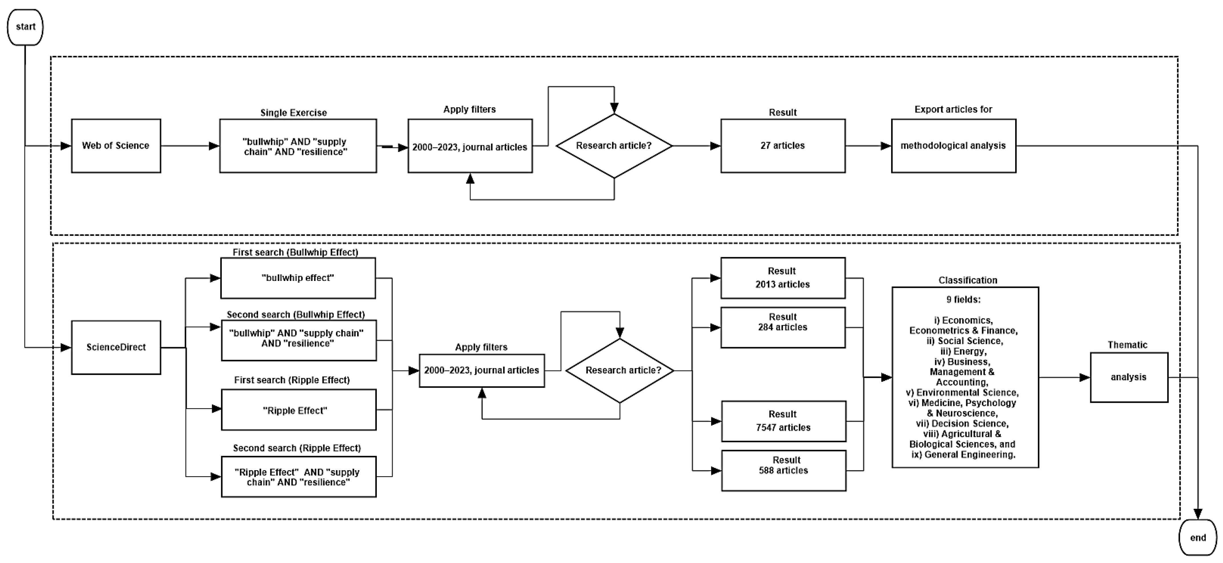
As previously mentioned, this study does not follow a systematic review protocol such as PRISMA, nor does it aim to be exhaustive. Instead, it adopts a hybrid and exploratory approach focused on identifying methodological patterns and disciplinary gaps in the intersection between the Bullwhip Effect, Ripple Effect, and supply chain resilience (SCR). The Web of Science (WoS) database was selected due to its high academic selectivity, indexing standards, and relevance for peer-reviewed, high-impact research. The search was performed using the following keyword combination: “Bullwhip Effect” AND “resilience” AND “supply chain”, covering the time window from 2000 to 2023. This narrow keyword strategy intentionally ensured thematic precision and alignment with the research objectives, even at the cost of volume. The resulting number of articles (n = 27) is not presented as a statistically representative sample of all the SCR literature but as a reflection of the limited existing academic focus on the explicit connection between these phenomena. This scarcity, in itself, is an important finding: it highlights a research gap in modeling resilience from the lens of the Bullwhip and Ripple Effects. Inclusion criteria were as follows: (i) studies published in peer-reviewed journals indexed in WoS, (ii) the explicit treatment of the Bullwhip Effect or Ripple Effect regarding supply chain resilience, and (iii) methodological clarity enabling classification. Exclusion criteria included the following: (i) inaccessible full texts, (ii) articles where resilience was only marginally mentioned, and (iii) studies unrelated to methodological modeling. All selection decisions were made manually, and full-text reading was conducted to verify thematic alignment. While modest in size, this curated dataset is analytically sufficient to detect disciplinary trends and methodological preferences, particularly in the context of nonlinear and adaptive modeling approaches such as those grounded in complex systems or AI.

From this sample, the methodologies used by the authors in this research were analyzed, resulting in the following proposed classification:

4.1.1. Linear Analysis

In the papers by Thomas et al. [30] and Kinra et al. [8], linear approaches were employed to analyze the effects of Bullwhip and Ripple on supply chains, respectively. These linear approaches, based on simulation models and control engineering techniques, make it possible to simplify the inherent complexity of the dynamic systems involved in supply chains. Thomas et al. [30] examined resilience and robustness in relation to the Bullwhip Effect through a production and inventory control model. Through this method, one can detect essential parameters and examine their effects on system behavior during disruptive conditions. Conversely, the work of Kinra et al. [8] developed a linear model to assess the Ripple Effect that allows suppliers to determine their risk exposure without calculating disruption probabilities, enabling them to focus on potential loss sizes. Such approaches generate value by providing an understanding of the system based on the decomposition of complex issues into smaller units over which the contributing factors might be analyzed within the supply chains. The real problem is that it tends to oversimplify the realities of such dynamics, creating a risk of ignoring relevant nonlinear couplings in gaining system insights. The Bullwhip Effect creates barriers to comprehending how differing recovery times affect system resilience. As for the Ripple Effect, simplification might not adequately capture the complexity of global supply networks and the interdependencies between providers.

4.1.2. Nonlinear Analysis

Accompanying articles addressing the analysis of the Bullwhip Effect and the Ripple Effect from a nonlinear perspective used advanced approaches that capture the dynamic complexity and nonlinear interactions in supply chains. Park et al. [9] investigated how disturbance within distributors’ circular flow systems enables an amplification of the Ripple Effect, thereby creating wider recovery spans and further negative fallout relative to disturbances imposed outside of such circular flows. This nonlinear approach is crucial to understanding the spread of disruptions and their impact on supply chain resilience [9]. On the other hand, Badakhshan et al. [1] applied a simulation approach based on system dynamics and genetic algorithms to optimize cash flow management and minimize both the Bullwhip Effect and Bullwhip Cash Flow (CFB) in supply chains. This nonlinear methodological approach has opened up the possibility to capture the inherent complexity within inventory and cash flow decisions. It could serve as a nice tool for liquidity management while helping to achieve a reduction in inefficiencies within the supply chain [1]. In addition, Garvey and Carnovale [31] explored how the complexity and interconnectivity of global supply networks can amplify the Ripple Effect, using dynamic Bayesian networks to model and quantify risk spread. This nonlinear approach allows for the identification of optimal supplier selection and order allocation strategies that mitigate risk and improve global resilience [31]. Pavlov et al. [32] developed a method based on graph theory and structural genomes to model the dispersion of the Ripple Effect and recovery paths, integrating the detection of disruption scenarios and the optimization of reconfiguration paths in complex supply networks. This nonlinear approach makes it possible to analyze how disruptions propagate and affect different parts of the network, taking into account not only the direct connections but also the indirect and latent ones that could amplify the negative effects [32].

4.1.3. Resilience Low-Focus Analysis

Articles that address the analysis of the Bullwhip and Ripple Effects from nonlinear approaches present a relatively weak description in terms of their direct application to supply chain resilience. Although these studies, such as those by Mu et al. [33], Badakhshan et al. [1], and Garvey and Carnovale [31], among others, employed advanced methodologies and complex models to quantify the effects of disruptions on supply chains, they tend to focus more on the theoretical modeling and simulation of the specific effects rather than offering a practical and applicable integration of their findings into resilience strategies for supply chains. Such shortcomings are shown by the poor guidance contained in these articles on specific ways that businesses can adopt their models to be more attuned to resilience against various disruptions. Also, these journal articles do not specify nor discuss in-depth how their model deliverables can be translated into concrete action on either risk mitigation or resilience strengthening, and this is an area of opportunity. The inclusion of practical case studies, implementation approaches, or even specific recommendations for resilience management would greatly allow for the immediate and grounded application of their findings. Thus, as robust as the work by Kinra [8] and other co-authors of 2019 was, the proposed models lack the applicability and sense of direction to enhance real-world supply chain resilience.

While the critique of existing studies in this category is justified—particularly their lack of direct, practical integration with supply chain resilience strategies—it is equally important to provide a constructive alternative. This study addresses that gap by proposing an initial conceptual framework informed by the interdisciplinary signals emerging from our neural network analysis. Specifically, our SHAP-based results and LSTM time-series models consistently highlight Business, Engineering, Environmental Science, and Decision Science as the most influential fields driving resilience-oriented research output. Rather than approaching resilience in isolation or as a theoretical abstraction, we suggest that future models adopt a hybrid interdisciplinary approach that structurally integrates the following: (i) Engineering for system-level modeling and simulation of disruptions; (ii) Business and Decision Sciences for tactical decision-making and inventory policies; (iii) Environmental Sciences for embedding sustainability and external shock resilience (e.g., climate or energy volatility). This integration can enable models that not only capture the complexity of Ripple or Bullwhip dynamics but also translate those dynamics into resilience-enhancing decisions—such as multi-tier supplier optimization, recovery time prediction, or resource reallocation under disruption. Moreover, the patterns revealed by our LSTM-based forecasting provide temporal insights that support anticipatory resilience strategies, where firms can act before vulnerabilities escalate. While this paper does not claim to develop a prescriptive model, it provides an empirically grounded, methodologically explicit roadmap for future research to bridge theoretical modeling with practical resilience applications.

4.1.4. Resilience High-Focus Analysis

The accompanying articles apply a remarkable focus on supply chain resilience, offering several important contributions to the field. For example, Thomas et al. [30] explored the relationship between resilience, robustness, and the Bullwhip Effect through control engineering and simulation techniques, establishing that it is possible to improve resilience and reduce the Bullwhip Effect through an appropriate selection of control parameters. This makes the interrelationship between inventory management and a supply chain recovery from disturbance comprehensible. Looking more closely at some of the key studies in the field reveals just how fragmented the methodological landscape still is. For example, Park et al. [9] used simulation-based network models to study Ripple Effects in supply chains, with a focus on how disruptions spread through different network structures. While their approach does a good job of revealing structural weak points in the network, it falls short when it comes to linking those insights to actual decision-making or control strategies, making it harder to apply in real-world settings. In contrast, Badakhshan et al. focused more on operational control, working to optimize factors like lead times and service levels. Their work offers actionable insights for managers, but it tends to overlook how disruptions Ripple through the broader network or how systems respond over time. Garvey and Carnovale [31] offered a data-driven perspective by assessing risk exposure across supply tiers, but their model lacks dynamic components and assumes relatively static system behaviors. Similarly, Kinra et al. proposed an econometric model to assess exposure levels in global supply chains, yet their work remains isolated from operational resilience modeling or adaptive dynamics. Pavlov et al. [32] contributed a hybrid simulation framework that blends structural modeling with some control logic. However, their model is highly abstract and complex to operationalize in real-time decision environments. Ivanov [32], a key contributor to the digital supply chain resilience literature, introduced the concept of the “Ripple Effect” in dynamic settings using discrete-event and hybrid simulation; however, his models often prioritize scenario coverage over model parsimony, raising concerns about generalizability.

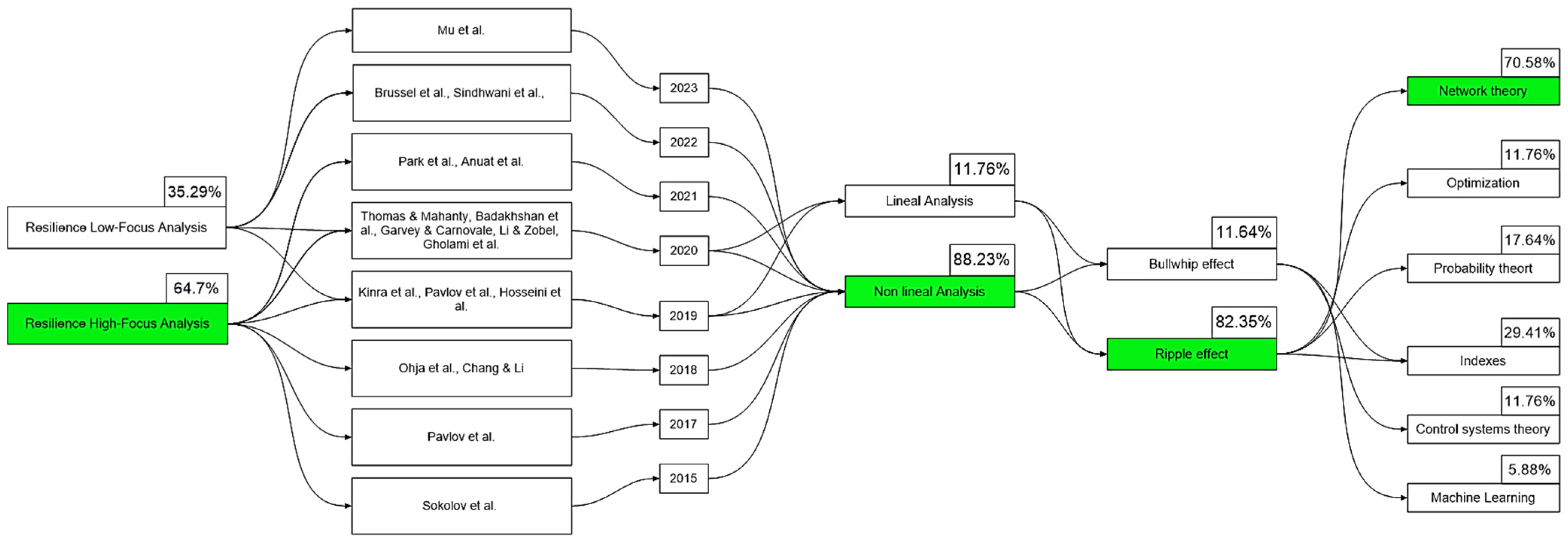
Altogether, these studies paint a picture of a fragmented field. Some focus on network structures, others on optimization or statistical risk assessment—but very few try to bring these perspectives together into a single, cohesive modeling approach. Even though they often tackle similar problems, they tend to work in isolation, each within its own disciplinary framework, without engaging with one another’s assumptions or methods. This lack of connection makes it harder to build cumulative knowledge and slows the development of practical, flexible tools that supply chains can actually use to manage disruptions. Our study identifies this methodological dispersion and calls for integrative modeling approaches that bridge structural dynamics, control systems, and uncertainty management in the context of Bullwhip and Ripple Effects under a resilience lens. Finally, the aforementioned analysis is succinctly and clearly summarized in Table 2 and Figure 6.

Figure 6. Classification of methodologies and modeling approaches in supply chain resilience studies from 2000 to 2023. The diagram shows the distribution of articles by year, focus on resilience (low vs. high), analytical approach (linear vs. nonlinear), type of effect studied (Bullwhip or Ripple), and dominant modeling technique. Source: Authors’ own work, based on [1,6,8,9,10,11,12,30,31,32,33,34,35,36,37].

Figure 6. Classification of methodologies and modeling approaches in supply chain resilience studies from 2000 to 2023. The diagram shows the distribution of articles by year, focus on resilience (low vs. high), analytical approach (linear vs. nonlinear), type of effect studied (Bullwhip or Ripple), and dominant modeling technique. Source: Authors’ own work, based on [1,6,8,9,10,11,12,30,31,32,33,34,35,36,37].

Table 2. Modeling framework and applied techniques. The classification of studies as having a “low application in resilience” was based on a qualitative assessment through the direct reading and observation of each article. Studies were considered to have low application if their resilience analysis was broad and general rather than explicitly focused on supply chain resilience. Only those articles that deeply examined resilience within supply chain contexts were categorized as having a high application. A checkmark (✔) indicates that the corresponding study explicitly addresses the Bullwhip or Ripple effect. Source: Authors’ own work.

Author	Year	Nonlinear	Bullwhip	Ripple	Resilience Approach	Technique
Mu et al. [33]	2023	yes		✔	Low	Network topology
Brusset et al. [34]	2022	yes		✔	Low	Susceptible–Infected–Susceptible (SIS)
Sindhwani et al. [12]	2022	yes		✔	Low	Bayesian network
Park et al. [9]	2021	yes		✔	High	Real-world data and structures/discrete event simulation models (DESMs)
Anuat et al. [37]	2021	yes		✔	High	Bayesian network/Markov chains
Thomas et al. [30]	2020	no	✔		High	Inventory- and order-based production control system (IOBPCS)
Badakhshan et al. [1]	2020	yes	✔		Low	Genetic algorithms/Beer game
Garvey and Carnovale [31]	2020	yes		✔	Low	Bayesian network
Li and Zobel [6]	2020	yes		✔	High	Topological analysis
Gholami-Zanjani et al. [35]	2020	yes		✔	High	Monte Carlo/entire mixed programming
Kinra et al. [8]	2019	no		✔	Low	Indexes
Pavlov et al. [38]	2019	yes		✔	High	Genome method
Hosseini et al. [36]	2019	yes		✔	High	Bayesian network/Markov chains
Ojha et al. [11]	2018	yes		✔	High	Bayesian network/indexes
Chang and Li [39]	2018	yes	✔		High	Model APIOBPCS (Adjusted Production Inventory Order Based on Production) Capacity System)
Pavlov et al [32]	2017	yes		✔	High	Hybrid fuzzy–probabilistic approach
Sokolov et al. [10]	2015	yes		✔	High	Method AHP (Analytic Hierarchy Process)

Table 2. Modeling framework and applied techniques. The classification of studies as having a “low application in resilience” was based on a qualitative assessment through the direct reading and observation of each article. Studies were considered to have low application if their resilience analysis was broad and general rather than explicitly focused on supply chain resilience. Only those articles that deeply examined resilience within supply chain contexts were categorized as having a high application. A checkmark (✔) indicates that the corresponding study explicitly addresses the Bullwhip or Ripple effect. Source: Authors’ own work.

Author	Year	Nonlinear	Bullwhip	Ripple	Resilience Approach	Technique
Mu et al. [33]	2023	yes		✔	Low	Network topology
Brusset et al. [34]	2022	yes		✔	Low	Susceptible–Infected–Susceptible (SIS)
Sindhwani et al. [12]	2022	yes		✔	Low	Bayesian network
Park et al. [9]	2021	yes		✔	High	Real-world data and structures/discrete event simulation models (DESMs)
Anuat et al. [37]	2021	yes		✔	High	Bayesian network/Markov chains
Thomas et al. [30]	2020	no	✔		High	Inventory- and order-based production control system (IOBPCS)
Badakhshan et al. [1]	2020	yes	✔		Low	Genetic algorithms/Beer game
Garvey and Carnovale [31]	2020	yes		✔	Low	Bayesian network
Li and Zobel [6]	2020	yes		✔	High	Topological analysis
Gholami-Zanjani et al. [35]	2020	yes		✔	High	Monte Carlo/entire mixed programming
Kinra et al. [8]	2019	no		✔	Low	Indexes
Pavlov et al. [38]	2019	yes		✔	High	Genome method
Hosseini et al. [36]	2019	yes		✔	High	Bayesian network/Markov chains
Ojha et al. [11]	2018	yes		✔	High	Bayesian network/indexes
Chang and Li [39]	2018	yes	✔		High	Model APIOBPCS (Adjusted Production Inventory Order Based on Production) Capacity System)
Pavlov et al [32]	2017	yes		✔	High	Hybrid fuzzy–probabilistic approach
Sokolov et al. [10]	2015	yes		✔	High	Method AHP (Analytic Hierarchy Process)

While the linear/nonlinear and resilience-focused classifications are conceptually distinct, they intersect in important ways. Some studies employ advanced modeling techniques yet offer limited insights into resilience mechanisms, while others prioritize resilience but use basic linear tools. To address this overlap, a combined classification matrix was created to map how methodological complexity aligns with resilience depth across the literature. This structure helps clarify where the field is concentrated—and where future integration is needed. To address the reviewer’s concern regarding potential overlap between resilience focus and modeling type,

Table 3. Cross-classification of reviewed studies by modeling approach and resilience focus.

Modeling Approach	Low Resilience Focus	High Resilience Focus
Linear Models	Kinra et al. [8]	Thomas and Mahanty [30]
Nonlinear Models	Badakhshan et al. [1]; Garvey and Carnovale [31]; Mu et al. [33]; Brusset et al. [34]; Sindhwani et al. [12].	Park et al. [9]; Li and Zobel [6]; Gholami-Zanjani et al. [35]; Pavlov et al. [32]; Pavlov et al. [38]; Hosseini et al. [36]; Ojha et al. [11]; Chang and Li [39]; Sokolov et al. [10]

presents a simplified cross-classification to visualize this relationship more clearly.

Beyond descriptive classification, the reviewed literature reveals several important analytical insights regarding the methodological landscape of Bullwhip and Ripple Effects in the context of supply chain resilience. First, the clear prevalence of nonlinear approaches (88.23%)—notably simulation, system dynamics, Bayesian networks, and network theory—highlights the consensus that supply chain disruptions are inherently complex and path-dependent. However, this methodological preference also exposes a bias toward computational sophistication, which, while capturing systemic interdependencies, often lacks practical translatability for decision-makers. For instance, studies like Park et al. [9] and Pavlov et al. [32] demonstrate advanced network-based or genome-based modeling yet offer limited operational strategies or policy-level applications.

In contrast, linear models such as those by Thomas et al. [30] or Kinra et al. [8], despite their simplicity, offer more direct implications for managerial control systems (e.g., inventory tuning and exposure assessment), particularly in environments with limited data or operational constraints. This dichotomy suggests a methodological gap in hybrid modeling, where analytical tractability and practical relevance are balanced—an opportunity scarcely addressed in the reviewed literature. Moreover, from the disciplinary perspective, the methodological choices seem to correlate with the originating academic fields: Engineering and Decision Sciences, which dominate the sample, tend to favor nonlinear, simulation-based, or control-theoretic methods. Meanwhile, contributions from Economics or Business lean more toward index-based or optimization-driven frameworks. This points to an opportunity for the cross-pollination of methodological paradigms, as few studies attempt to integrate, for example, econometric and system-dynamic approaches into a unified resilience framework.

Lastly, the bibliometric data show that while 64.7% of studies address resilience with a high conceptual focus, the Bullwhip Effect appears underexplored in this domain, comprising only 11.7% of the resilience-oriented studies. This is especially surprising considering the Bullwhip Effect’s foundational role in supply chain instability. The disproportionate focus on the Ripple Effect may reflect its more visible propagation dynamics, but it also suggests a need to reframe the Bullwhip Effect not just as a demand distortion but as a structural vulnerability within resilience strategies. In sum, this classification exercise not only organizes methodological choices but surfaces critical gaps and disciplinary silos that constrain the advancement of integrative, actionable resilience modeling.

4.2. Analysis of Quantitative Results

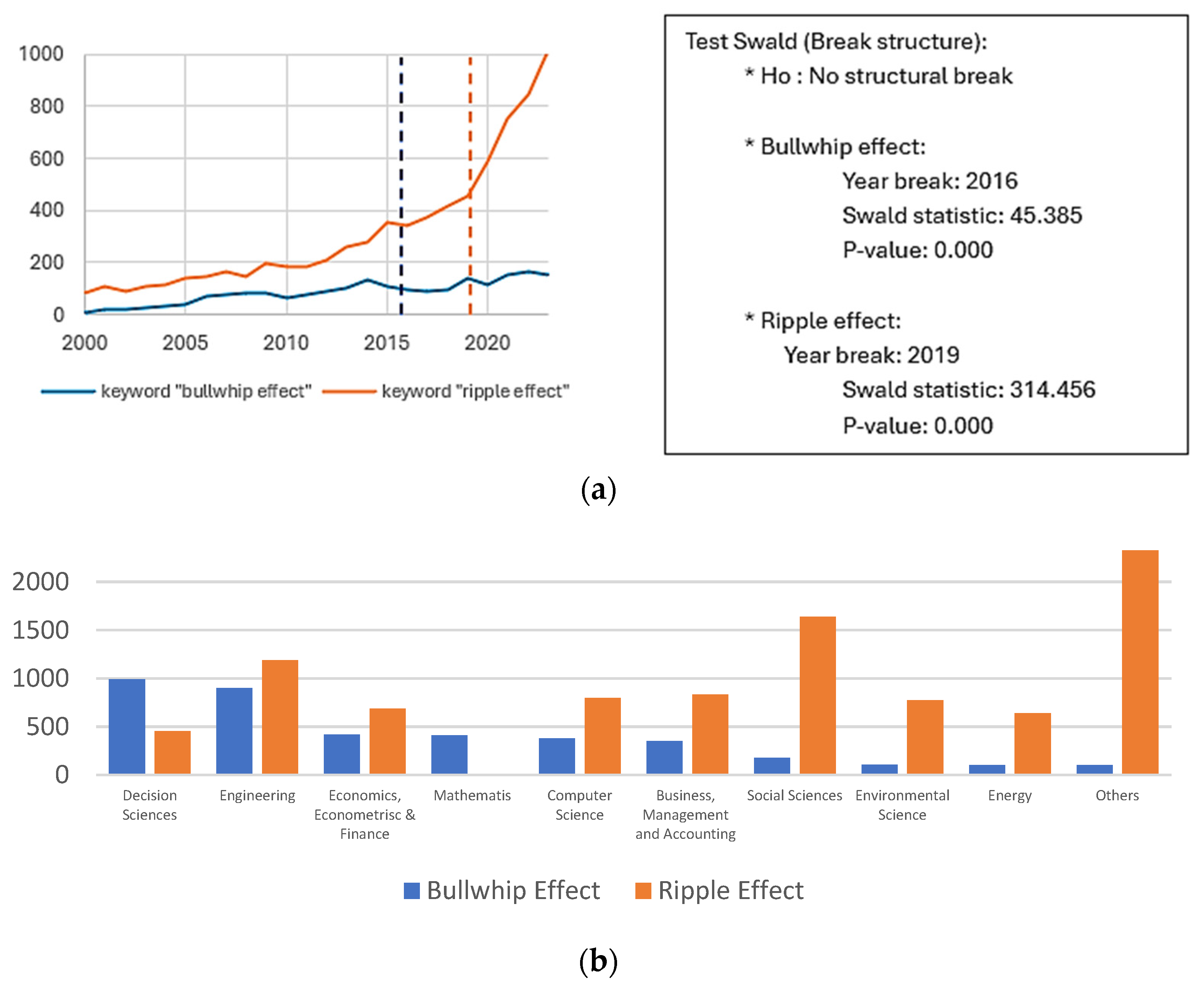
Figure 7a,b illustrate the trends in the volume of research conducted on the Bullwhip and Ripple Effects (in general scope, first exercise) from 2000 to 2023, along with the extent of its connections to various fields of study, based on the filtered results from the selected databases [24]. Similarly, Figure 7a,b depict the trends for research specifically focusing on the relationship between the Bullwhip Effect, Ripple Effect, and the Resilience Effect in supply chains.

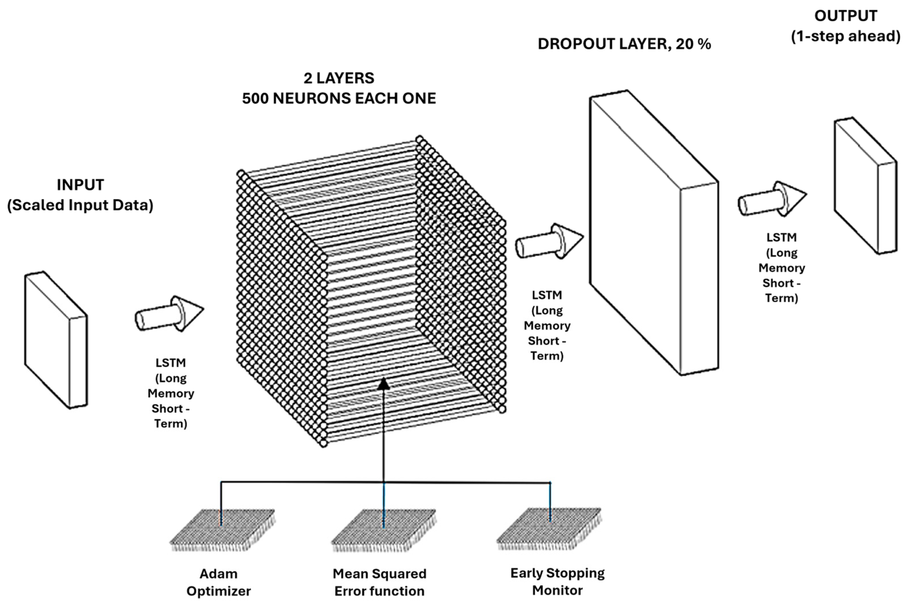
The quantitative analysis in Section 3.2 employs several statistical techniques to validate the robustness of time-series trends and to detect significant structural changes in research dynamics. One of the main tools used is the Wald-type test for structural breaks, implemented through the “Swald” procedure available in Stata. This test is designed to identify statistically significant shifts in the behavior of a time series (e.g., in publication volume) by evaluating changes in model coefficients at unknown breakpoints. The assumptions for this test include a minimum number of observations on either side of the potential break, the stationarity of residuals, and independence across time lags. Results are considered significant if the null hypothesis of no structural break is rejected at common significance levels (1%, 5%, 10%). In addition to the Swald test, the analysis includes the following: normality tests, Augmented Dickey–Fuller (ADF) tests to assess stationarity, Bartlett’s test to evaluate residual autocorrelation, and the Variance Inflation Factor (VIF) to test for multicollinearity. These were applied to ensure that the LSTM model was built on a statistically reliable time series. All variables were log-transformed and normalized before testing to meet the distributional assumptions.

The approach’s limitations include the relatively short time series in some disciplinary categories, the potential sensitivity of the Swald test to noise and sample size, and the lack of causal modeling due to the exploratory nature of the data. However, the combination of structural break detection and time-series diagnostics provides a strong foundation for interpreting trend discontinuities as meaningful shifts in research focus. Full model specifications and the Stata/Python code are available from the authors upon request.

Figure 7a highlights the significant growth in the production of scientific articles, using “Bullwhip Effect” and “Ripple Effect” as the keywords, over the past two decades. Notably, the year 2016 marked a pivotal point in this upward trend for the Bullwhip Effect, as confirmed by the Swald test, which showed high statistical significance; and the year 2019 for the Ripple Effect tipping point (critical values were determined based on the chi-square distribution at conventional significance levels (1%, 5%, and 10%); the reported p-values indicate whether the null hypothesis of no structural break can be rejected). This suggests that the interest in studying the Bullwhip Effect has remained consistently strong, particularly considering its initial discovery in the 1960s [3]. In 2016, some momentous global events helped to shape the Economic and Business landscape: the UK leaving the European Union (Brexit) in June created market uncertainty and raised fears about future trade relationships; the election of Donald Trump as President of the United States shifted global trade and regulatory policies, notably leading to the abandonment of the Trans-Pacific Partnership; in its transition to a consumption-driven economy, China’s economic slowdown sharpened global commodity markets; the crude oil prices engendered timid recoveries after their previous turmoil, an event impacting equally on exporters and importers; at last, in the crevice of the refugee crisis in Europe, ignited by the conflicts in the Middle East, the wheels of the smoke and labor systems in the region were further clogged. These events seem to have greatly influenced the explosion of Bullwhip Effect studies, as indicated by the structural break identified in the Swald test.

Similarly, Figure 8a illustrates the production volume of scientific articles where “Bullwhip Effect”, “Ripple Effect”, “resilience”, and “supply chain” are used as keywords, showing remarkable exponential growth in this interdisciplinary area. As indicated by the Swald test, which found a structural break in 2019, which served as a major catalyst for this surge in research output for Bullwhip and Ripple Effects: the year 2019 witnessed several significant economic and logistical events globally (critical values were determined based on the chi-square distribution at conventional significance levels (1%, 5%, and 10%); the reported p-values indicate whether the null hypothesis of no structural break can be rejected). The U.S.–China trade war intensified, imposed tariffs, and disrupted supply chains all over the world, particularly for industries that rely heavily on Chinese manufacturing. Brexit in the United Kingdom created a cloud of uncertainty over Europe’s trade and logistics landscape due to companies rushing to prepare for possible border delays and regulatory changes. A slowdown of the global economy with a waning growth of major regions in Europe and Asia. The technological revolution continued its onslaught in transforming logistics, with automation and AI increasingly embraced in warehouses and the growth of e-commerce fueling demand for efficient last-mile delivery solutions. Additionally, sustainability became a focal point, with businesses implementing greener supply chain practices to address environmental concerns.

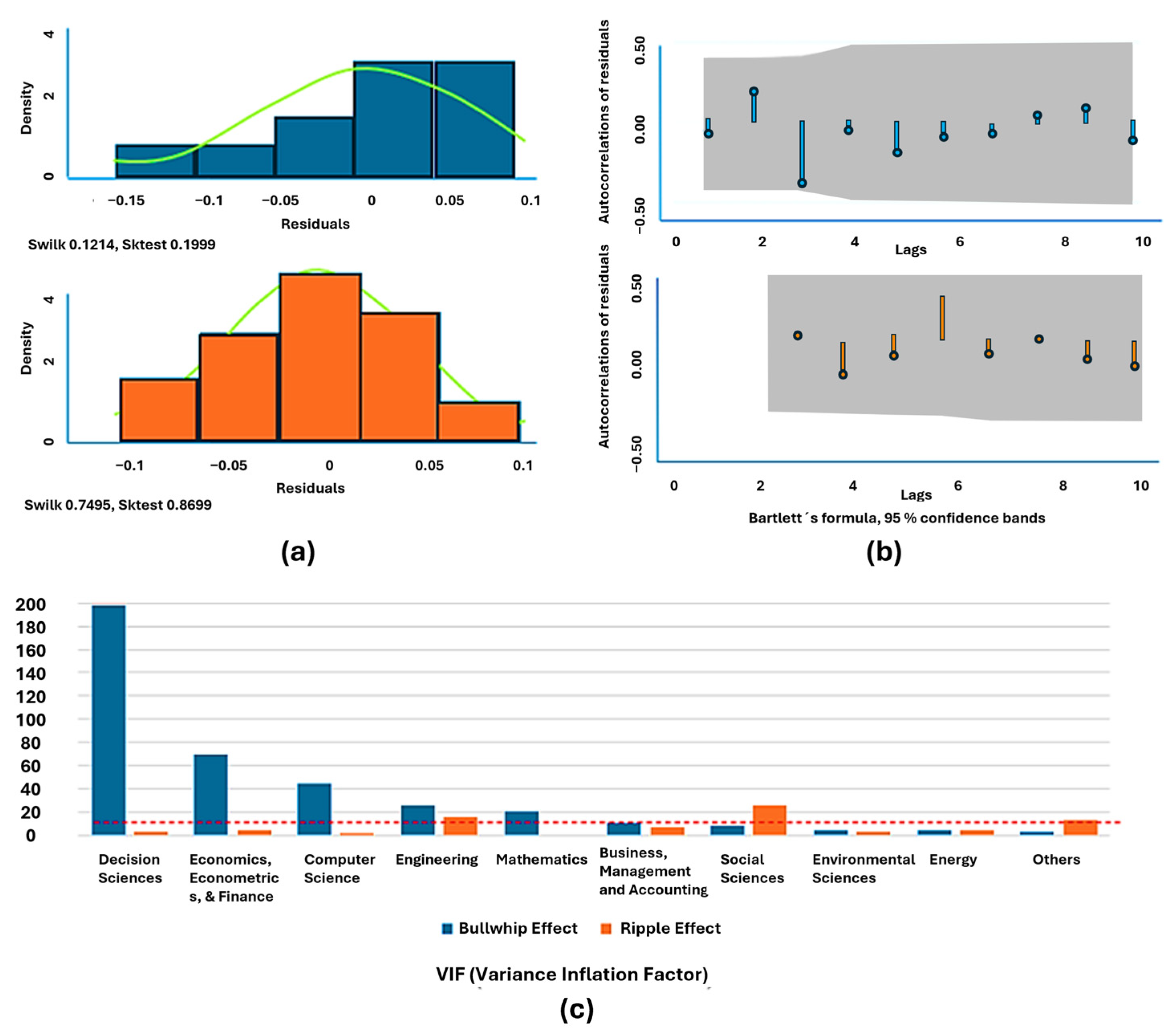
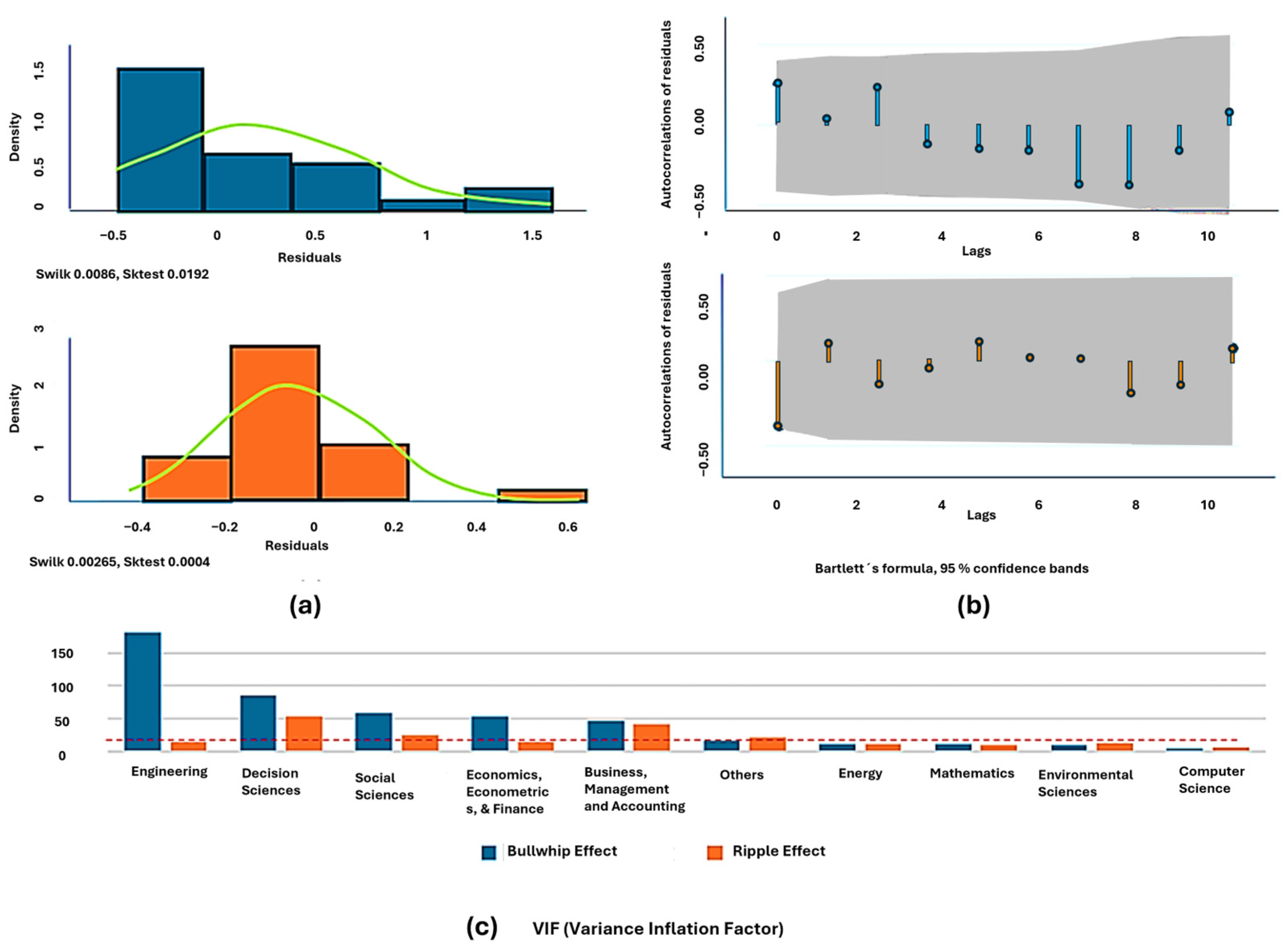
A notable finding from the results is the strong connection of this interdisciplinary field not only with economic sciences, typically associated with the Bullwhip and Ripple Effects, but also with Engineering and Decision Sciences. Figure 8b highlights that the highest-ranked academic areas in the collected data include Engineering and Decision Science alongside Business, Mathematics, Economics, Social Sciences, Environmental, Computer, Energy, and others. This suggests that applied Engineering Sciences play a critical role in the study of the Bullwhip Effect in its general scope. For the quantitative analysis, a series of tests were conducted on the collected time series to ensure their statistical robustness, checking for probabilistic distribution, multicollinearity, autocorrelation, and stationarity. High multicollinearity was found in the variables, as confirmed by the Variance Inflation Factor test (Figure 9c). The Augmented Dickey–Fuller unit root test (

Table 4. Augmented Dickey–Fuller unit root test, 1st exercise. Augmented Dickey–Fuller (ADF) unit root test results for Bullwhip and Ripple Effects, assessing stationarity of variables. This table presents ADF test results for various variables under Bullwhip and Ripple conditions. The test evaluates stationarity, with significant p-values indicating that most variables are stationary, while a few remain non-stationary in the Ripple scenario. Includes trending term; p-value: *** < 0.01; ** < 0.05; * < 0.1; “n.a.” (not applicable) indicates that no stationary value was found for the variable, making it methodologically invalid to estimate lags or apply Z(t) transformations. “---” indicates that no observations were available for the variable Z_t in the dataset, and thus, no statistical test could be applied. Source: Authors’ own work.

	Bullwhip	Ripple	Bullwhip	Ripple	Bullwhip	Ripple	Bullwhip	Ripple
Variable	Z(t) (ADF)	Z(t) (ADF)	MacKinnon p-Value		Lags		Conclusion
${lny}_t$	−6.956 ***	n.a.	0.0000	n.a.	0	n.a.	Stationary	Non-stationary
${lnW}_t$	−8.038 ***	−3.576 **	0.0000	0.0319	0	0	Stationary
${lnP}_t$	−8.020 ***	−7.166 ***	0.0000	0.0000	0	0	Stationary
${lnH}_t$	−4.005 **	−4.476 ***	0.0087	0.0017	0	0	Stationary
${lnE}_t$	−3.843 **	−5.099 ***	0.0145	0.0001	0	0	Stationary
${lnZ}_t$	−10.208 ***	---	0.0000	---	0	---	Stationary	---
${lnB}_t$	−4.138 **	n.a.	0.0055	n.a.	0	n.a.	Stationary	Non-stationary
${lnK}_t$	−5.820 ***	−4.039 **	0.0000	0.0077	0	0	Stationary
${lnG}_t$	−3.278 *	n.a.	0.0699	n.a.	0	n.a.	Stationary	Non-stationary
${lnM}_t$	−5.089 ***	−6.633 ***	0.0001	0.0000	0	0	Stationary
${lnN}_t$	−5.244 ***	−4.246 **	0.0001	0.0038	2	0	Stationary

) confirmed non-stationarity only in one variable. To address these problems, the neural network model was chosen, which effectively handles both multicollinearity and non-stationary series. Preliminary results showed a Gaussian distribution of residuals, supported by normality tests (Swilk and Sktest in Stata 15.0 [40]), and acceptable results in Bartlett’s autocorrelation test, remaining within the 95% confidence range as lags increased (Figure 9b).

Thus, after implementing the adjustments suggested by the preliminary statistical tests, the final reduction in the model for the first exercise is ((2) and (3)):

$$\begin{gathered} \left(\mathrm{Bullwhip}\right) \Rightarrow {lny}_{1t}={{\alpha }_{1}lnW}_t+{\alpha }_{2}ln{P}_t+{\alpha }_{3}ln{H}_t+{\alpha }_4{lnE}_t+{\alpha }_5{lnZ}_t+ \\ {\alpha }_6{lnB}_t+{\alpha }_7{lnK}_t+{\alpha }_8{lnG}_t+{\alpha }_9{lnM}_t+{\alpha }_{10}{lnN}_{t-2}+\epsilon \end{gathered}$$

(2)

$$\begin{gathered} \left(\mathrm{Ripple}\right) \Rightarrow { lny}_{1t}={\alpha }_1{lnW}_t+{\alpha }_{2}ln{P}_t+{\alpha }_{3}ln{H}_t+{\alpha }_4{lnE}_t+{\alpha }_5{lnZ}_t+ \\ {\alpha }_6{lnB}_t+{\alpha }_7{lnK}_t+{\alpha }_8{lnG}_t+{\alpha }_9{lnM}_t+{\alpha }_{10}{lnN}_t+\epsilon \end{gathered}$$

(3)

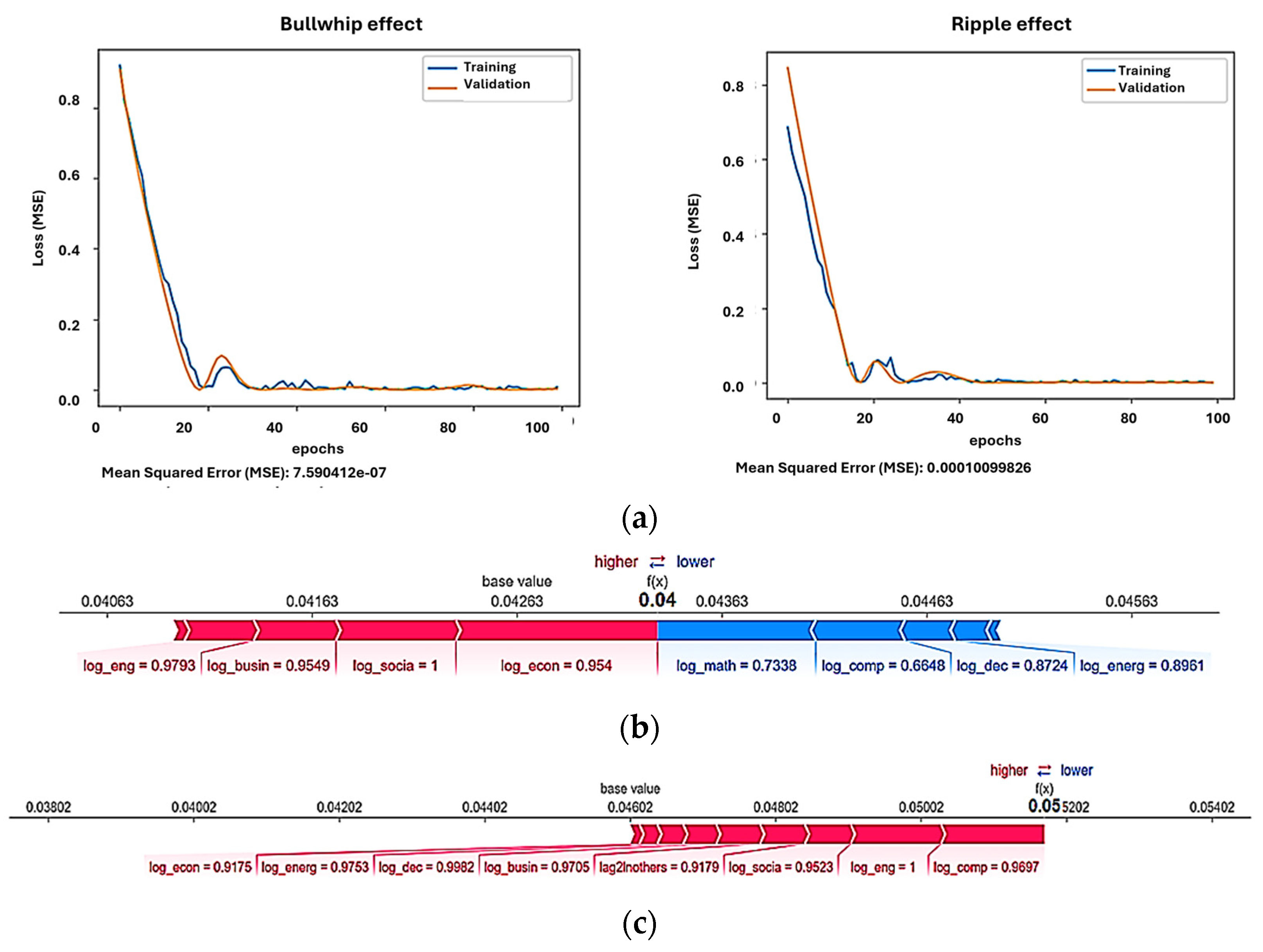
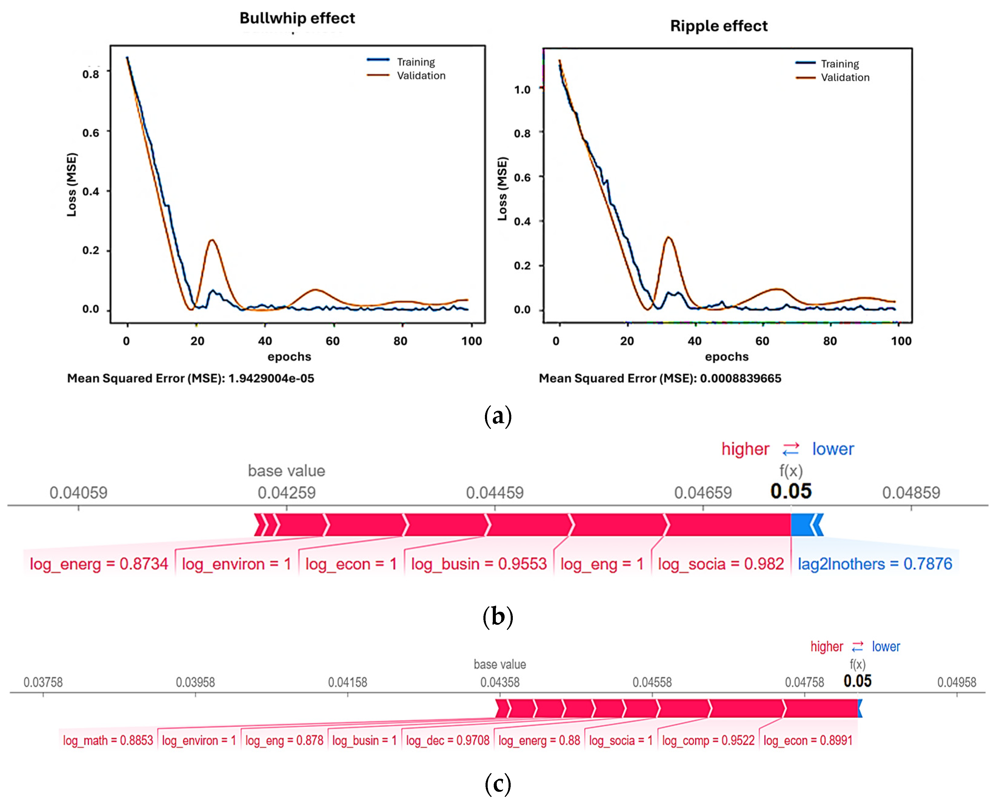
Figure 10a shows the loss during both training and validation across 100 epochs, with Mean Squared Error (MSE) as the metric. We observe that both curves decrease rapidly in the first 20 epochs, indicating effective learning during this initial phase. However, after epoch 20, the MSE stabilizes and exhibits a slight increase in fluctuation. The validation curve closely follows the training curve, which suggests that the model generalizes well and that there is minimal overfitting. Model performance was assessed using standard metrics. For the Bullwhip Effect model, the final Mean Squared Error (MSE) on the validation set was 7.59 × 10⁻⁷, while the Ripple Effect model achieved an MSE of 1.009 × 10⁻⁴ (see Figure 10a). Both models converged after approximately 30–40 epochs, and validation loss remained stable across the training window, indicating strong generalization. While LSTM models do not rely on R² in the same way as traditional regression models, supplementary estimation yielded approximate R² values above 0.85 for both cases, suggesting solid predictive accuracy. In addition, the 80/20 time-based train–validation split, combined with early stopping and low learning rate tuning, helped prevent overfitting, as reflected in the close alignment of training and validation error curves.

Figure 10b is a SHAP (Shapley Additive Explanations) force plot, which reveals the individual feature contributions to a particular average output. SHAP (Shapley Additive Explanations) was applied to interpret variable importance in the LSTM neural network model used for bibliometric trend analysis. This approach was chosen due to its ability to provide transparent, feature-level contributions in complex, nonlinear models. To ensure robustness, SHAP results were compared with alternative feature importance methods (e.g., permutation importance) and exhibited consistent patterns, reinforcing its validity for this context. Given SHAP’s widespread use in deep learning explainability, its application here is methodologically justified. Here, for the Bullwhip Effect, study fields like Economics and Social are pushing the prediction value higher (shown in red), while variables such as Mathematics and Computation are pushing it lower (shown in blue). This demonstrates that certain variables like Economics and Social Sciences have a more significant positive effect, indicating a strong correlation with the target of the Bullwhip Effect. Conversely, the technical fields such as Mathematics, Computation, Decision, and Energy Sciences contribute less, or even negatively, suggesting that their influence on the model is less direct in this scenario. For the case of the Ripple Effect, Figure 10c shows that Computation and Engineering Science are the strongest contributors to the predicted value in the model.

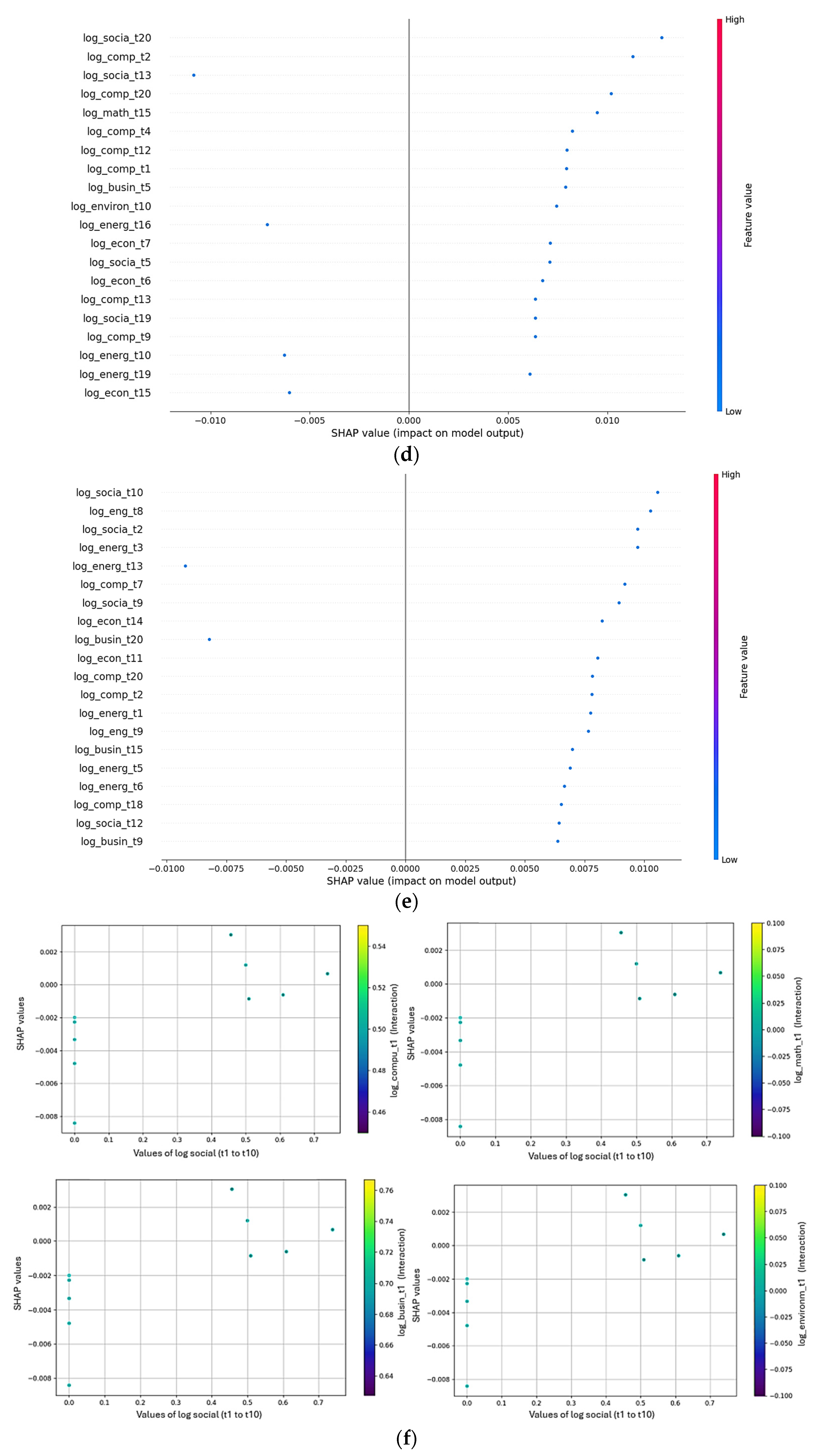
Figure 10d,e present a SHAP summary plot, which ranks the features by their impact on the model output across all observations. The top features, such as Energy, Environment, and Business, show the highest influence on the Bullwhip Effect in its general scope and Business, Environment, and Energy, for the Ripple Effect scope. Interestingly, the presence of multiple time-lagged features from the same categories suggests that Energy has a temporal and cumulative impact on the prediction. Moreover, features with higher SHAP values (closer to the right) have a more substantial positive effect on the model outcome, while those on the left may contribute less or negatively.

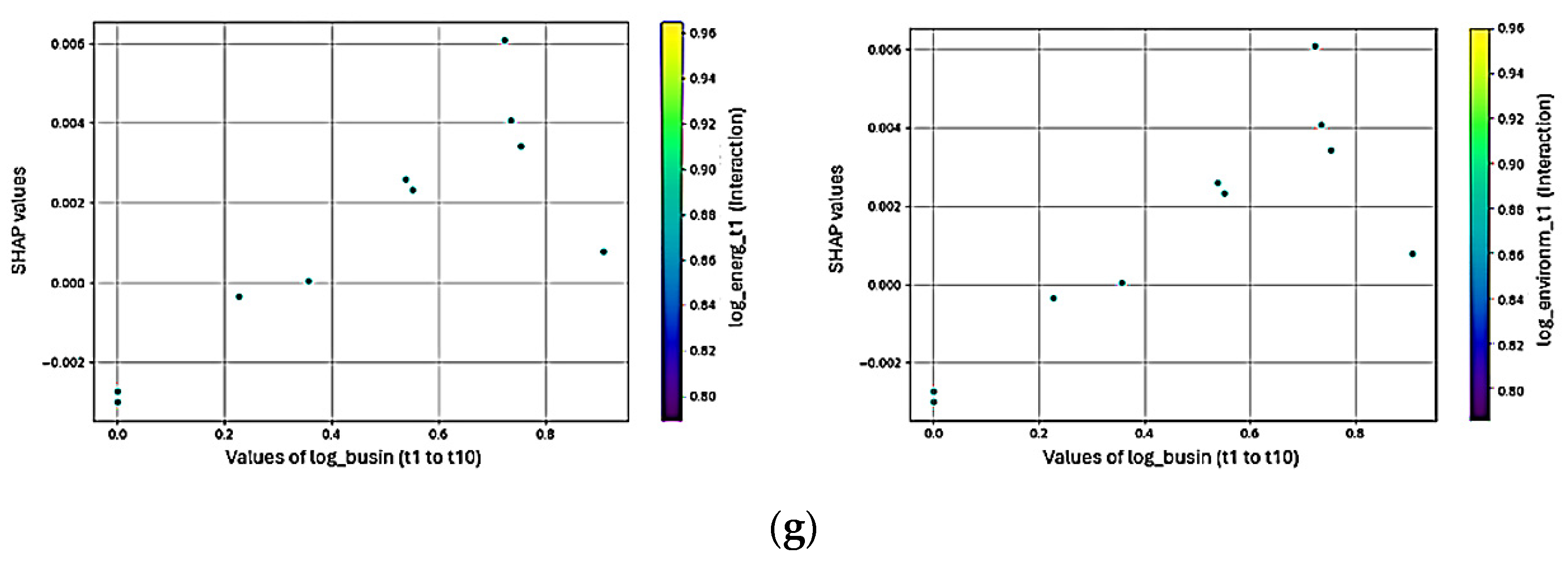
In Figure 10f, the SHAP dependency plot shows how the Energy interacts with the model’s predictions and with the rest of the Bullwhip Effect’s most important variables (Social, Business, Environment, Computation Sciences), and Figure 10g shows the Ripple Effect’s ones (Business, Energy, Environment). For the Bullwhip Effect results, the Energy variable demonstrates a nonlinear relationship with SHAP values; additionally, the variable Energy has an important influence from the Business and Environment variables on its higher values. For the case of the Ripple Effect, Figure 10g shows that its most important variable (Business) has a higher influence than the Energy and Environment variables, implying that sustainability plays an important role in this Ripple phenomenon.

For the second exercise, assessing the interdisciplinary relationship between the Bullwhip and Resilience Effects in supply chains, the same model was applied, with research volume as the dependent variable. Statistical reliability tests included a multicollinearity check (VIF, Figure 11c), revealing high multicollinearity, and an Augmented Dickey–Fuller test (

Table 5. Augmented Dickey–Fuller unit root test, 2nd exercise. Augmented Dickey–Fuller (ADF) unit root test results for Bullwhip and Ripple Effects, assessing stationarity of variables. This table presents ADF test results for various variables under Bullwhip and Ripple conditions. The test evaluates stationarity, with significant p-values indicating that most variables are stationary, while a few remain non-stationary in the Ripple scenario. Includes trending term; p-value: *** < 0.01; ** < 0.05; * < 0.1 “n.a.” (not applicable) indicates that no stationary value was found for the variable, making it methodologically invalid to estimate lags or apply Z(t) transformations. “---” indicates that no observations were available for the variable Z_t in the dataset, and thus, no statistical test could be applied. Source: Authors’ own work.

	Bullwhip	Ripple	Bullwhip	Ripple	Bullwhip	Ripple	Bullwhip	Ripple
Variable	Z(t) (ADF)	Z(t) (ADF)	MacKinnon p-Value		Lags		Conclusion
${lny}_t$	−5.478 ***	−4.60 ***	0.0000	0.0010	0	0	Stationary
${lnW}_t$	−3.377 *	−4.868 ***	0.0545	0.0004	0	0	Stationary
${lnP}_t$	−3.569 *	−5.127 ***	0.0326	0.001	0	0	Stationary
${lnH}_t$	−6.311 ***	−3.388 *	0.0000	0.0531	0	0	Stationary
${lnE}_t$	n.a.	−3.334 *	n.a.	0.0608	n.a.	1	Non-stationary	Stationary
${lnZ}_t$	−4.178 **	−5.859 ***	0.0048	0.000	0	0	Stationary
${lnB}_t$	−3.857 **	n.a.	0.0139	n.a.	0	n.a.	Stationary	Non-stationary
${lnK}_t$	−3.657 *	n.a.	0.0253	n.a.	0	n.a.	Stationary	Non-stationary
${lnG}_t$	−4.490 ***	−3.639 **	0.0016	0.0267	0	0	Stationary
${lnM}_t$	−4.103 **	−4.362 **	0.0062	0.0025	1	0	Stationary
${lnN}_t$	−4.494 ***	−3.919 **	0.0015	0.0114	0	0	Stationary

), which identified one irreversibly non-stationary variable. Various linear and nonlinear models were tested but proved insignificant, leading to the adoption of a neural network to handle non-stationary time series and multicollinearity. Residual tests confirmed a non-Gaussian distribution (Figure 11a), and an autocorrelation test via Bartlett’s procedure showed good results within the 95% confidence level for several lags (Figure 11b).

Finally, after implementing the adjustments suggested by the preliminary statistical tests, the final reduction in the model for the first exercise is ultimately as follows ((4) and (5)):

$$\begin{gathered} \left(\mathrm{Bullwhip}\right) \Rightarrow {lny}_{2t}={lnW}_t+ln{P}_t+ln{H}_t+{lnE}_t+{lnZ}_t+ln\mathrm{B}+ln\mathrm{K}+ \\ {lnG}_t+{lnM}_{t-1}+{lnN}_t \end{gathered}$$

(4)

$$\begin{gathered} \left(\mathrm{Ripple}\right) \Rightarrow {lny}_{2t}={lnW}_t+ln{P}_t+ln{H}_t+{lnE}_{t-1}+{lnZ}_t+ln\mathrm{B}+ln\mathrm{K}+ \\ {lnG}_t+{lnM}_t+{lnN}_t \end{gathered}$$

(5)

Figure 12a illustrates the loss for both training and validation over 100 epochs, using Mean Squared Error (MSE) as the evaluation metric. Notably, both curves decline rapidly within the first 20 epochs, indicating efficient learning during this early phase. After epoch 20, however, the MSE levels off and shows minor fluctuations. The validation curve closely follows the training curve, indicating that the model has generalized well and has undergone insignificant overfit. This close alignment also implies that the model has detected a steady trend in the data. Model performance was assessed using standard metrics. For the Bullwhip Effect model, the final Mean Squared Error (MSE) on the validation set was 1.94 × 10⁻⁵, while the Ripple Effect model achieved an MSE of 8.83 × 10⁻⁴ (see Figure 12a). Both models converged after approximately 30–40 epochs, and validation loss remained stable, indicating good generalization. While LSTM models do not require R² in the same way as regression models, supplementary estimation yielded approximate R² values above 0.85 for both cases, suggesting strong predictive power. Additionally, the train–validation split (80/20) and the use of early stopping helped prevent overfitting, as reflected in the alignment between the training and validation loss curves.

Figure 12b presents a SHAP (Shapley Additive Explanations) force plot, which highlights the individual feature contributions to a specific model output (average value of 0.05). In this plot, fields such as Social, Engineering, and Business Sciences are principally driving the prediction value upward (represented in red) for the Bullwhip Effect, while variables like others are pulling it downward (represented in blue). In the same way, fields such as Economics, Computation, and Social Sciences are the principal positive drivers for the Ripple Effect, without any field working against its positive behavior (Figure 12c).

Figure 12c displays a SHAP summary plot, ranking the features based on their overall impact on the model output across all observations. The most influential features, such as Social and Computational, exhibit the strongest effects on the model’s performance in the general scope. Notably, the appearance of several time-lagged features from the same categories suggests that Computational has both a temporal and cumulative influence on the prediction. Additionally, features with higher SHAP values (closer to the right) contribute more positively to the model’s outcome, whereas those positioned on the left tend to have lesser or even negative contributions. For the case of the Ripple Effect, the most influential fields seem to be the Social, Business, and Energy fields (Figure 12e).

In Figure 12f, the SHAP dependency plot illustrates how the Social variable interacts with the model’s predictions and the other key variables (Mathematics, Environment, Computation Sciences). The Social variable shows a nonlinear relationship with the SHAP values, indicating that its influence on the outcome changes as its values rise. Figure 12g reveals that the Business and Energy fields are the most influential drivers for the principal pivot of the Ripple Effect within the supply chains, the Social field.

Interdisciplinary Influence and SHAP Interpretability

Beyond static importance, SHAP also revealed temporal and relational patterns, offering further insights into the evolving disciplinary structure of resilience research.

To enhance the transparency and explainability of the LSTM predictions, SHAP (Shapley Additive Explanations) was applied as a post hoc interpretability method. SHAP is particularly suitable for this context as it provides individualized, model-agnostic attributions of feature contributions, even in highly nonlinear and temporally sensitive models such as LSTM [27,28]. This allows not only a clearer understanding of which disciplinary variables influenced predictions at different time steps but also deeper insights into the interdisciplinary structure of resilience-focused research on the Bullwhip and Ripple Effects.

The SHAP force plots (Figure 12b,c) revealed that the Bullwhip model was most influenced by contributions from Social Sciences, Engineering, and Business, whereas categories grouped as other (including niche disciplines or uncategorized fields) had a dampening effect on the predicted publication volume. This is consistent with how the Bullwhip Effect is typically explored—as an operational issue tied to process efficiency, organizational routines, and demand fluctuations [8,30]. By comparison, the Ripple model revealed a distinctly different disciplinary emphasis.

Economics, Computer Science, and Social Sciences emerged as the most influential drivers, indicating a stronger theoretical and systems-oriented foundation. This reflects how the Ripple Effect, as a cascading and network-based disruption phenomenon, attracts attention from fields concerned with macro-level modeling, risk propagation, and the simulation of interdependencies [9,36].

Figure 12d,e display the SHAP summary plots, which aggregate feature importance over time. They show that Business, Energy, and Environmental Sciences consistently contributed to model output across both the Bullwhip and Ripple analyses. This convergence suggests that, regardless of effect type, resilience-oriented research is increasingly framed through the lens of sustainability and strategic resource management [6,35,39]. The prominence of Computational Sciences—especially in the Ripple model—reveals that data-intensive methods and dynamic system modeling are becoming central to resilience analysis. Interestingly, SHAP scores changed over time, showing that disciplines like Engineering and Energy did not always play the same role—they gained or lost influence depending on the decade. This shifting relevance underscores how resilience has grown into a dynamic, evolving research theme across domains [1,10,33].

The SHAP dependence plots (Figure 12f,g) build on this by capturing how disciplines do not just matter in isolation—it is their interactions that reveal deeper, nonlinear relationships, shaping how the Bullwhip and Ripple effects are modeled.

The SHAP dependence plots (Figure 12f,g) further illustrate this complexity by revealing nonlinear interactions between disciplines, showing how their combined influence shapes the way Bullwhip and Ripple effects are studied. In the Bullwhip model, the effect of Energy on publication trends intensified when coupled with high levels of Business and Environmental Science, reflecting system-level concerns such as energy logistics and carbon-sensitive supply chains. In the Ripple model, Business and Energy acted as moderators of the influence of Social Sciences, indicating that the modeling of Ripple propagation often draws on organizational dynamics and policy frameworks embedded in socio-economic systems [9,11,38]. These complex interdependencies reinforce one of the central conclusions of this review: supply chain resilience research is no longer confined to isolated fields but instead emerges from the dynamic interaction between technical, economic, and social-scientific knowledge systems.

4.3. Practical Implications for Supply Chain Decision-Makers

(a)

Adopt Simulation and Network-Based Risk Tools

Given that over 88% of the reviewed studies rely on nonlinear modeling approaches, managers are encouraged to move beyond traditional linear tools and static risk matrices. Instead, they should adopt simulation-based platforms such as system dynamics, agent-based models, or Bayesian networks to visualize how disruptions propagate and interact across multi-tier supply chains. Tools like these are crucial for identifying hidden fragilities and preparing adaptive responses under uncertainty.

(b)

Establish Resilience Intelligence Units

Cross-functional teams should be formalized into what we call Resilience Intelligence Units. These should integrate operations managers, data scientists, engineers, and sustainability officers who can co-develop strategies for supplier diversification, scenario-based planning, and recovery pathways. This reflects our SHAP analysis, which identifies Business, Engineering, and Environmental Science as the most impactful domains influencing resilience knowledge production.

(c)

Use Leading Indicators for Disruption Anticipation

Managers should implement internal–external dashboards that combine KPIs (e.g., order fill rate and lead time variability) with macro-level foresight indicators like climate risk alerts, political instability indices, or global commodity trends. Our LSTM-based trend detection shows that the academic focus on Ripple and Bullwhip Effects often aligns with external shocks like trade wars or pandemics, underlining their anticipatory relevance for strategic planning.

(d)

Reframe the Bullwhip Effect as a Proactive Resilience Metric

Rather than viewing the Bullwhip Effect as an inefficiency problem, it should be leveraged as a resilience proxy. Tracking demand amplification and response lag can help firms sense early-stage stress across the supply chain. Reassessing policies on order batching, pricing, and replenishment could mitigate amplification and improve coordination even under disruption.

(e)

Prioritize Hybrid Modeling for Tactical Decision Support

Managers would benefit from using hybrid strategies that mix straightforward, easy-to-understand models for everyday decisions—like setting reorder points—with more advanced tools like neural networks to spot long-term trends or unexpected changes. This combination helps managers find the right balance between transparency and advanced forecasting, making it easier to take informed actions based on real-time data while still keeping sight of how supply chains evolve and respond to disruptions over time.

4.4. Methodological Trade-Offs Between Linear and Nonlinear Models

Although useful for initial analyses, linear models such as those used by Thomas and Mahanty [30] and Kinra et al. [8] often oversimplify the dynamic nature of supply chains. These approaches rely on assumptions of proportional relationships and structural stability, which allow for more straightforward interpretation and are suitable when data are limited or systems must be controlled explicitly. Still, this simplicity can work against us. By treating system behavior as a set of isolated parts, linear models often miss the nonlinear interactions and feedback loops that truly shape complex dynamics—especially in cases like the Bullwhip and Ripple Effects.

For example, assessing risk without considering how suppliers interact or how logistics create cascading delays can lead to conclusions that miss key vulnerabilities in supply chain resilience. For instance, evaluating risk exposure without accounting for supplier interactions or variability induced by logistic cycles may lead to suboptimal conclusions regarding operational resilience.

In contrast, nonlinear approaches provide a more realistic representation of system complexity. Studies such as those by Park et al. [9], Badakhshan et al. [1], and Pavlov et al. [32] apply dynamic simulations, Bayesian networks, and hybrid frameworks to capture disruption propagation patterns, hidden interdependencies, and the temporal evolution of effects. These models are especially useful for exploring systemic risks and how systems adapt in real time. But their complexity often makes them harder to apply in practice. Few studies explain how to turn these models into tools that decision-makers can actually use. Many also lack strong empirical grounding or clearly stated assumptions, which weakens both transparency and credibility. This gap points to a valuable opportunity: developing hybrid models that blend the clarity of linear approaches with the adaptability and depth of nonlinear methods.

Although some studies have started to explore this pathway—such as the structural control approach proposed by Pavlov et al. [32]—a methodological gap remains in coherently integrating perspectives from Engineering, Decision Sciences, and Economics. At the disciplinary level, segmentation also persists, limiting cross-field collaboration. That is why this review calls for a more integrated approach—one that combines the clarity of simple models with the power of advanced computational tools, so we can build models that not only explain and predict but also guide action in uncertain conditions.

5. Conclusions

The notions of the Bullwhip and the Ripple Effects, which have far-reaching applications in the study of resilience, received a great deal of attention within the scientific community, particularly in research on supply chain issues. This study aims to analyze the existing research literature on both the Bullwhip and Ripple Effects—critical elements for understanding resilience—and to identify new research opportunities and gaps.

A hybrid literature overview of these interdisciplinary fields is provided within this paper. The two areas are specifically related to the Bullwhip Effect in conjunction with supply chain resilience, as well as the Ripple Effect. The review also attempts to unearth recurring themes, prospects, and voids in the already existing research. A methodological framework was employed to evaluate the principal techniques used to study these phenomena and to assess the evolution of supply chain-related disciplines. The final filtered sample covered the period from 2000 to 2023, comprising 27 research articles from the Web of Science (Clarivate), with a focus on methodological techniques. Additionally, the ScienceDirect database was used to examine the behavior of the disciplines involved in the development of these effects and resilience. Two separate analyses were conducted: the first explored articles using “Bullwhip Effect” and “Ripple Effect” as independent keywords, while the second searched for articles using these terms along with “supply chain resilience”.

The proposed methodology included a regression model based on a neural network technique (utilizing two 500-neuron layers, a Dropout layer with 20%, the Adam optimizer, Mean Squared Error function, and early stopping monitor). This approach efficiently handled the characteristics of the time series obtained, overcoming multicollinearity and non-stationarity, and delivered highly significant results.

Key findings of the research include the following:

(a)

Regarding the methods employed in the analysis of the Bullwhip and Ripple Effects in connection to resilience, only 64.7% unequivocally employed a well-defined path of variables and provided an in-depth analysis relevant to supply chain resilience, thus leaving a big gap for future endeavors.

(b)

The use of nonlinear analyses appears in 88.23% of all studies related to the Bullwhip or Ripple Effect, indicating that the area of research may predominantly be dynamic and complex. Among the studies approached to examine resilience from Bullwhip and Ripple perspectives, very few, precisely 11.7%, have focused on the Bullwhip Effect, thus indicating a huge gap in the existing research that requires investigation.

(c)

Indexes were the most common technique (29.41%) for examining the relationship between Bullwhip and supply chain resilience, while network theory was frequently applied to study the Ripple and Resilience Effects. In the first analysis of the literature using “Bullwhip Effect” or “Ripple Effect” as keywords, the results showed the following:

(d)

The Bullwhip Effect experienced a structural break in 2016, where research volume began to surge, with Decision and Engineering Sciences being the most commonly associated fields between 2000 and 2023. This underscores that the Bullwhip Effect, beyond classical economic metrics, involves complex human interactions that require assessment through applied sciences like Engineering. This presents an opportunity for expanding research in this area.

(e)

According to the neural network results, the most prominent research fields during the mid-study period were Economics, Social Sciences, and Business Sciences. Conversely, Mathematics and Computational Sciences had a negative impact. This would seem to indicate that whereas the Bullwhip Effect was an issue mainly found in Economics and Social Sciences in the early 2010s, in the 2020s, global Energy Sciences became the dominant research focus, reflecting the rising interests of business and society in sustainability.

(f)

The Ripple Effect’s structural break occurred in 2019, likely influenced by the U.S.–China trade war. Social and Engineering Sciences were the most frequently linked disciplines for this effect between 2000 and 2023. This shows that the Ripple Effect, with its dynamic and complex nature, has prompted research focused on Social and Engineering tools. In the early 2010s, fields such as Computational and Engineering Sciences were dominant, but overall, Business, Environmental, and Energy Sciences emerged as the most influential fields, reflecting a strong correlation between sustainable business practices and the resilience needed to handle disruptions.

In the second analysis, which included “supply chain resilience” as a keyword, the findings revealed the following:

(g)

For the Bullwhip and Ripple Effects, 2019 marked a significant breakpoint. Engineering and Decision Sciences were the most frequent fields of study throughout the sample period, with Social, Engineering, and Business Sciences emerging as the most influential in the middle of the timeframe. This indicates that the intersection of the Bullwhip Effect and resilience involves extensive social ramifications, with sustainability gaining traction during the 2020s.

(h)

For the Ripple and Resilience Effects, 2019 was a crucial year, likely due to the trade conflicts that year, which spurred interest in these topics. Engineering and Decision Sciences were the dominant fields for this research, and during the mid-study period, Economics, Computational, and Social Sciences were key areas. Over the entire study period, Social, Energy, and Business Sciences had the greatest impact, reinforcing the need for supply chains to balance sustainability with business objectives.

Future research directions should explore the bibliometric trends of the Bullwhip and Ripple Effects in relation to supply chain resilience, particularly in the areas of innovation, foreign investment, artificial intelligence, and knowledge transfer.

References

1. Badakhshan, E.; Humphreys, P.; Maguire, L.; McIvor, R. Using Simulation-Based System Dynamics and Genetic Algorithms to Reduce the Cash Flow Bullwhip in the Supply Chain. Int. J. Prod. Res. 2020, 58, 5253–5279. [Google Scholar] [CrossRef]
2. Costantino, F.; Di Gravio, G.; Shaban, A.; Tronci, M. Exploring the Bullwhip Effect and Inventory Stability in a Seasonal Supply Chain. Int. J. Eng. Bus. Manag. 2013, 5, 23. [Google Scholar] [CrossRef]
3. Geary, S.; Disney, S.; Towill, D. Bullwhip in Supply Chains~Past, Present and Future. In Proceedings of the 17th International Conference on Production Research, Blacksburg, VA, USA, 3–7 August 2003; Available online: https://www.researchgate.net/publication/349641511_Bullwhip_in_Supply_Chains_Past_Present_and_Future (accessed on 1 February 2025).
4. Lee, H.L.; Padmanabhan, V.; Whang, S. The Bullwhip Effect in Supply Chains. Sloan Management Review. 15 April 1997. Available online: https://sloanreview.mit.edu/article/the-bullwhip-effect-in-supply-chains/ (accessed on 1 February 2025).
5. Buckalew, J.; Youssef, N.; Lang, A.; Mayes, R.; Gumpertz, S.; Wade, K. SEAOC Resilience Committee Update and Report to the Membership. International Code Council. 2019. Available online: https://www.iccsafe.org/wp-content/uploads/SEAOC-Resilience-Committee-Update-and-Report-to-the-Membership.pdf (accessed on 1 February 2025).
6. Li, Y.; Zobel, C.W. Exploring Supply Chain Network Resilience in the Presence of the Ripple Effect. Int. J. Prod. Econ. 2020, 228, 107693. [Google Scholar] [CrossRef]
7. Suryani, E.; Hendrawan, R.A.; Adipraja, P.F.E.; Wibisono, A.; Widodo, B.; Indraswari, R. Modelling and Simulation of Transportation System Effectiveness to Reduce Traffic Congestion: A System Dynamics Framework. Transp. Plan. Technol. 2020, 43, 670–697. [Google Scholar] [CrossRef]
8. Kinra, A.; Ivanov, D.; Das, A.; Dolgui, A. Ripple Effect Quantification by Supplier Risk Exposure Assessment. Int. J. Prod. Res. 2020, 58, 5559–5578. [Google Scholar] [CrossRef]
9. Park, Y.W.; Blackhurst, J.; Paul, C.; Scheibe, K.P. An Analysis of the Ripple Effect for Disruptions Occurring in Circular Flows of a Supply Chain Network*. Int. J. Prod. Res. 2022, 60, 4693–4711. [Google Scholar] [CrossRef]
10. Sokolov, B.; Ivanov, D.; Dolgui, A.; Pavlov, A. Structural Quantification of the Ripple Effect in the Supply Chain. Int. J. Prod. Res. 2016, 54, 152–169. [Google Scholar] [CrossRef]
11. Ojha, R.; Ghadge, A.; Tiwari, M.K.; Bititci, U.S. Bayesian Network Modelling for Supply Chain Risk Propagation. Int. J. Prod. Res. 2018, 56, 5795–5819. [Google Scholar] [CrossRef]
12. Sindhwani, R.; Jayaram, J.; Saddikuti, V. Ripple Effect Mitigation Capabilities of a Hub and Spoke Distribution Network: An Empirical Analysis of Pharmaceutical Supply Chains in India. Int. J. Prod. Res. 2023, 61, 2795–2827. [Google Scholar] [CrossRef]
13. Paul, S.K.; Chowdhury, P. Strategies for Managing the Impacts of Disruptions During COVID-19: An Example of Toilet Paper. Glob. J. Flex Syst. Manag. 2020, 21, 283–293. [Google Scholar] [CrossRef]
14. Marrero, A.; Lόpez-Cepero, A.; Borges-Méndez, R.; Mattei, J. Narrating Agricultural Resilience after Hurricane María: How Smallholder Farmers in Puerto Rico Leverage Self-Sufficiency and Collaborative Agency in a Climate-Vulnerable Food System. Agric. Hum. Values 2022, 39, 555–571. [Google Scholar] [CrossRef]
15. Link, L. How Hurricane Katrina influenced the design of hurricane protection and risk reduction systems and national approaches to risk and resilience: Part 1. Hurricane Katrina and New Orleans: A forensic assessment, risk and reliability analysis, and key lessons learned. Water Policy 2021, 23, 156–173. [Google Scholar] [CrossRef]
16. Mohammad, W.; Elomri, A.; Kerbache, L. The Global Semiconductor Chip Shortage: Causes, Implications, and Potential Remedies. IFAC-Pap. 2022, 55, 476–483. [Google Scholar] [CrossRef]
17. Griesar, L.; Müller, L.A. Reshoring Lost Capabilities: The Bicycle Manufacturers’ Arduous Transition to Bring Production Back to Europe. In Next Chapter in Mobility; Proff, H., Ed.; Springer Fachmedien Wiesbaden: Wiesbaden, Germany, 2024; pp. 779–795. ISBN 978-3-658-42646-0. [Google Scholar]
18. Von Bertalanffy, L.; Sutherland, J.W. General Systems Theory: Foundations, Developments, Applications. IEEE Trans. Syst. Man Cybern. 1974, SMC-4, 592. [Google Scholar] [CrossRef]
19. Christopher, M.; Peck, H. Building the Resilient Supply Chain. Int. J. Logist. Manag. 2004, 15, 1–14. [Google Scholar] [CrossRef]
20. Forrester, J.W. Industrial Dynamics. J. Oper. Res. Soc. 1997, 48, 1037–1041. [Google Scholar] [CrossRef]
21. Haimes, Y.Y. On the Definition of Resilience in Systems. Risk Anal. 2009, 29, 498–501. [Google Scholar] [CrossRef]
22. Tierney, K. Conceptualizing and Measuring Organizational and Community Resilience: Lessons from the Emergency Response Following the September 11, 2001 Attack on the World Trade Center. Disaster Research Center. 2003. Available online: https://udspace.udel.edu/items/ac00e286-6de1-43ba-9390-9e6afc0b8acc (accessed on 1 February 2025).
23. Clarivate Analytics. Web of Science Core Collection. Available online: https://www.webofscience.com (accessed on 1 February 2025).
24. Elsevier. ScienceDirect. Available online: https://www.sciencedirect.com (accessed on 1 February 2025).
25. Chollet, F. Deep Learning with Python, 2nd ed.; Manning Publications: Shelter Island, NY, USA, 2018; ISBN 9781617294433. Available online: https://dn790002.ca.archive.org/0/items/deep-learning-collection-pdf/Deep%20Learning%20with%20Python%20-%20Fran%C3%A7ois%20Chollet%20-%20Manning%20%282018%29.pdf (accessed on 1 February 2025).
26. Perktold, J.; Seabold, S. Statsmodels: Statistical Models, Hypothesis Tests, and Data Exploration (Version 0.14.4). [Online Documentation]. 2024. Available online: https://www.statsmodels.org/stable/index.html (accessed on 1 February 2025).
27. Lundberg, L.; Boldt, M.; Borg, A.; Grahn, H. Bibliometric Mining of Research Trends in Machine Learning. AI 2024, 5, 208–236. [Google Scholar] [CrossRef]
28. Liu, R.; Vakharia, V. Optimizing Supply Chain Management Through BO-CNN-LSTM for Demand Forecasting and Inventory Management. J. Organ. End User Comput. 2024, 36, 1–25. [Google Scholar] [CrossRef]
29. Okut, H. Deep Learning for Subtyping and Prediction of Diseases: Long-Short Term Memory. In Deep Learning Applications; Luigi Mazzeo, P., Spagnolo, P., Eds.; IntechOpen: Rijeca, Croatia, 2021; ISBN 978-1-83962-374-5. Available online: https://scispace.com/pdf/deep-learning-for-subtyping-and-prediction-of-diseases-long-27udw6t8f1.pdf (accessed on 1 February 2025).
30. Thomas, A.V.; Mahanty, B. Interrelationship among Resilience, Robustness, and Bullwhip Effect in an Inventory and Order Based Production Control System. K 2019, 49, 732–752. [Google Scholar] [CrossRef]
31. Garvey, M.D.; Carnovale, S. The Rippled Newsvendor: A New Inventory Framework for Modeling Supply Chain Risk Severity in the Presence of Risk Propagation. Int. J. Prod. Econ. 2020, 228, 107752. [Google Scholar] [CrossRef] [PubMed]
32. Pavlov, A.; Ivanov, D.; Dolgui, A.; Sokolov, B. Hybrid Fuzzy-Probabilistic Approach to Supply Chain Resilience Assessment. IEEE Trans. Eng. Manag. 2018, 65, 303–315. [Google Scholar] [CrossRef]
33. Mu, D.; Ren, H.; Wang, C.; Yue, X.; Du, J.; Ghadimi, P. Structural Characteristics and Disruption Ripple Effect in a Meso-Level Electric Vehicle Lithium-Ion Battery Supply Chain Network. Resour. Policy 2023, 80, 103225. [Google Scholar] [CrossRef]
34. Brusset, X.; Jebali, A.; La Torre, D.; Liuzzi, D. Production Optimization in the Time of Pandemic: An SIS-Based Optimal Control Model with Protection Effort and Cost Minimization. Ann. Oper. Res. 2025, 344, 79–102. [Google Scholar] [CrossRef]
35. Gholami-Zanjani, S.M.; Jabalameli, M.S.; Klibi, W.; Pishvaee, M.S. A Robust Location-Inventory Model for Food Supply Chains Operating under Disruptions with Ripple Effects. Int. J. Prod. Res. 2021, 59, 301–324. [Google Scholar] [CrossRef]
36. Hosseini, S.; Ivanov, D.; Dolgui, A. Review of Quantitative Methods for Supply Chain Resilience Analysis. Transp. Res. Part E Logist. Transp. Rev. 2019, 125, 285–307. [Google Scholar] [CrossRef]
37. Anuat, E.; Van Bossuyt, D.L.; Pollman, A. Energy Resilience Impact of Supply Chain Network Disruption to Military Microgrids. Infrastructures 2021, 7, 4. [Google Scholar] [CrossRef]
38. Pavlov, A.; Ivanov, D.; Werner, F.; Dolgui, A.; Sokolov, B. Integrated Detection of Disruption Scenarios, the Ripple Effect Dispersal and Recovery Paths in Supply Chains. Ann. Oper. Res. 2022, 319, 609–631. [Google Scholar] [CrossRef]
39. Chang, W.-S.; Lin, Y.-T. The Effect of Lead-Time on Supply Chain Resilience Performance. Asia Pac. Manag. Rev. 2019, 24, 298–309. [Google Scholar] [CrossRef]
40. StataCorp. Stata Base Reference Manual: Release 19; Stata Press Publication; StataCorp LLC: College Station, TX, USA, 2025; ISBN 978-1-59718-441-0. Available online: https://www.stata.com/manuals/r.pdf (accessed on 1 February 2025).
Figure 1. Bullwhip Effect illustrated by amplification of order quantities in the supply chain. According to the blue line, order quantities have increased from customer to factory over time, due to forecasting errors, information delays, order batching, price fluctuations, and lack of coordination, among others. On the red line, you can see the average demand. Each agent in the supply chain is represented by an x-axis, progressing from end customer to factory. Source: Adapted from Costantino et al. [2].
Logistics 09 00062 g001
Figure 2. Resilience model adapted from [5]. The horizontal axis represents time, while the vertical axis indicates the operational efficiency of the supply chain. The arrows denote the relative magnitude of each concept associated with modeling resilience.
Logistics 09 00062 g002
Figure 3. Systemic interactions illustrate the Ripple Effect in a transportation network. Arrows show causal relationships between road capacity, traffic flow, and external factors. The diagram highlights how changes in one element (e.g., trip frequency, incidents, or road conditions) can propagate throughout the system. Source: Adapted from Suryani et al. [7].
Logistics 09 00062 g003
Figure 4. Hybrid literature review process across Web of Science and ScienceDirect. While the Web of Science pathway yields a narrower but rigorously curated core sample, the ScienceDirect flow enables broader thematic exploration through higher-volume queries and disciplinary classification.
Logistics 09 00062 g004
Figure 5. A neural network model was used for time-series forecasting, with two hidden LSTM layers of 500 neurons each. The architecture includes a Dropout layer (20%) and uses the Adam optimizer, Mean Squared Error loss function, and early stopping for training efficiency. Source: Authors’ own work.
Logistics 09 00062 g005
Figure 7. (a) Number of publications using the keywords “Bullwhip Effect” and “Ripple Effect” from 2000 to 2023. Dashed lines mark structural breaks identified using the Swald test: 2016 for the Bullwhip Effect and 2019 for the Ripple Effect. Source: Authors’ own work. (b) Number of publications on the Bullwhip and Ripple Effects by academic field from 2000 to 2023. The y-axis represents the number of articles, and the x-axis lists the corresponding disciplines. The category “Others” includes Chemical Engineering, Materials Science, Arts and Humanities, Physics And Astronomy, Agricultural and Biological Sciences, Psychology, Medicine, Earth and Planetary Sciences, Biochemistry, and Molecular Sciences. Source: Authors’ own work.
Logistics 09 00062 g007
Figure 8. (a) Number of publications from 2000 to 2023 using the combined keywords “Bullwhip Effect”, “resilience”, and “supply chain”, and “Ripple Effect”, “resilience”, and “supply chain”. The dashed vertical lines indicate structural breaks identified by the Swald test in 2019 for both keyword sets. The y-axis shows the number of articles, and the x-axis represents the publication years. Source: Authors’ own work. (b) Number of publications applying the Bullwhip and Ripple Effects to supply chain resilience, categorized by academic field. The y-axis indicates the number of articles, and the x-axis lists the relevant disciplines. The “Others” category includes fields such as Chemical Engineering, Materials Science, Agricultural and Biological Sciences, Medicine, Earth and Planetary Sciences, and Biochemistry–Genetics and Molecular Sciences. Source: Authors’ own work.
Logistics 09 00062 g008
Figure 9. Diagnostic plots for residual analysis, autocorrelation, and Variance Inflation Factor (VIF) related to Bullwhip and Ripple Effects. Blue and orange colors represent Bullwhip and Ripple Effects, respectively, across normality, autocorrelation, and VIF analyses (a) Residual histograms for both effects with overlaid density curves; corresponding p-values from Shapiro–Wilk and Skewness–Kurtosis tests are displayed. (b) Using Bartlett’s formula, autocorrelation function plots with 95% confidence bands show residual behavior over 10 lags. (c) VIF values across disciplines for both effects; the y-axis indicates VIF magnitude, and the x-axis lists academic fields. VIF thresholds are shown as reference lines: <5 (low), 5–10 (moderate), and >10 (severe). Source: Authors’ own work.
Logistics 09 00062 g009
Figure 10. (a) Training and validation loss (Mean Squared Error, MSE) over 100 epochs for Bullwhip and Ripple Effect models. The plots display MSE values for both datasets across epochs. The y-axis indicates the prediction error (MSE), and the x-axis represents the number of training epochs. Final MSE values are shown below each plot. Source: Authors’ own work. (b) SHAP force plot for a specific prediction related to the Bullwhip Effect. The plot displays the contribution of individual features to the prediction: red bars represent features that increase the predicted value, and blue bars indicate features that decrease it. The x-axis shows feature values and their relative influence, with the base value and model output highlighted. Source: Authors’ own work (elaborated with Python). (c) SHAP force plot for a specific prediction related to the Ripple Effect. The plot displays the contribution of individual features to the model output. Red bars indicate features that increase the predicted value. In this example, no blue (negative) contributions are present. The x-axis shows feature values and their relative influence. Source: Authors’ own work (elaborated with Python). (d) SHAP summary plot showing global feature importance for the Bullwhip Effect model. The y-axis lists the input features, and the x-axis shows their SHAP values, indicating each feature’s average impact on model output. The color gradient (blue to red) represents the feature value, from low to high. Source: Authors’ own work (elaborated with Python). (e) SHAP summary plot showing global feature importance for the Ripple Effect model. The y-axis lists the input features, and the x-axis shows their SHAP values, indicating each feature’s average impact on model output. The color gradient (blue to red) represents the feature value, from low to high. Source: Authors’ own work (elaborated with Python). (f) SHAP dependency plots showing feature interactions in the Bullwhip Effect model. Each subplot visualizes the relationship between a selected feature’s value (x-axis) and its SHAP value (y-axis), with color indicating interaction effects with another variable. The color scale ranges from low (purple) to high (yellow) feature interaction values. Source: Authors’ own work (elaborated with Python). (g) SHAP dependency plots showing feature interactions in the Ripple Effect model. Each subplot displays the relationship between a selected feature’s value (x-axis) and its SHAP value (y-axis). The color gradient (purple to yellow) indicates the interaction with another variable. Source: Authors’ own work (elaborated with Python).
Logistics 09 00062 g010aLogistics 09 00062 g010bLogistics 09 00062 g010c
Figure 11. Diagnostic plots for residual analysis, autocorrelation, and Variance Inflation Factor (VIF) for Bullwhip and Ripple Effect models. Blue and orange colors represent Bullwhip and Ripple Effects, respectively, across normality, autocorrelation, and VIF analyses (a) Residual distribution plots with overlaid density curves and reported p-values from Shapiro–Wilk and Skewness–Kurtosis tests. (b) Autocorrelation plots with Bartlett’s 95% confidence bands. (c) VIF values by academic discipline for both effects, with reference thresholds: VIF <5 (low), 5–10 (moderate), and >10 (severe). Source: Authors’ own work.
Logistics 09 00062 g011
Figure 12. (a) Training and validation loss (Mean Squared Error, MSE) over 100 epochs for Bullwhip and Ripple Effect models (second exercise). The plots display MSE values for both datasets across epochs. The y-axis shows the prediction error (MSE), and the x-axis represents the number of training epochs. Final MSE values are indicated below each plot. Source: Authors’ own work (elaborated with Python). (b) SHAP force plot for a specific prediction related to the Bullwhip Effect (second exercise). The plot shows how individual features contribute to the model output. Red bars indicate features that increase the predicted value, and blue bars indicate features that decrease it. The x-axis displays the base value, feature effects, and resulting model output. Source: Authors’ own work (Python). (c) SHAP force plot for a specific prediction related to the Ripple Effect (second exercise). The plot displays the contribution of individual features to the model output. Red bars indicate features that increase the predicted value. No blue bars are present in this case. The x-axis shows the base value, feature effects, and resulting prediction. Source: Authors’ own work (Python). (d) SHAP summary plot showing global feature importance for the Bullwhip Effect model (second exercise). The y-axis lists input features, and the x-axis shows their SHAP values, representing an average impact on the model output. The color gradient (blue to red) indicates feature magnitude, from low to high. Source: Authors’ own work (Python). (e) SHAP summary plot showing global feature importance for the Ripple Effect model (second exercise). The y-axis lists input features, and the x-axis shows their SHAP values, representing the average impact on the model output. The color gradient (blue to red) indicates feature magnitude, from low to high. Source: Authors’ own work (Python). (f) SHAP dependency plots for the Bullwhip Effect model (second exercise), showing how SHAP values vary with values of the feature log_social (t1 to t10). The y-axis shows SHAP values, and the x-axis shows the feature values. The color bar represents an interaction with another feature, indicated in each subplot. Source: Authors’ own work (Python). (g) SHAP dependency plots for the Ripple Effect model (second exercise), showing how SHAP values vary with values of the feature log_social (t1 to t10). The y-axis shows SHAP values, and the x-axis shows the feature values. The color bar represents an interaction with another feature, as labeled in each subplot. Source: Authors’ own work (Python).
Logistics 09 00062 g012aLogistics 09 00062 g012bLogistics 09 00062 g012c