Dynamical System Modeling for Disruption in Supply Chain and Its Detection Using a Data-Driven Deep Learning-Based Architecture

Abstract

Background: The COVID-19 was a determining factor in the disruption of supply chains in the automotive industry, exacerbating material shortages. This led to increased supplier order cancelations, longer lead times, and reduced safety inventory levels. Methods: This study analyzes and models supply chain disruptions using system dynamics as a key tool, focusing on the disruptions caused by delays in scheduled orders and their impact on service levels within automotive supply chains in Mexico. This approach allowed us to capture the dynamic relationships and cascading effects associated with inventory shrinkage at Tier 2 suppliers, highlighting how these delays affect the chain’s overall performance. In addition to modeling using system dynamics, a deep-learning-based network was proposed to detect disruptions using the data generated by the dynamic model. The network architecture integrates convolutional layers for feature extraction and dense layers for classification, thereby enhancing its ability to identify disruption-related patterns. Results: The performance of the proposed model was evaluated using the AUC metric and compared with alternative methods. The proposed network achieved an AUC of 0.87, outperforming the multilayer perceptron model (AUC = 0.76) and a Neyman–Pearson-based model (AUC = 0.63). These results confirm the superior discriminatory ability of our approach, demonstrating higher accuracy and reliability in detecting disruptions. Furthermore, the dynamical models reveal that the domino effect increases delays in order reception due to the reduction in raw material inventories at Tier 2 suppliers. Conclusions: This paper effectively evaluates the impact of disruptions by demonstrating how reduced service levels propagate through the supply chain.

1. Introduction

Disruptions in the supply chain are unexpected events that alter the normal flow of products and services along the supply chain. These are unplanned events that interrupt the flow of materials and products and directly affect customer satisfaction (Remko [1]). Supplier disruption directly affects the operations and performance of the supply chains of manufacturing companies. In the automotive industry, the supply chain (SC) comprises three links: Tier 1, Tier 2, and the assembly plant (OEM).

For example, some authors, like Ivanov and Dolgui [2,3], argued that COVID-19 was a key factor in favoring the disruption of the supply chain in the automotive industry at a global level, thus causing a lack of supply of materials in car assembly plants owing to the suspension of operations during the second half of 2020. Consequently, there has been an increase in suppliers’ cancelations of material orders in Mexico. However, owing to this supply chain behavior, delivery times have increased from 30 to 90 days, reducing safety stock levels (Cannella et al. [4]). Others, such as Refs. [5,6,7], argue that COVID-19 disrupted global and local supply chains, negatively impacting sales and reducing the level of service. Others suggest that it also affected the supply of material owing to a lack of inventory (Mashud et al. [7]), generating delays in customer deliveries. Saleheen and Habib [8] argued that the risk in supply chain disruptions was driven by the shortage of containers, which led to production delays, unfulfilled customer orders, variability in customer demand, and increased supply chain operation costs. The disruption risk also extended to suppliers, who were affected by the cancelations of material orders.

The literature reports research evaluating supplier disruption risk by estimating arrival times that depend on demand, inventory, and production capacity (Ivanov [2]). Recent contributions to the supply chain ripple effect, defined as the spread of supply chain disruption, have also been identified as supplier risk. Kinra et al. [9] developed a model to assess the ripple effect of a supplier disruption, focusing on the potential maximum loss. Authors such as Zhon and Jia [10] expanded this concept by incorporating lead time risks in the automotive supply chain, highlighting how delays can disrupt the entire supply chain. Researchers such as Xu et al. [11] also noted that the automotive industry imposes stringent requirements on delivery times, making lead time delays a critical and pervasive risk.

To mitigate and analyze disruptions, studies have been conducted in which the supply chain is optimized to make it more resilient. Some studies have included the domino effect using linear programming (Ivanov et al. [12]). In addition, simulations of the ripple effect with discrete events have been reported considering the disruption time (Ivanov [13]), supplier delay time that reduces the service level (Rozhkov and Rozhkov [14]), and recovery time (Dolgui et al. [15]). Other research analyzes resilient supply chains to quantify the ripple effect by including the recovery cost, which influences the service level (Ivanov et al. [16]), or the supplier network to prevent disruption (Ivanov and Dolgui [17]). In other cases, inventory and transportation costs are added to evaluate delay times and backorders using discrete event simulation (Ivanov [18]), or with Bayesian networks and Markov chains to evaluate service levels (Hosseini et al. [19]). Research has been conducted to evaluate supplier disruption risks using a decision support system and Bayesian hierarchical model [20,21,22,23].

The literature reports research that considers the links in the supply chain to analyze and evaluate the ripple effect of disruption. This is the case in Llaguno et al. [20], who used system dynamics (SD) with a proactive approach without capturing the long-term disruption. Refs. [24,25] analyzed of the impact of supplier disruption on the profitability of assembly companies through a simulation model with system dynamics, considering the transfer of products to other companies internationally, with constant lead-time influencing the disruption. Dolgui et al. [21] quantified the domino effect using discrete event simulation in Anylogic software to evaluate the disruptive capability in a binary way. Additionally, Refs. [22,26] argued that supply chain disruption has adverse effects on the profitability of the participating companies, and where the automotive industry sector is not considered.

Studies have also identified the impact of transportation disruption and its effect on the level of service, mainly in the second link of the supply chain, where risk mitigation has not been addressed (Wilson [27]). System dynamics have also been used to analyze the effects of terrorist acts on global supply chain performance, highlighting a 600% increase in inventory due to the security measures established at the U.S.–Mexico border, excluding demand variability, Bueno-solano and Cedillo-campos [28]. Likewise, models have been proposed to analyze the probability of machine failures due to the shortage of spare parts inventory. This has led to the study of the impact of finished products on deliveries. However, the risks to suppliers have not been considered (Sanchez-Ramirez [29]). In addition, models where supplier disruption is evaluated considering backorders and without capturing lead-time variability, or the integration of system dynamics in conjunction with genetic algorithms to decrease the whiplash effect and optimize inventory values, in addition to improving demand forecasts (Thomas and Mahanty [30]). Refs. [20,31] discussed inventory costs, backorder costs, and the exclusion of reorder points with periodic review and replenishment policies.

Studies have identified the development of models with a proactive approach in system dynamics to quantify the ripple effect and review the impact on the service level, costs, profitability, and inventory levels, excluding the disruptive risk influencing the order backlog (Olivares-Aguila and ElMaraghy [32]) and the flow of materials with a short-term disruption, (Duan et al. [33]). Chen [34] applies digital twin to analyze the disruption in pharmaceutical supply chain to evaluate the inventory level, quantity orders and service level. Birkie and Trucco [35] comment that to analyze the complexity in the supply chain disruption through multiple regression simulation model with a demand and lead time fluctuations, exclude the severity disruption. Konder et al. [36] analyze and mitigate the ripple effect in supply chain using hybrid simulation model y artificial neuronal network to evaluate the inventory level and demand way empirical research, furthermore Garvey and Carnovale [37] emphasize the need to incorporate the machine learning with Bayesian network model to minimize supply risk severity considering the inventory level, cost and service level, assumed that inventory level and demand are uniforms. Lochan et al. [38] use simulation model and machine learning to analyze the complexity in supply chain risk, based in short term disruption. Bhuvaraghavan and Hameed [39] visualize the domino effect in supply chain using machine learning to predict the demand during a year.

In conclusion, the domino effect in the supply chain is observed as a severe disruption caused by risks in demand, suppliers, and logistics, which, based on secondary data (Ghadge et al. [40]), mainly impact the level of service and end-customer satisfaction.

Table 1. State of the art on the modeling for disruption and its detection.

Authors	Research Problem	Methodology	Variables	Limitations
[20]	Analyze the impact of the ripple effect in the supply chain	System dynamic approach	Inventory level and service level	Disruption short
[21]	The ripple effect analyze	State of the art	Inventory, Capacity	Empirical research
[22]	Disruption risk in the supply chain	Bibliometric analysis	Mitigation of disruption risk	Ignoring automotive industry
[25]	Disruption risk in the supply chain	System dynamic simulation model risk	Safety stock, inventory level service level, supply disruption	Constant lead time, empirical validation
[27]	The effect of transportation disruption on the supply chain	Systems dynamic approach	Customer demand, inventory policy and transportation capacity	Risk mitigation is not covered
[28]	Dynamic disruption in the supply chain caused by terrorist acts	System dynamic model	Inventory level, service level, constant lead time, customer demand	Disruption time is short, Availability of data ignored
[29]	Impact production process disruption on order shipping	System dynamic model	Order shipping rate, Finish good inventory	Exclude the service level
[30]	Analysis of sourcing strategies for supply chain disruption	System dynamic model and control theory	Service level. Lead time, backlog	Generic model and exclude inventory control
[31]	Mitigate the costs of inventory and backorder	Combinate system dynamic and genetic algorithms	Inventory cost, backlog cost	Exclude replenishment policies and reorder point
[32]	Understanding supply chain disruption	System dynamics	Level service, inventory level, lead time, Backlog	Exclude the variability demand and disruptive risk
[33]	Analysis of the disruptions of the material flow	System dynamic modeling	Inventory level, sakes rate	Disruption in short term
[34]	Analysis of uncertainty in supply chain disruption	Digital Twin technology	Inventory level, Order fulfillment rate, Delivery time	No including artificial neuronal network
[35]	Analize the complexity in supply chain disruption	Multiple regression model approach	Demand, lead time fluctuations	Exclude the severity disruption
[36]	Analysis and mitigate the ripple effect in supply chain	Hybrid simulation with artificial neuronal network	Inventory level. Demand	Empirical research
[37]	Minimizing supply risk severity	Bayesian network model	Inventory level, Cost, Service level	Assumed that the inventory level and demand were uniform
[38]	Analysis of complexity in supply chain risk	Simulation modeling	Demand uncertain, lead time, inventory level, service level	Disruption in short term
[39]	Visualizing the ripple effect in supply chain	Machine learning	Demand, accuracy level	Dates of one year
[40]	Visualization of the ripple effect in supply chain	System dynamics approach	Inventory level, service level, lead time	Use secondary data

summarizes some limitations in the literature review concerning the dynamic model for detecting supply chain disruptions focused on Tier 1 suppliers in the automotive industry.

Previous literature analysis identifies great complexity in the analysis of disruptions; therefore, hybrid models that combine simulations, optimization, and artificial intelligence algorithms are currently being developed to maximize the results in metrics such as service level, costs, and number of completed orders to predict the impact of disruptions on the supply chain’s performance (Badakhshanand and Pall [26]). This study considers the use of artificial intelligence to support the analysis of disruptions.

Concluding these two premises, it is observed that when disruption in the supply chain is detected, late receipts are not reported, with disruptive risk in Tier 1 suppliers assuming the risk that the cost is higher. Second, demand variability with variable lead times and reorder points with periodic review and replenishment policies are ignored, influencing the supply chain domino effect. Therefore, a hybrid model incorporating system dynamics and deep learning based on neural networks is proposed to evaluate the service level performance of customers, considering that disruption is added between Tier 1 and Tier 2 suppliers. The contributions of this study are as follows:

• system dynamics model for analyzing and modeling supply chain disruptions, focusing on receiving delays in the automotive sector;
• artificial intelligence was used to detect disruptions using the data generated by a system dynamics model by designing a neural network based on deep learning.

The remainder of this paper is organized as follows: Section 2 describes the materials and methods used to solve the research problem, detailing the system dynamics model and the proposed deep learning network. Section 3 presents the results obtained and compares them with other methods in the literature. Section 4 provides a brief discussion of the findings. Finally, Section 5 concludes the paper and discusses future research directions.

2. Materials and Methods

Figure 1 shows the four main steps in modeling disruption and its detection using system dynamics and neural networks.

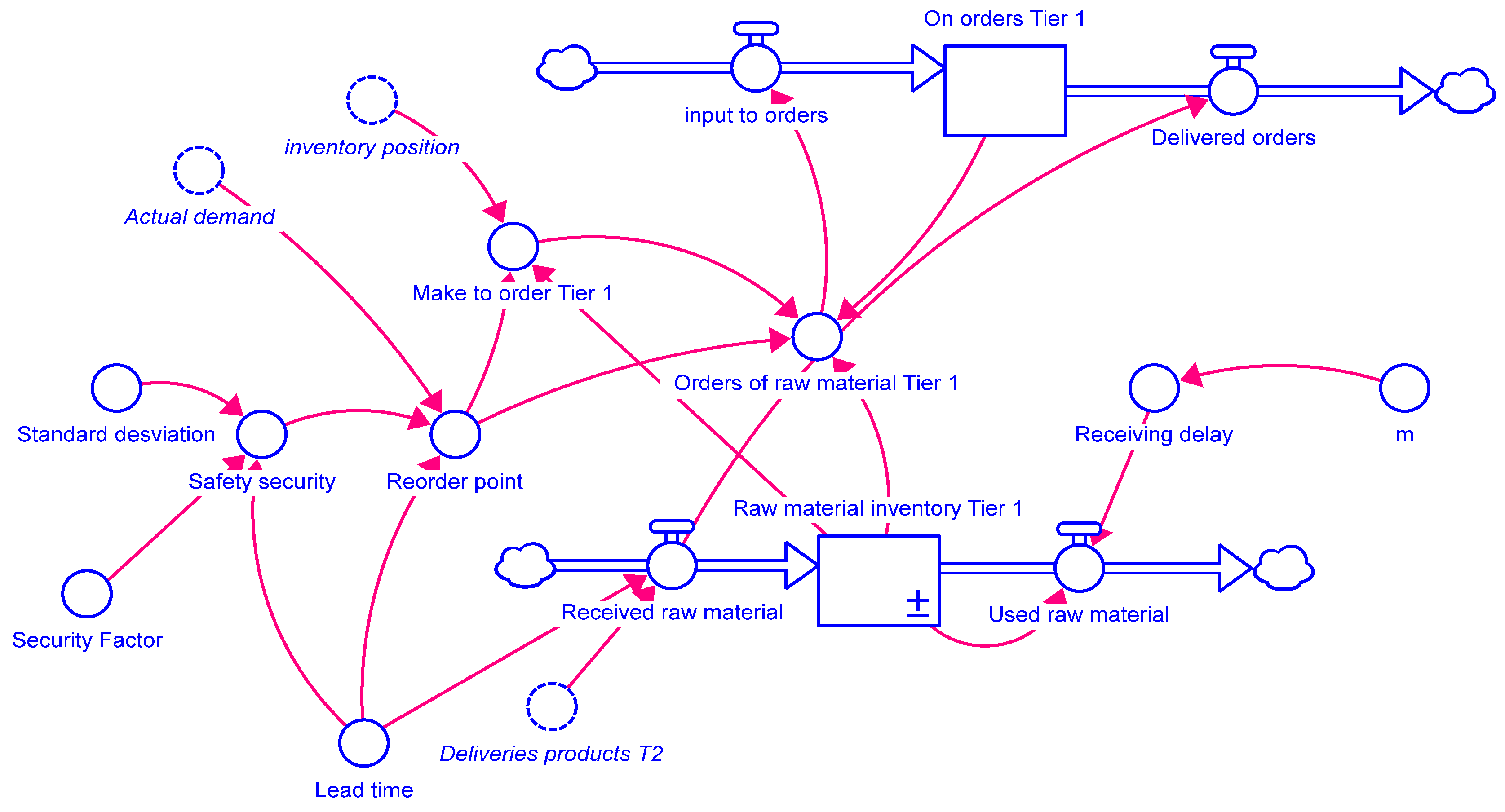
2.1. Dynamics System Modeling

This stage involves creating a system dynamics model that includes the variables that allow SC disruption to be modeled, considering the first two links, Tier 1 and Tier 2.

For this purpose, the flow, stock, and auxiliary variables were defined. The former is characterized by the quantities that enter the system, including their output, and are represented by arrows. The stock variables refer to the number of materials, for example, the quantity of inventory in the process, number of finished products available, and number of back orders pending delivery to the customer; squares represent them. Finally, the auxiliary variables are the parameters used to calculate the flow, and the circles represent the stock variables.

The automotive industry’s SC has three echelons: a Tier 1 supplier, Tier 2 supplier, and assembly plant (OEM). In this model, two echelons of the SC were integrated, and the flow of materials and disruptive capacity in the Tier 1 and Tier 2 links were also included. Flow and stock variables were used to develop mathematical models. These diagrams represent an approximation of the system by capturing the variables that influence it as a function of time. The validation was performed using dynamic hypotheses.

For the simulation of the model with various scenarios, Stella Architect Version 3.4.1 software was used in conjunction with 61 months of demand information, corresponding to the quantity of automotive-type materials obtained from real data in automotive companies for 2020 to 2023. The information for this study was collected through interviews with managers in demand planning, logistics, supply chain, and purchasing within the automotive industry. The data were captured in an Excel file in two columns: months and demand. These automotive industries are essential for accessing historical data to enrich the model. During data collection, we ensured the reliability of the data and adhered to privacy and confidentiality arrangements.

2.1.1. Definition of Equations and Parameters

In this section, we define the equations used for modeling, starting with the demand requested by the OEM assembler for the Tier 1 supplier. In addition, we include the demand for Tier 2 supplier, which corresponds to the raw material inventory of the Tier 1 supplier. This relationship is represented by Equation (1).

The raw material inventory is calculated using Equation (2), and the in-process inventory that helps to reduce production stoppages is obtained using Equation (3). The inventory of finished products for shipments is represented by Equation (4). On the other hand, the orders confirmed by the customer, where the demand and backorders with an adjustment time are included, are obtained using Equation (5). The products delivered to the customer are calculated using Equation (6), which determines whether the difference between the inventory of finished products and the completed orders is greater than zero; if this occurs, the complete orders are sent to the customer. The service level was calculated by dividing the products delivered to the customer by the completed orders using Equation (7).

On the other hand, backorders are considered in the supply chain echelons when there is no inventory capable of meeting the customer’s demand and are obtained using Equation (8). Equation (9) is used to add the entry of backorders in the last six months. Backorders delivered to the customer are fulfilled when demand is satisfied, and there is a sufficient inventory level, which is calculated using Equation (10). Using Equation (11), the quantity of material to be ordered from Tier 2 suppliers is obtained, whereas using Equation (12), the orders from Tier 1 suppliers are obtained.

The production rate considering the minimum value between the current capacity, the SC disruption, and the orders sent by the Tier 1 supplier to the Tier 2 supplier is calculated with Equation (13), to add the current capacity, Equation (14) is used. The raw material is the backlog of products delivered to the customer in two weeks obtained using Equation (15). The raw material used is established by dividing the raw material inventory by the backlog of orders and is calculated using Equation (16).

The reorder point is the minimum inventory that suppliers have to release their purchase order with a policy of periodic review and replenishment. It is obtained using Equation (17) to add the safety stock with a confidence level of 95%, and a standard deviation of the demand concerning the lead time and the time between orders is used in Equation (18). When the raw material inventory is less than the reorder point, the order is sent to a Tier 2 supplier. It is calculated using Equation (19) to aggregate the orders requested from Tier 2 suppliers. When the raw material inventory and Tier 1 supplier orders are less than the reorder point, a purchase requisition is released to the Tier 1 supplier, as shown in Equation (20). To add the Tier 1 supplier orders, Equation (21) is used, and it is important to consider the order entry to Tier 1 supplier with Equation (22), which corresponds to the orders delivered by Tier 1 supplier defined by Equation (23). Delayed receipts consider the disruptive risk plus the demand that is normally distributed with a mean and standard deviation (24), and disruptive risk is considered (25). The aforementioned equations are expressed as follows:

$$D_{kt}=D\ast \left(Normal\left(1,DV\right)\right)$$

(1)

where k, links in the supply chain, k = 3 is the assembler, k = 2 is the Tier 1 supplier, k = 3 is the Tier 2 supplier, t is the time in months from 1 to 61, D is the customer demand, DV is the demand variation from 0 < D < 1. Sanchez-Ramirez et al. [29] define the raw material inventory equation as follows:

$$IM{P}_t=IM{P}_{t0}+\underset{0}{\overset{t}{{\displaystyle \int }}}\left(RRM-URM\right)dt$$

(2)

where IMP is raw material inventory, URM is raw material orders received,$\mathrm{and} URM$ is raw material orders used. Olivares-Aguila and ElMaraghy [32] define the equation that describes the in-process inventory as follows:

$$WIP=WI{P}_{t0}+\underset{0}{\overset{t}{{\displaystyle \int }}}\left(PR-OS\right)dt$$

(3)

where WIP is work-in-process inventory, PR is production rate, and OS is ordered in shipments. Sanchez-Ramirez et al. [29] define the finished goods inventory equation as follows:

$$FGP=FG{P}_{t0}+\underset{0}{\overset{t}{{\displaystyle \int }}}\left(OS-DP\right)dt$$

(4)

where FGP is finished goods inventory; OS is ordered in shipments, and DP is products delivered to the customer. Olivares-Aguila and ElMaraghy [32] define the orders confirmed equation as follows:

$$OF=D_t+{\displaystyle \frac{ B{O}_t}{AT}}$$

(5)

where OF are the orders confirmed by the customer, D_t is the demand of the supply chain, AJ is the adjusted time, and BO_t is backorders. Olivares-Aguila and ElMaraghy [32] define the products delivered equation as follows:

$$DP=Min \left(OF, {\displaystyle \frac{FGP}{MTD}}\right)$$

(6)

where DP refers to the products delivered to the customer, FGI refers to the finished goods inventory, OF refers to the orders confirmed by the customer, and MTD refers to the minimum lead time. Olivares and ElMaraghy [32] define the service level equation as follows:

$$LS={\displaystyle \frac{DP}{OF}}$$

(7)

where LS is the service level, DP is the products delivered to the customer, and OF is the orders confirmed by the customer. Olivares-Aguila and ElMaraghy [32] define the backorders equation as follows:

$$BO=B{O}_{t0}+\underset{0}{\overset{t}{{\displaystyle \int }}}\left(IBO-BOD\right)dt$$

(8)

where BOs are back orders, IBOs are backorder entries, and BODs are back orders delivered to the customer. Olivares-Aguila and ElMaraghy [32] define the input back orders equation as follows:

$$IBO=IF \left(AD-DP\right) THEN (DP<AD) ELSE \left(0\right)$$

(9)

where AD is the actual customer demand, and DP is the products delivered to the customer.

Olivares-Aguila and ElMaraghy [32] define the backorders delivery to the customer equation as follows:

$$BOD=IF (IF {\displaystyle \frac{B{O}_{t }}{AT}} > 0 \mathrm{THEN} \mathrm{DP} = \mathrm{OF} \mathrm{ELSE} \text{DP-AD}) \mathrm{THEN} \mathrm{DP} > \mathrm{AD} \mathrm{ELSE} 0$$

(10)

where DP refers to the products delivered, OF refers to the orders confirmed by the customer, BO refers to the back orders, and AD refers to the actual customer demand. Bueno-Solano and Cedillo-Campos [28] define inventory position equation as follows:

$$IP=FGI-BO+WIP$$

(11)

where FGI is finished goods inventory, BO is backorders, and WIP is work-in-process inventory. Olivares-Aguila and ElMaraghy [32] describe the orders from Tier 1, which are calculated using the following equation:

$$OT1=IP$$

(12)

where IP is the lot size. Olivares-Aguila and ElMaraghy [32] define the production rate equation as follows:

$$PR=IF (RMI>=MIN\left(AC,OT1\right)) THEN \left(AC\right) ELSE \left(0\right)$$

(13)

where RMI is raw material inventory, AC is current production capacity, OT1 is Tier 1 orders Olivares-Aguila and ElMaraghy [32] define the current capacity equation as follows:

$$AC=TCT1-\left(TCT1\ast DCR\right)$$

(14)

where TCT1 is the total capacity of the Tier 1 supplier, and DCR is the capacity rate with disruption. Wilson [27] used the raw material in the following delayed equation:

$$RRM=DELAY \left(DP, LT\right)$$

(15)

where DP is the products delivered, and LT is the supplier’s delivery time. Olivares-Aguila and ElMaraghy [32] define the raw material used in the following equation:

$$URM=RMI/RD$$

(16)

where RMI is the raw material inventory, and RD is the order backlog. Ivanov et al. [41] define the reorder of point equation as follows:

$$\mathit{ROP}=\mathit{AD} \times (\mathit{LT}+\mathit{TO})+\mathit{SS}$$

(17)

where AD is the actual demand, LT is the lead time, TO is the time between two orders, and SS is the safety stock. Ivanov et al. [41] define safety stock through the following equation:

$$\mathit{SS}=\mathit{SF} \times \mathit{SD} \times \sqrt{\mathit{LT}+\mathit{TO}}$$

(18)

where SF is the safety factor, assuming a 95% confidence level with a normal distribution equal to 1.65, SD is the standard deviation of the demand, LT is the lead time, and TO is the time between orders. The deviation concerning lead time and time between orders is determined. Bala et al. [42] define make to order equation as follows:

$$\mathit{MO}=\mathit{IF} \left(\mathit{RMI} < \mathit{ROP}\right) \mathit{THEN} \left(\mathit{IP}\right) \mathit{ELSE} \left(0\right)$$

(19)

where OTMT2 is the raw material order, RMI is the raw material inventory, ROP is the reorder point with a periodic review policy, and IP is the lot size convenient for ordering from the supplier. Olivares-Aguila and ElMaraghy [32] define the purchase requisition to Tier 2 supplier equation as follows:

$$\mathit{OTMT}2=\mathit{IF} \left( \left(\mathit{RMI}+\mathit{OT}1\right) < \mathit{ROP}\right) \mathit{THEN} \left(\mathit{MO}\right) \mathit{ELSE} \left(0\right)$$

(20)

where RMI is the raw material inventory, OT1 is the Tier 1 supplier orders, ROP is the reorder point, and MO is the order shipment to the Tier 2 supplier. Olivares-Aguila and ElMaraghy [32] define the orders entry to Tier 1 supplier equation as follows:

$${\mathit{OOT}1=\mathit{OOT}1}_{t0}+\underset{0}{\overset{t}{{\displaystyle \int }}}\left(\mathit{IO} - \mathit{DO}\right)\mathit{dt}$$

(21)

where IO is the orders received by the Tier 1 supplier, and DO is the orders delivered by the Tier 1 supplier. Olivares-Aguila and ElMaraghy [32] define the order entry to Tier 1 supplier equation as follows:

$$\mathit{IO}=\mathit{OMT}2$$

(22)

where OMT2 are raw material orders to Tier 2 suppliers. Olivares-Aguila and ElMaraghy [32] define the orders delivered by Tier 1 through the following equation:

$$\mathit{DO}=\mathit{RRM}$$

(23)

where RRM is the raw material received. Bala et al. [42] define receiving delay equation as follows:

$$\mathit{RD}=0.5+0.10m+N(\mathit{DM},\mathit{SD})$$

(24)

where RD is the delayed receipts, N is the demand with a normal distribution, DM is the average demand, and SD is the standard deviation of the demand. Bala et al. [42] define the disruptive risk equation as follows:

$$\mathrm{m}=\left(\mathrm{RAMP}\right(0.7,110,150)/8)+0.9 - \mathrm{STEP}(3.3,150)$$

(25)

where m is the disruptive risk.

2.1.2. Integrating Information into Stella

To identify demand information, interviews were conducted with managers of Tier 1 and Tier 2 suppliers who supplied vehicle components to OEMs. The questions include (a) the amount of initial inventory, (b) the lead time, and (c) the safety inventory to feed the equations under the initial conditions of Section 2.1.1.

The model is based on a Tier 1 supplier company dedicated to manufacturing gasoline tanks. This company has a disruptive capacity of 2500 gasoline tanks for a vehicle assembly company (OEM) Sedan type, representing 4% of the monthly production.

Based on the above, the following are modeled in the Stella Architect software: (a) behavior demand variability, (b) level of raw material inventory both in process and finished product, (c) orders sent to the customer and Tier 2 supplier, (d) backorders, and (e) production capacity with disruption. Response variables such as customer service level and disruption detection were also included.

2.1.3. Evaluating Causal Model of Disruption

To evaluate disruption, the disruptive capacity rate is incorporated with values of 0 < X < 1, where zero indicates no disruption, 0.25 indicates one technical strike in the company due to delay of materials and equipment failures, 0.50 indicates material shortage due to the supplier, and 1.0 indicates severe disruption equivalent to 15 days of suspension of operations. The reorder point is based on an average demand of 6797 gasoline tanks, with a standard deviation of 1638 gasoline tanks with security factor of 95% which estimates the probability of avoiding a stockout of raw materials in the automotive industry. The initial stock is 3500 gasoline tank, corresponding to two weeks of inventory. The lead time is two weeks, and the time between orders from Tier 2 suppliers is of one week.

2.1.4. Interpretation of the Performance of Results

To interpret performance, we first consider the production rate influenced by the raw material inventory, disruptive capacity, and orders sent by the Tier 1 supplier to the customer. These orders correspond to many sizes that are convenient to request from the raw material supplier.

In addition, shipments are delayed by one week owing to transportation risks, which decreases the inventory of products delivered. Consequently, orders delivered to customers have also decreased. However, the level of service is inversely proportional between orders delivered to the customer and those confirmed by the customer. Receiving delays is a disruptive risk, raised as a cascade of cancelations of orders requested by the customer and influencing the shortage of materials by suppliers globally, resulting in a lower level of service.

2.2. Artificial Neural Networks Based on the Detection of Disruptions

The literature reports various solutions based on artificial neural networks (ANN) to analyze disruptions in supply chains. For instance, Liu et al. [43] proposed a model design using gray neural networks primarily aimed at optimizing inventory and production following disruption. Similarly, Bodendorf et al. [44] combined causal inference and deep learning to analyze and predict supply chain disruptions, and Tang et al. [45] introduced a monitoring model that automatically identified industrial chain disruption events using deep learning technology. This study aims to detect disruptions, and a new network design methodology is proposed tailored to the disruption context.

2.2.1. Data Monitoring

The proposed network monitors relevant data for disruption detection and constantly feeds such data to the neural network. Several industrial data sources can be used to detect disruptions in the supply chain early. These sources can be classified into two main categories: internal and external sources.

The internal sources are historical data from risk management processes and internal communication. The latter can be established by implementing communication channels between all departments involved in the supply chain. External sources include industry news and reports that can identify potential risks by learning from events occurring in other companies, customers, and suppliers. These data can provide information about potential problems in the supply chain.

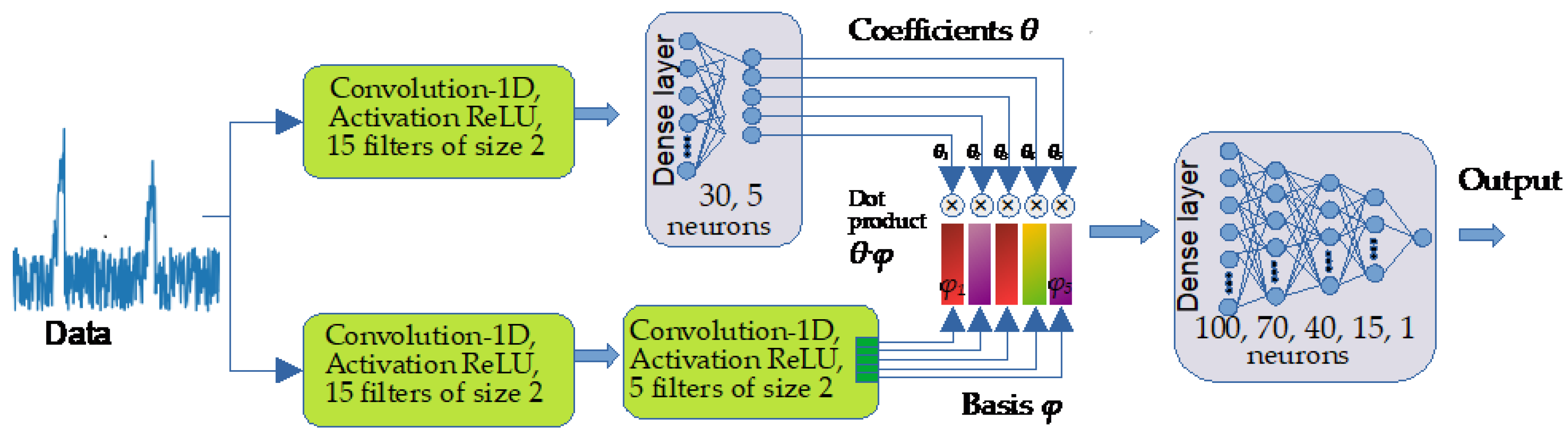
2.2.2. Deep Learning Architecture for Disruption Detection

The early detection of disruptions is important because it allows for timely response and reduced impact [45,46]. Here, we propose a neural network to help evaluate disruption risks in supply chains.

The proposed neural network architecture is based on monitoring time-series data correlated with disruptions such as operational events and environmental phenomena that could impact a company, its suppliers, customers, and transportation links (Sheffi [47]).

For the design of the proposed architecture, we base the architecture on generalized nonlinear AR models [48,49]; however, we also aim for the architecture to stay simple and generic and not rely on manual feature engineering. The classic AR model for a time series x is as follows.

$$x_{t+1}=a_{t-1}{x}_{t-1}+\dots +a_{t-k}{x}_{t-k}+z_{t+1}$$

(26)

where there are coefficients or model parameters, is the order of the model, and is the white noise process. The generalization of Model (1) is as follows:

$$x_{t+1}={\mathsf{\theta }}_{t-1}{\phi }_{t-1}+\dots +{\mathsf{\theta }}_{t-k}{\phi }_{t-k}$$

(27)

In this case, θs are coefficients, and φs are tensors based on past data ($x_{t-1},\dots ,x_{t-k})$. Our approach for designing a deep learning architecture consists of finding coefficients, θ, and tensors φ, based on historical data. To achieve this, we employed a parallel architecture with two vias, as shown in Figure 2. One via extracts the coefficients, θ, from the data, while the other extracts the tensor representations, φ, which we refer to as the basis tensors. Thus, we obtain a richer representation of the series elements in terms of basis tensors. Based on this representation and the MLP layer, the classifier stage of the model estimates the probability that the term is part of a disruption.

2.2.3. Model Implementation

The implementation details are as follows. The input to the proposed architecture was a time series. This series included historical data on supplier performance, transportation delays, inventory levels, economic indicators, weather patterns, geopolitical events, and other relevant variables. The network structure is illustrated in Figure 2.

For this case, a value for $k=5$ in Equation (26) was determined empirically by testing various values and balancing precision with computational cost. Thus, Equation (27) consists of five terms: ${\mathsf{\theta }}_1{\phi }_1+{\mathsf{\theta }}_2{\phi }_2+{\mathsf{\theta }}_3{\phi }_3+{\mathsf{\theta }}_4{\phi }_4+{\mathsf{\theta }}_5{\phi }_5$. The coefficients $\mathsf{\theta }$ are calculated through the first via, which begins with a convolutional layer consisting of 15 filters of size 2, followed by two dense layers with 30 and 5 neurons, respectively. All the layers used ReLU activation functions. The neurons in the final dense layer output the ${\mathsf{\theta }}_{1:5}$ values.

The second via computes the ${\phi }_{1:5}$ basis tensors. This starts with a convolutional layer of 15 filters of size 2, followed by another convolutional layer with 5 filters (k = 5) of size 2. The feature maps produced by this final layer represent the basic functions ${\phi }_{1:5}$. To obtain the new representation, each feature map φ_I is multiplied by its corresponding coefficient θi, where I goes from 1 to 5, and the results are summed. This combined representation is then fed into the classification stage, a dense network with layers of 100, 70, 40, 15, and 1 neuron, respectively. The first four layers used a rectified linear unit activation function, and the last neuron used a sigmoid function. Finally, the output neuron determines whether a disruption is present in the input data, with a value of one indicating disruption and zero indicating no disruption. The network was trained using a cross-entropy loss function with an adaptive moment optimizer (Adam) to improve the learning efficiency of the model.

The system dynamics model generated data and simulated several disruptions to train the neural network. The proposed neural network architecture learns to make predictions by minimizing a loss function that measures the difference between predicted and actual labels in the training data.

3. Results

Here, we present the implementations and tests of the system dynamics model and the results obtained in the proposed architecture for detecting disruptions by integrating system dynamics and artificial intelligence.

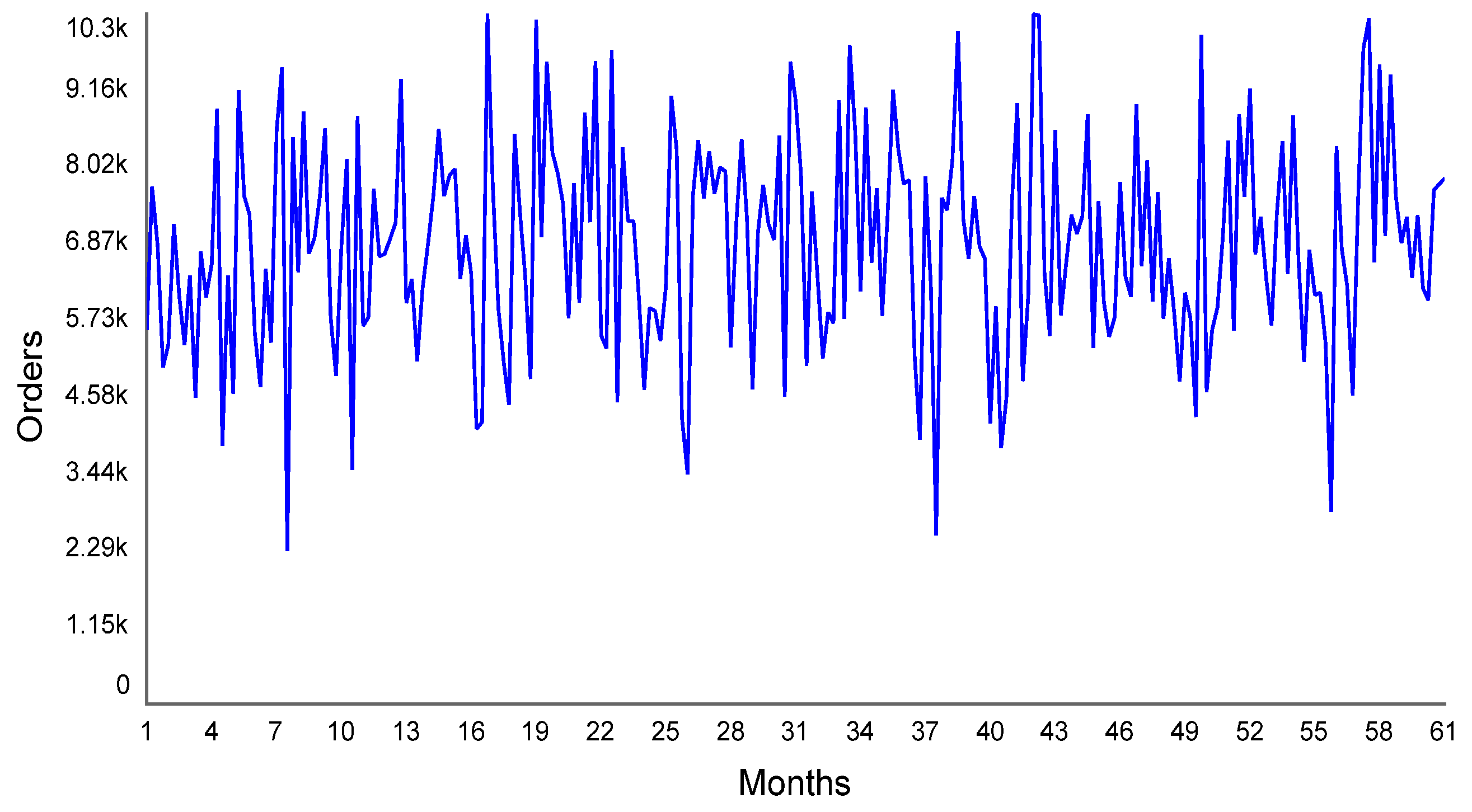
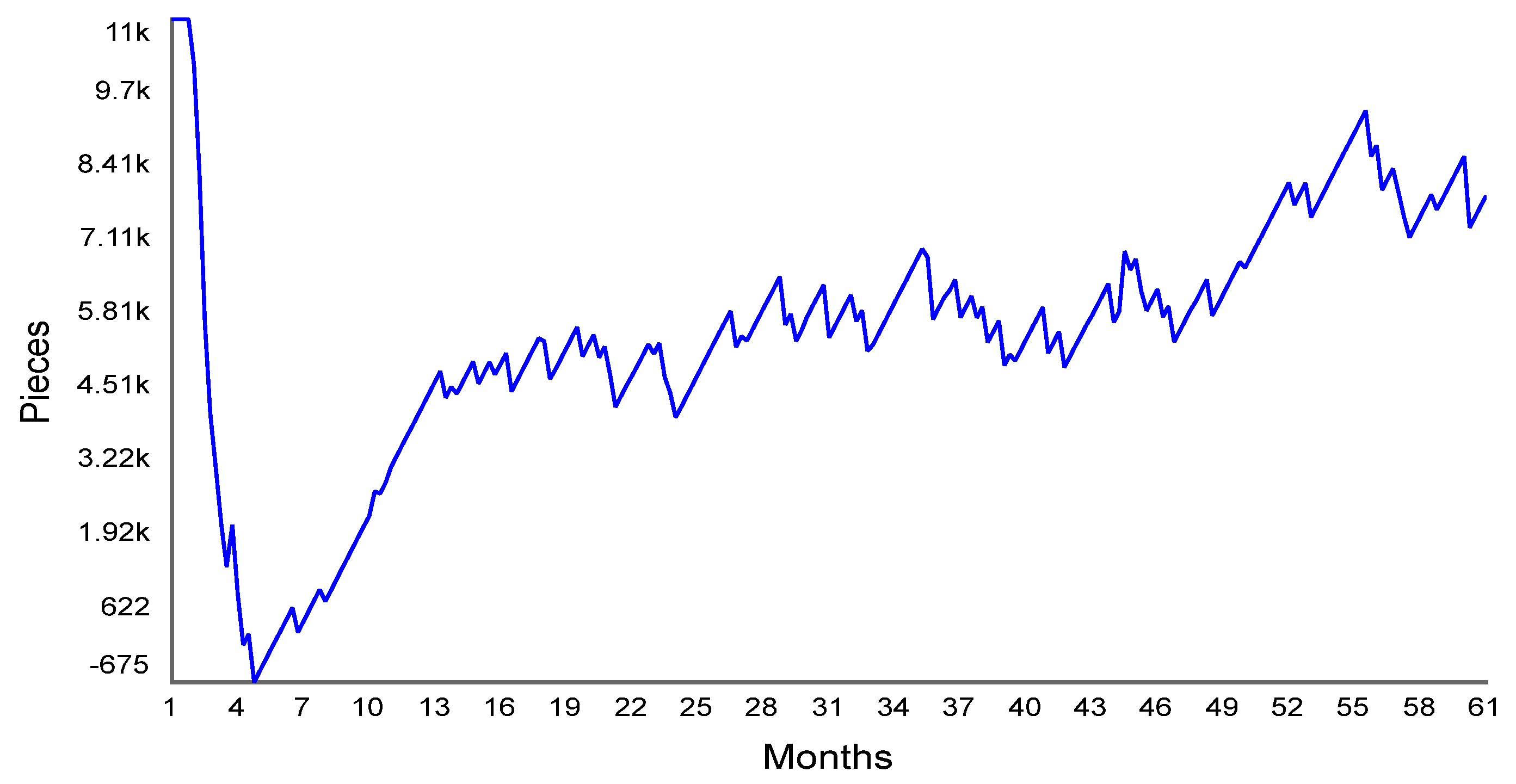
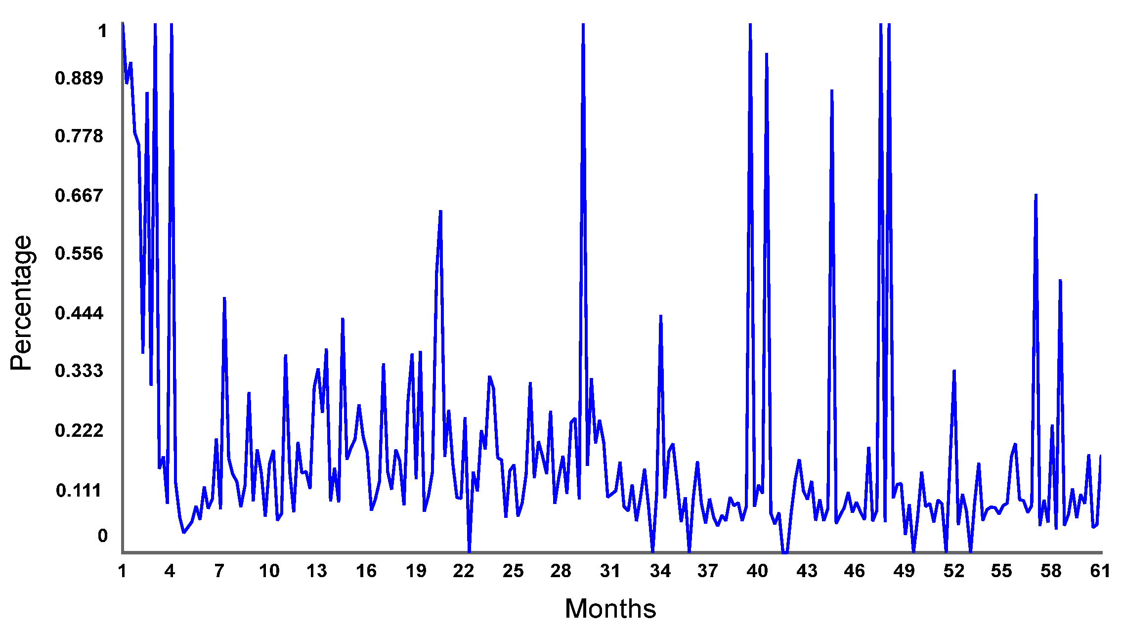
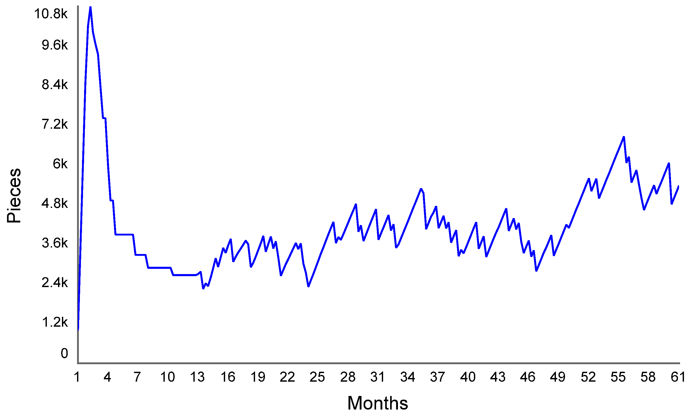
3.1. System Dynamics Model Results

The results of the model are shown in two parts: the first in Figure 3 and the second in Figure 4. Figure 3 shows that the Tier 1 supplier requests raw materials according to the demand requested by its customer (the assembly plant). The policy established by the Tier 1 supplier is to verify the level of inventory that it has in its warehouse of materials, corresponding to the number of orders received, and that presents a delay of two weeks by the Tier 2 supplier caused by a shortage of material. Supplier Tier 1 sends the material order to supplier Tier 2, considering the reorder point with a replenishment policy.

The reorder point was calculated using the average demand of 6760 tanks of gasoline that comes from the assembler for a delivery time of one week when they are domestic suppliers; in the case of suppliers that are located internationally, it is three months plus the safety stock that has a safety factor of 95% reliability, which indicates that the Tier 2 supplier has an inventory level to cover the order requested by the Tier 1 supplier, avoiding the shortage of material and a standard deviation of 1637 tanks of gasoline. The Tier 1 supplier is established to manufacture according to the order received from the assembler when the inventory of raw materials in its warehouse is less than the reorder point. Supplier Tier 1 also has orders scheduled for delivery, considering the income from purchase orders sent by the assembler minus the orders delivered to the customer.

It is important to note that to achieve the model, the demand was obtained from a database, in Excel with xlsl format, of 61 months with a variability from −0.5 < D < 1. The modeling of the dynamic system to detect disruption in the supply chain in this automotive industry case considered 10 scenarios, as shown in

Table 2. Disruption scenarios in the supply chain automotive industry.

Scenarios	Demand Variation	Disrupted Capacity Rate	Lead Time	Delay
1	0	0	0.25	0.25
2	0.2	0.5	0.5	0.5
3	0.50	0.50	0.50	0.50
4	−0.20	0.50	0.50	0.50
5	−0.50	0.50	0.50	0.50
6	0.2	0.7	1	1
7	0.50	0.7	1	1
8	0.7	0.7	1	1
9	−0.2	0.7	1	1
10	−0.5	0.7	1	1

. In the proposed model, there are scenarios without disruption and with disruption. Scenario one is without disruption, with a stable demand, a lead time of one week, and a delay of one week. Scenarios two and three, with an increase in customer demand from 20% to 50% and a 50% disruption, resulted in a production delay of two weeks due to the shortage of materials from the Tier 1 supplier. The results obtained in scenarios four and five show that customer demand decreased by 50% because of the global shortage of materials from suppliers. For scenarios six and seven, customer demand increased by 50% with a severe disruption of 0.7, indicating the suspension of operations in the entire automotive supply chain for four weeks caused by the shortage of materials from the Tier 2 supplier.

Scenario eight shows that customer demand increased by 70%, and with a severe disruption of 0.7, suppliers began to decrease their material inventory owing to the suspension of operations. Therefore, in scenarios 9 and 10, customer demand decreased by 70% owing to increased lead times of four weeks from suppliers located in Mexico and 16 weeks from international suppliers.

Figure 4 shows the automotive supply chain disruption that starts with material inventory in the warehouse. Then, the production order is released when the raw material inventory is greater than or equal to the minimum capacity between the current capacity and orders shipped to the customer by the Tier 1 supplier. Current capacity is determined by the Tier 1 supplier’s total capacity multiplied by the disruptive capacity of 0 < DCR < 1. Tier 1 orders equal the lot size determined by the finished goods inventory plus backorders minus the in-process inventory. Orders ready to ship are delayed by a maximum of four weeks, which is equivalent to one month of production. The initial inventory of finished gasoline (1800) was equivalent to one week. The delivery policy of gasoline tanks to Toyota is that the inventory of finished products minus the completed orders, including the backlog of orders, must be greater than zero. Consequently, completed orders are delivered. The service level is calculated as the quantity of orders delivered to the customer between completed orders and customer demand plus back orders. Backorders include the entry of backorders when the products delivered to the customer are less than the demand, minus the backorders delivered to the customer.

Figure 5 shows the results of the analysis of order reception behavior, considering a two-week delay from the Tier 2 supplier from April 2020 to November of the same year and a 75% decrease in gasoline tank production. This is due to supply chain disruption caused by the global shortage of components during the pandemic.

On the other hand, the behavior of the orders delivered to the client by the Tier 1 supplier was also analyzed; the results are shown in Figure 6, where it is observed that from January to March 2020, orders were delivered completed according to the requirements requested by the client. However, in April of the same year, when the automotive supply chain suspended operations due to COVID-19, orders delivered to customers decreased drastically. Subsequently, the automotive industry began to recover when the demand for components increased by 80%, from 4500 to 8300 gasoline tanks in three years, referring to the demand for vehicles.

In addition, the Tier 1 supplier’s service-level behavior was analyzed, as shown in Figure 7. It was observed that it decreased from 80% requested by the customer before the pandemic to 65% due to the decrease in demand from 10,369 to 4102 from April 2020 to August 2020. However, delivery times by Tier 1 suppliers to their customers continue to increase owing to component shortages.

Finally, the Tier 1 supplier’s finished goods inventory level was analyzed, as shown in Figure 8. The results indicate an impact reduction of 66% in the finished goods inventory level due to the suspension of operations of the automotive industry in Mexico because of COVID-19 during the first half of 2020. Subsequently, the inventory level was increased by 30%, representing a one-week safety stock that helps the Tier 1 supplier supply customer demand. However, if the customer increases demand by 50%, Tier 1 supplier is delayed by one week in delivering the order because of Tier 2 supplier’s shortage of materials.

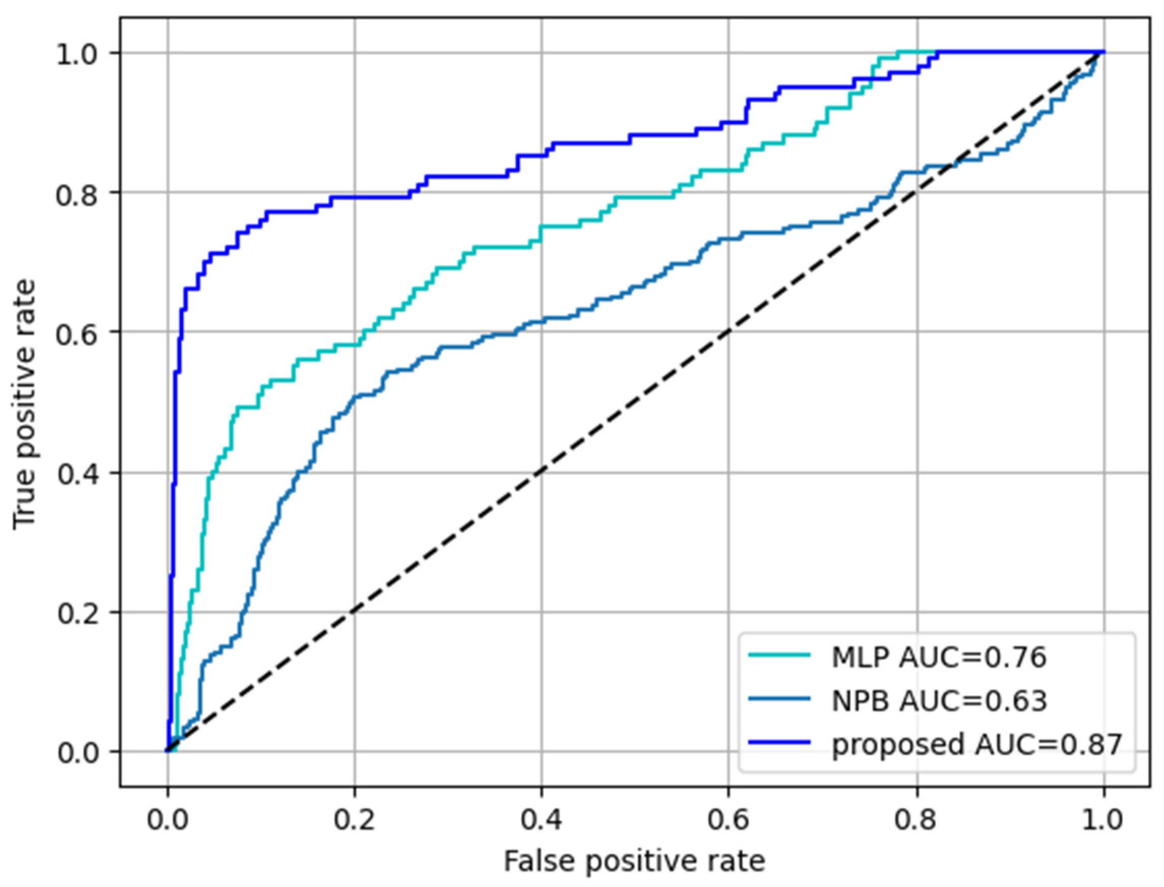
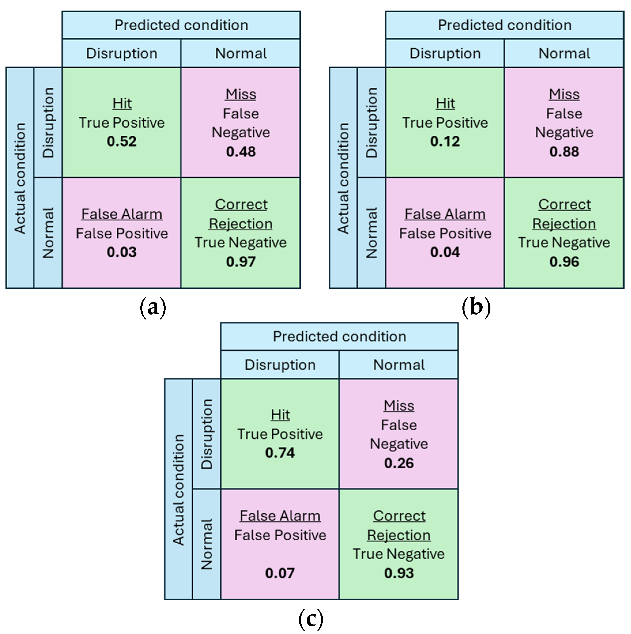
3.2. Network Evaluation in the Model

The performance of the proposed model is presented herein. The idea is to detect a disruption before it is evident using data on operating events and environmental phenomena that could impact the company. The receiving delay was used as the input for the proposed method in the experiments. For comparison, two other methods were used: a neural network estimator based on, Refs. [45,47] for disruption detection and consisting of a multi-layer perceptron (MLP) with four hidden layers and 75 neurons in each hidden layer. And a Neyman-Pearson (NPB) based detector that assumes Gaussian distribution [44,46].

Disruption scenarios were generated by using a system dynamics model to train and test the models no pre-processing was made. The data were divided into segments of 15 samples. If a segment contained at least one sample associated with a disruption, it was labeled as a disruption; otherwise, it was classified as a normal segment. A total of 1500 samples were simulated, incorporating periods of normality and random disruptions. The task of the algorithms is to classify each segment as either part of a disruption or an abnormal event. A training set with 80% of the data were used, and 20% was used for testing.

Figure 9 shows the resulting Receiver Operating Characteristic (ROC) curves of the proposed model and other comparison methods. These curves show the tradeoff between the true- and false-positive rates at various threshold settings. This helps assess how well a model distinguishes between disruption and normal scenarios. In the context of ROC analysis, the Area Under the Curve (AUC) quantifies the overall performance, with higher AUC values indicating better model performance. For comparison, two other methods were used: a neural network estimator based on [44,50] for disruption detection and consisting of a multi-layer perceptron (MLP) with four hidden layers and 75 neurons in each hidden layer. And a Neyman-Pearson-based (NPB) detector that assumes Gaussian distribution for the product [44,46]. Figure 9 shows the ROC curves of the proposed network and the other methods used for comparison. As can be observed, the AUC is notably more significant for the proposed network. An AUC comparison using the DeLong test, DeLong et al. [51] was conducted to statistically evaluate the differences between the curves. The results are as follows. For MLP vs. NPB (AUC = 0.76 and 0.63, respectively), a Z-score of 5.1042 and a p-value of 0.00001 were obtained, confirming a statistically significant difference, with MLP clearly outperforming NPB. For MLP vs. the proposed network (AUC = 0.76 and 0.87, respectively), a Z-score of −2.5910 and a p-value of 0.0096 indicate that the proposed network outperforms MLP. For NPB vs. the proposed network (AUC = 0.63 and 0.87, respectively), a Z-score of −18.0136 and a p-value of 0.00001 confirm a statistically significant difference, demonstrating that the proposed network is superior to NPB.

Figure 10 shows the confusion matrices for the different methods, which has fewer false positives than the other methods, the proposed approach generates fewer alerts that turn out to be negligible. Thus, by offering reduced wasted time, analysts can focus on real issues requiring attention instead of investigating non-existent disruptions. In addition, our proposed method attains fewer false negatives, meaning it misses fewer actual disruptions, and corrective actions can be taken to minimize downtime, prevent product defects, and mitigate security risks.

Table 3. Summary of precision, recall, and F1 score metrics.

Class	Method	Precision	Recall	F1-Score
	MLP	0.92	0.97	0.94
Normal	NP	0.72	0.96	0.82
	Proposed	0.95	0.93	0.94
	MLP	0.76	0.52	0.62
Disruption	NP	0.57	0.12	0.20
	Proposed	0.65	0.74	0.69

shows the performance of the methods for precision, recall, and F1-score metrics.

4. Discussion

The simulation was carried out for five years with initial parameters to determine a starting scenario that helps simulate the detection time of the disruption. The objective was to detect the disruption in the supply chain in the automotive industry in Tier 1 suppliers using a dynamic model, where the behavior of the system that influenced the variables receiving delay and service level under different conditions was analyzed, for example, with scenario five according to, Ghadge et al. [40] demonstrated with a decreased demand of 50%, impacted the increase in risk to suppliers where the disruptive capacity was increased to 0.5 which influences the lead time of 0.5 months plus the delay of materials of 0.5 months.

When evaluating the disruption in the supply chain of the automotive industry during the pandemic in scenario 5 with a decrease in demand of 50% and a disruptive capacity rate of 0.5, caused by the shortage cancelations of orders requested by the customer Tier 2 supplier for two weeks. The inventory level of finished products decreased by 75%, which influenced the increase in Therefore, it was determined that the inventory level of finished products decreased by 75%, which influenced the increase in cancelations of orders requested by the customer. As a result, operations in the supply chain were suspended because of the shortage of materials, which favored the increase in backorders delivered to the customer. As a result, the service level decreased, affecting the performance level of Tier 1 supplier, which fulfilled customer demand by 68%. Compared with, Lai et al. [25], which used a safety stock coefficient of 0.45, a service level of 53.53% was obtained. In this scenario, the service level favors the domino effect over five years. This scenario helps supply chain managers make decisions in advance; for example, increasing the inventory level to three weeks with an increase in the costs of keeping inventory in stock.

This model has different assumptions such as the downstream actual demand that follows a normal distribution with a mean and standard deviation, variable lead time from one week to four-week, security factor of 95% that indicates a lack of stock will not delay deliveries products with risk of a stockout of 5% with an inventory control policy periodic review where include variable time between two orders. That impact in supply chain performance such as finished goods inventory, service level, The disrupted capacity is long term and depend on the disruptive risk. The constraints of the model exclude the total cost supply chain disruption, the datasets are of 60 months. Because its complex for automotives industries provides your information about historical demand of ten years could impact the accuracy predictions. The model has two echelons, supplier Tier 2 and supplier Tier 1 in the supply chain automotive industry and simulate only gasoline tanks. The simulation model could be approximate with respect to real world.

For the proposed deep learning architecture for disruption detection, the ROC plotted in Figure 8 shows that the AUC for the proposed network was 0.87, which is the highest among the evaluated models. MLP achieved an AUC of 0.76, whereas the NP model showed a significantly lower AUC of 0.63. These results indicate that the proposed model exhibits more discriminative power, distinguishing between disruption events and normal cases more reliably than other models.

Table 3 shows that the MLP method had moderate precision in detecting disruptions, correctly identifying 76% of the predicted disruptions. However, it missed many disruptions, detecting only 52% (Recall = 0.52) of the actual disruptions. An F1-score of 0.62 indicates that the MLP method is acceptable for detecting disruptions but struggles with recall. In the case of the NPB method, its precision is quite low, with only 57% of its disruption predictions being correct, achieving equally low scores for recall and the F1-score.

On the other hand, the proposed method has lower precision than MLP but is still more reliable than NPB (65% precision). However, it achieves higher recall compared to the other methods, detecting 74% of the disruptions, which is significantly higher than that of MLP. In addition, the F1-score of 0.69 is the highest for the disruption class, indicates that the proposed method best detects disruptions in a balanced way between precision and recall. Thus, the proposed method offers the best overall solution for handling disruptions. While MLP is strong in detecting normal instances, its recall for disruption is limited, and NP is not competitive overall because of its low recall and poor F1-scores. The proposed method provides a good compromise between detecting normal and disruption cases, with better overall F1 scores across both classes.

Traditional disruption detection models, such as rule-based systems and statistical thresholding methods, rely heavily on predefined conditions and historical data patterns. While these methods are frequently simpler, they often struggle with adapting to complex, evolving disruptions and have limited generalization capabilities when faced with unseen events.

Machine learning-based models, such as MLP and NP, improve upon traditional approaches by learning from data and detecting disruptions more flexibly. However, as observed in the results, MLP struggles with recall, missing a significant number of disruptions, while the NP model performs poorly overall due to its low precision and recall. These limitations stem from the fact that traditional models and basic machine learning approaches often do not effectively capture temporal dependencies or account for diverse industrial data sources.

Detecting the disruption early in Tier 1 suppliers implies reducing the number of orders shipped to their suppliers internationally. This helps maintain a safe stock of finished products equivalent to two weeks of production, reduces the cost per order, and shortens the lead time to increase customer service.

The implementation of the proposed deep neural network in industrial applications presents several challenges. Industrial data sources are heterogeneous and often noisy, requiring efficient integration and preprocessing. Additionally, real-time disruption detection demands low-latency inference. Another critical issue is data imbalance, as disruptions are rare events, making it harder for the model to generalize. Lastly, evolving supply chain risks necessitate a model that can adapt dynamically without extensive retraining. To address these challenges, the proposed architecture integrates convolutional layers to extract key statistical features and tensor representations, improving robustness against noise and variability. Its computational efficiency can be enhanced through optimization techniques such as pruning and fog computing integration. To handle data imbalance, strategies like data augmentation and anomaly detection can be employed. Additionally, continuous learning mechanisms, including transfer learning and online adaptation, enable the model to remain relevant as supply chain conditions evolve. These solutions ensure that the architecture remains scalable, interpretable, and effective for real-world industrial disruption detection. The domino effect in the supply chain and with respect to risk management is an event that begins with reaction effects and ends in adverse chain events, affecting all companies within it. Recently, research has integrated new ways of evaluating this effect, mainly due to the strength in the use of computational analysis and the advance in neural network algorithms. In this case, by incorporating simulation and machine learning algorithms, it is a cutting-edge way of assessing risk, thus improving its visualization and accuracy compared to traditional methods.

This goes beyond a simple analysis, as it encourages the creation of early response strategies to disruptions, in order to also optimize the resources available to the company to manufacture. In the industrial field, managers could predict the likely ripple effects in some parts of their process to avoid delays in their product deliveries to their customers and reduce costs associated with it. With the appearance of recent natural disasters or health risks, such as the pandemic, this would allow anticipating the acquisition of raw materials. This model was made from data from the automotive sector, but it can be applied to any industrial field since the algorithm is versatile and adaptable to the data with which its learning is trained. Companies can integrate this model in a simple way, since they have information from historical data such as costs, inventory quantity, delivery time, and demand. These are used so that the proposed model achieves a retraining and the prediction is achieved.

5. Conclusions

This study successfully integrated a system dynamics model with a deep learning architecture to detect supply chain disruptions in the automotive industry, specifically for Tier 1 suppliers. The disruptions were caused by material shortages at Tier 2 suppliers over a four-week period from April to November 2020. This affected the decrease in demand by 50%, which reduced the level of service in the supply chain.

By integrating the dynamic model with machine learning, it was possible to evaluate the impact of the disruption by observing the reduction in the number of orders received by the Tier 1 supplier, the decrease in finished product inventory levels, and the increase in the backlog of orders, all of which influenced the decline in the level of service owing to material shortages during the pandemic. This also led to longer delivery times by the Tier 2 supplier, who assumed greater risk within the supply chain.

By modeling the real demand of an automotive company producing gasoline tanks with a normal distribution from January 2019 to January 2024, a reduction in customer demand between 20% and 50%, combined with a severe disruption factor of 0.7, amplifies the ripple effect throughout the supply chain, mainly affecting Tier 2 suppliers, who must adjust their master production schedules and incur higher costs to meet customer demand.

These scenarios allow automotive managers to understand the importance of detecting disruptions in the supply chain to prevent material shortages. Maintaining a two-week finished goods inventory level can reduce lead times to customers and mitigate the domino effect. as Additionally, these insights support decision-making by optimizing the number of orders shipped to their suppliers internationally and implementing supplier-managed inventory to improve responsiveness and share risk between both parties.

The dynamic model based on deep learning reveals that the domino effect delays the receipt of orders due to a decrease in the supplier’s raw material inventory. Additionally, global raw material shortages increase costs, further reduce the performance of the supply chain in terms of service level and customer satisfaction and, as a result, reduce the customer’s profitability. This model also detects disruptions in the supply chain and helps predict the risk of a domino effect in subsequent years by maintaining an optimal safety stock of materials and finished products to improve customer satisfaction.

This model has practical implications, although obtaining historical data for five years can be complex, which may impact the accuracy of predictions affecting key performance indicators such as initial security stock, cost of raw materials, delivery time, and service levels. However, the algorithm can be applied to any industry field.

For future research, we will consider extending the amount of historical data concerning demand and factors related to transportation and risks, incorporating the domino effect. Finally, in the short term, we aim to extend the supply chain disruption detection model for Tier 2 suppliers by integrating machine learning models into the dynamic system to predict disruption in future years. The contribution to the literature integrates new methods for evaluating the ripple effect that affects the companies within the supply chain. In this case, we incorporate a dynamic simulation model and machine learning algorithms to improve the visualization and accuracy of predictions compared to traditional methods. Practically, this approach helps managers make informed decisions, such as increasing raw material inventory levels to avoid stockouts.

References

1. Remko, V.H. Research opportunities for a more resilient post-COVID-19 supply chain-closing the gap between research findings and industry practice. Int. J. Oper. Prod. Manag. 2020, 40, 341–355. [Google Scholar] [CrossRef]
2. Ivanov, D.; Dolgui, A. OR-methodsfor coping with the ripple effect in supply chains during COVID-19 pandemic:Managerial insights and research implications. Int. J. Prod. Econ. 2021, 232, 107921. [Google Scholar] [CrossRef] [PubMed]
3. Ivanov, D. Predicting the impacts of epidemic outbreaks on global supply chains: A simulation-based analysis on the coronavirus outbreak (COVID-19/SARS-CoV-2) case. Transp. Res. Part E Logist. Transp. Rev. 2020, 136, 101922. [Google Scholar] [CrossRef] [PubMed]
4. Cannella, S.; Ponte, B.; Dominguez, R.; Framinan, J.M. Proportional order-up to policies for closed-loop supply chain: The dynamic effects of inventory controllers. Int. J. Prod. Resc. 2021, 59, 3323–3337. [Google Scholar] [CrossRef]
5. Matsuo, H. Implications of the Tohoku earthquake for Toyo ota׳s coordination mechanism: Supply chain disruption of automotive semiconductors. Int. J. Prod. Econ. 2015, 161, 217–227. [Google Scholar] [CrossRef]
6. Ivanov, D.; Tsipoulanidis, A.; Schönberger, J. Supply Chain Risk Management and Resilienc. In Global Supply Chain and Operations Management: A Decision-Oriented Introduction to the Creation of Value; Ivanov, D., Tsipoulanidis, A., Schönberger, J., Eds.; Springer International Publishing: Cham, Switzerland, 2021; pp. 485–520. [Google Scholar]
7. Mashud, A.H.M.; Hasan, M.R.; Daryanto, Y.; Wee, H.-M. A resilient hybrid payment supply chain inventory model for post COVID-19 recovery. Comput. Ind. Eng. 2021, 157, 107249. [Google Scholar] [CrossRef]
8. Saleheen, F.; Habib, M.M. Global Supply Chain Disruption Management Post COVID-19. Am. J. Ind. Bus. Manag. 2022, 12, 376–389. [Google Scholar] [CrossRef]
9. Kinra, A.; Ivanov, D.; Das, A.; Dolgui, A. Ripple effect quantification by supplier risk exposure assessment. Int. J. Prod. Res. 2019, 58, 5559–5578. [Google Scholar] [CrossRef]
10. Zhong, J.; Jia, F. Supply chain risk transmition monitoring based on graphic evaluation and review technique. Heliyon 2025, 11, e41462. [Google Scholar] [CrossRef]
11. Xu, X.; Tatge, L.; Xu, X.; Lio, Y. Block chain application in the supply chain management in German automotive industry. Prod. Plan. Con. 2022, 56, 917–931. [Google Scholar] [CrossRef]
12. Ivanov, D.; Sokolov, B.; Solovyeva, I.; Dolgui, A.; Jie, F. Dynamic recovery policies for time-critical supply chains under conditions of ripple effect. Int. J. Prod. Res. 2016, 54, 7245–7258. [Google Scholar] [CrossRef]
13. Ivanov, D. Simulation-based ripple effect modeling in the supply chain. Int. J. Prod. Res. 2017, 55, 2083–2101. [Google Scholar] [CrossRef]
14. Rozhkov, M.; Rozhkov, M. ScienceDirect for capacity production-inventory for capacity production-inventory. IFAC-PapersOnLine 2018, 51, 1448–1452. [Google Scholar] [CrossRef]
15. Dolgui, A.; Ivanov, D.; Sokolov, B. Ripple effect in the supply chain: An analysis and recent literature. Int. J. Prod. Res. 2018, 56, 414–430. [Google Scholar] [CrossRef]
16. Ivanov, D.; Dolgui, A.; Sokolov, B. Scheduling of recovery actions in the supply chain with resilience analysis considerations. Int. J. Prod. Res. 2018, 56, 6473–6490. [Google Scholar] [CrossRef]
17. Ivanov, D.; Dolgui, A. Low-Certainty-Need (LCN) supply chains: A new perspective in managing disruption risks and resilience. Int. J. Prod. Res. 2019, 57, 5119–5136. [Google Scholar] [CrossRef]
18. Ivanov, D. Disruption tails and revival policies: A simulation analysis of supply chain design and production-ordering systems in the recovery and post-disruption periods. Comput. Ind. Eng. 2019, 127, 558–570. [Google Scholar] [CrossRef]
19. Hosseini, S.; Ivanov, D.; Dolgui, A. Ripple effect modeling of supplier disruption: Integrated Markov chain and dynamic Bayesian network approach. Int. J. Prod. Res. 2020, 58, 3284–3303. [Google Scholar] [CrossRef]
20. Llaguno, A.; Mula, J.; Campuzano-Bolarin, F. State of the art, conceptual framework and simulation analysis of the ripple effect on supply chains. Int. J. Prod. Res. 2021, 60, 2044–2066. [Google Scholar]
21. Dolgui, A.; Ivanov, D.; Dolgui, A. Ripple effect and supply chain disruption management: New trends and research directions. Int. J. Prod. Res. 2021, 59, 102–109. [Google Scholar] [CrossRef]
22. Xu, S.; Zhang, X.; Feng, L.; Yang, W. Disruption risks in supply chain management: A literature review based on bibliometric analysis. Int. J. Prod. Res. 2020, 58, 3508–3526. [Google Scholar] [CrossRef]
23. Ali, S.M.; Bari, A.B.M.M.M.; Rifat, A.A.M.M.; Alharbi, M.; Choudhary, S.; Luthra, S. Modelinging supply chain disruption analytics under insufficient data: A decision support system based on Bayesian hierarchical approach. Int. J. Inf. Manag. Data Insights 2022, 2, 100121. [Google Scholar] [CrossRef]
24. Sawik, T. Stochastic optimization of supply chain resilience under ripple effect: A COVID-19 pandemic related study. Omega 2022, 109, 102596. [Google Scholar] [CrossRef]
25. Lai, X.; Chen, Z.; Wang, X.; Chiu, C.H. Risk propagation and mitigation mechanisms of disruption and trade risks for a global production network. Transp. Res. Part E Logist. Transp. Rev. 2023, 170, 103013. [Google Scholar] [CrossRef]
26. Badakhshan, E.; Ball, P. Deploying hybrid modeling to support the development of a digital twin for supply chain master planning under disruptions. Int. J. Prod. Res. 2023, 62, 3606–3637. [Google Scholar] [CrossRef]
27. Wilson, M.C. The impact of transportation disruptions on supply chain performance. Transp. Res. Part E Logist. Transp. Rev. 2007, 43, 295–320. [Google Scholar] [CrossRef]
28. Bueno-solano, A.; Cedillo-campos, M.G. Dynamic impact on global supply chains performance of disruptions propagation produced by terrorist acts. Transp. Res. Part E 2014, 61, 1–12. [Google Scholar] [CrossRef]
29. Sánchez-Ramírez, C.; Ramos-Hernández, R.; Fong, J.R.M.; Alor-Hernández, G.; García-Alcaraz, J.L. A system dynamics model to evaluate the impact of production process disruption on order shipping. Appl. Sci. 2020, 10, 208. [Google Scholar] [CrossRef]
30. Thomas, V.A.; Mahanty, B. Assessment of emergency sourcing strategy of a supply chain through dynamic simulation approach. J. Ind. Prod. Eng. 2020, 37, 56–69. [Google Scholar] [CrossRef]
31. Badakhshan, E.; Humphreys, P.; Maguire, L.; Mcivor, R. Using simulation-based system dynamics and genetic algorithms to reduce the cash flow bullwhip in the supply chain. Int. J. Prod. Res. 2020, 58, 5253–5279. [Google Scholar] [CrossRef]
32. Olivares-Aguila, J.; ElMaraghy, W. System dynamics modeling for supply chain disruptions. Int. J. Prod. Res. 2021, 59, 1757–1775. [Google Scholar] [CrossRef]
33. Duan, W.; Ma, H.; Xu, D.S. Analysis of the impact of COVID-19 on the coupling of the material flow and capital flow in a closed-loop supply chain. Adv. Prod. Eng. Manag. 2021, 16, 5–22. [Google Scholar] [CrossRef]
34. Chen, X. Optimizing Agility in the Pharmaceutical Supply Chain using Digital Twins to Cope with the Ripple Effect. Front. Bus. Econ. Manag. 2024, 17, 338–352. [Google Scholar] [CrossRef]
35. Birkie, S.E.; Trucco, P. Do not expect others do what you should! Supply chain complexity and mitigation of the ripple effect of disruption. Int. J. Logist. Manag. 2020, 31, 123–144. [Google Scholar] [CrossRef]
36. Konder, B.; Maheut, J.; Konle, M. Simulation methods and digital strategies for supply chains facing disruptions: Insights from a systematic literature review. Sustainability 2024, 16, 5957. [Google Scholar] [CrossRef]
37. Garvey, M.D.; Carnovale, S. The rippled newsvendor: A new inventory framework for modeling supply chain risk severity in the presence of risk propagation. Int. J. Prod. Econ. 2020, 228, 105772. [Google Scholar] [CrossRef]
38. Lochan, S.A.; Rozanova, T.; Bezpalov, V.V.; Fedyunin, D. Supply chain management and risk management in an environment of stochastic uncertainty (retail). Risk 2021, 9, 197. [Google Scholar] [CrossRef]
39. Bhuvaraghavan, S.T.; Hameed, U.M. Visualizing the ripple effect: COVID-19’s impact and predictive insights. Int. J. Eng. Res. Sustain. Technol. 2024, 2, 1–8. Available online: https://www.ijerst.drmgrjournals.org/index.php/ijerst/article/view/70 (accessed on 25 March 2024).
40. Ghadge, A.; Er, M.; Ivanov, D.; Chaudhuri, A. Visualization of ripple effect in supply chains under long-term, simultaneous disruptions: A system dynamics approach. Int. J. Prod. Res. 2021, 60, 6173–6186. [Google Scholar] [CrossRef]
41. Ivanov, D.; Tsipoulanidis, A.; Schonberger, J. Inventory Management. In Global Supply Chain and Operations Management: A Decision-Oriented Introduction to the Creation of Value; Ivanov, D., Tsipoulanidis, A., Schönberger, J., Eds.; Springer International Publishing: Cham, Switzerland, 2021; pp. 385–433. [Google Scholar] [CrossRef]
42. Bala, B.K.; Arshad, F.M.; Noh, K.M. System Dynamics: Modeling and Simulation; Springer Text in Business and Economics; Springer Nature: Dordrecht, The Netherlands, 2017; Volume 274. [Google Scholar] [CrossRef]
43. Liu, C.; Shu, T.; Chen, S.; Wang, S.; Lai, K.K.; Gan, L. An improved grey neural network model for predicting transportation disruptions. Expert Syst. Appl. 2016, 45, 331–340. [Google Scholar]
44. Bodendorf, F.; Sauter, M.; Franke, J. A mixed methods approach to analyze and predict supply disruptions by combining causal inference and deep learning. Int. J. Prod. Econ. 2023, 256, 108708. [Google Scholar] [CrossRef]
45. Tang, H.; Yuan, Y.; Gong, T. Industrial Chain Disruption Events Monitoring with Deep Learning Methods: A Practical Application in China. Int. J. Intell. Syst. 2023, 2023, 3338184. [Google Scholar] [CrossRef]
46. Bradley, J.R. An improved method for managing catastrophic supply chain disruptions. Bus. Horiz. 2014, 57, 483–495. [Google Scholar] [CrossRef]
47. Sheffi, Y. Preparing for Disruptions Through Early Detection. J. MIT Sloan Manag. Rev. 2015, 57, 31. [Google Scholar]
48. Salinas, D.; Flunkert, V.; Gasthaus, J.; Januschowski, T. DeepAR: Probabilistic forecasting with autoregressive recurrent networks. Int. J. Forecast. 2020, 36, 1181–1191. [Google Scholar] [CrossRef]
49. Oreshkin, B.N.; Carpov, D.; Chapados, N.; Bengio, Y. N-BEATS: Neural basis expansion analysis for interpretable time series forecasting. arXiv 2019, arXiv:1905.10437. [Google Scholar] [CrossRef]
50. Teuteberg, F. Supply Chain Risk Management: A Neural Network Approach. In Strategies and Tactics in Supply Chain Event Management; Ijioui, R., Emmerich, H., Ceyp, M., Eds.; Springer: Berlin/Heidelberg, Germany, 2008; pp. 99–118. [Google Scholar]
51. DeLong, E.R.; DeLong, D.M.; Clarke-Pearson, D.L. Comparing the areas under two or more correlated receiver operating characteristic curves: A nonparametric approach. Int. J. Forecast. 1988, 44, 837–845. [Google Scholar] [CrossRef]
Figure 1. Stages of the methodology selected to solve the problem.
Logistics 09 00051 g001
Figure 2. The proposed network architecture for disruption detection.
Logistics 09 00051 g002
Figure 3. Orders for raw materials to supplier Tier 2. The arrows indicate a cause-effect relationship. The variable at the start of the arrow influences or affects the variable at the end of the arrow.
Logistics 09 00051 g003
Figure 4. Orders to shipment; The arrows indicate a cause-effect relationship. The variable at the start of the arrow influences or affects the variable at the end of the arrow.
Logistics 09 00051 g004
Figure 5. Receiving delay.
Logistics 09 00051 g005
Figure 6. Order delivery to customers.
Logistics 09 00051 g006
Figure 7. Level service.
Logistics 09 00051 g007
Figure 8. Finished goods inventory.
Logistics 09 00051 g008
Figure 9. ROC curves of different methods.
Logistics 09 00051 g009
Figure 10. Confusion matrices of the different methods. (a) MLP method, (b) NP method, and (c) proposed method.
Logistics 09 00051 g010