Article

COVID-19 Disruption Strategy for Redesigning Global Supply Chain Network across TPP Countries

1
Department of Informatics, The University of Electro-Communications, 1-5-1 Chofugaoka, Tokyo 182-8585, Japan
2
Graduate School of Advanced Science and Engineering, Hiroshima University, 1-4-1 Kagamiyama, Higashihiroshima 739-8527, Japan
3
Graduate School of Sciences and Technology for Innovation, Yamaguchi University, 2-16-1 Tokiwadai, Ube 755-8611, Japan
*
Author to whom correspondence should be addressed.
Logistics 2022, 6(1), 2; https://doi.org/10.3390/logistics6010002
Submission received: 31 August 2021 / Revised: 26 November 2021 / Accepted: 30 November 2021 / Published: 24 December 2021
(This article belongs to the Special Issue Global Supply Chain Challenges under COVID-19)

Abstract

:
Background: COVID-19 has disrupted and adversely affected supply chains worldwide. A global supply chain network that considers disruptions is needed. This study strategically analyzes the economic and structural effects of disruption on a global supply chain network with customs duty and the trans-pacific partnership (TPP) agreement. Methods: We present a cost minimization model which helps in understanding the difficulty of supplying materials or products to factories or customers if the supplier’s cities are facing disruption. This enables us to model and evaluate simultaneous considerations of supplier disruption, customs duty, and TPP in redesigning a global supply chain network. This network is modeled and formulated using integer programming, disruption scenarios, and a sensitivity analysis for customs duty. Results: Regarding the impact of disruptions on suppliers, two patterns emerge in the reconfigured network: direct changes due to supplier disruptions and indirect changes due to factory relocation. The sensitivity analysis for customs duty shows that the TPP has a positive impact on cost maintained, even in the presence of disruptions. Conclusions: Suppliers should be switched depending on the scale of disruption; when many distant suppliers need to be switched, the factory should be relocated to the country where these suppliers are located.

1. Introduction

A global supply chain is a series of links between procurement, production, storage, transportation, and sales across national borders [1]. The cross-border transactions across these elements of the global supply chain attract custom duties, that is, taxes on imported goods [2]. According to a survey [3], 38.6% of Japanese companies operating in the U.S. have changed their suppliers from China to other countries due to the impact of tariffs imposed by the U.S.-China trade friction. One such agreement for a more globalized supply chain is the trans-pacific partnership (TPP) [4]. The TPP is a free trade agreement signed between 11 countries, including Japan and Malaysia, and affects economies with an estimated output of USD 2.9 trillion. Under the TPP, trade in parts and products between participant countries has been free from customs duty since 2020 [4]. However, the TPP was never ratified by the U.S., which pulled out of the partnership in January 2017; consequently, the remaining 11 countries undertook their own agreement [5]. This agreement has now been termed as the comprehensive and progressive agreement for trans-pacific partnership (CPTPP), which was agreed upon in January 2018. In this study, CPTPP is used for grouping. The CPTPP includes Japan and Malaysia, while the U.S. and China are non-CPTPP member countries. TPP in this study means CPTPP.
Figure 1 illustrates an example of a global supply chain, customs duty, and the TPP [6]. Parts are transported from a supplier in Malaysia to a factory in Japan. There is no customs duty because Malaysia and Japan are TPP member countries. However, in the transaction of a product from the factory in Japan to a market, such as in the U.S., a 10% customs duty is imposed on the product.
Notably, the COVID-19 pandemic [7] has seriously affected the production capacity of firms by causing shutdowns [8,9] and disruptions [10]. This interruption in the supply capacity due to unexpected events indicates the vulnerability of the global supply chain network [11]. For example, Toyota decided to stop production at 14 domestic and overseas factories during the pandemic [12]. This decision reduced the production quantity of an estimated 360,000 cars because it was difficult to procure parts from Southeast Asian suppliers during the pandemic.
An example of a supply chain disruption caused by COVID-19 all over the world is presented [13]. One such disruption is the supply disruption of parts from China to Japan. This disruption caused companies in Japan to stop production, impacting global supply chains and networks. Meanwhile, in the EU, there was a supply disruption, a labor shortage, and an increase in the time required. China faced supply disruptions, delays in land transportation, and labor shortages. Supply disruption also existed in Southeast Asia. Finally, the U.S. implemented quarantine measures for entering the country, which prevented entry into the country.
This paper simultaneously considers a global supply chain network with customs duties and supply disruption scenarios. How does the global supply chain network respond to the disruption caused by the pandemic under a customs duty scheme, including the TPP? Our study contributes to the literature by estimating the financial impact of different scales of disruption across countries in a global supply chain with customs duty and TPP; thus, this analysis examines a global supply chain at the complex intersection of business, unexpected disruptions, and politics. The scale of the disruption scenario is increased by assuming that the infection spreads faster. The example product considered here consists of 23 types of parts by bill of materials (BOM), which is a list of parts information such as the cost, size, materials, and required quantities to manufacture a product [14]. Lastly, we verify the condition that supplier disruptions lead to a switch to alternative suppliers.
The remaining of this paper is organized as follows. Section 2 reviews the global supply chain network models. In Section 3, the formulation are explained, and the disruption and TPP within the global supply chain network are considered. Section 4 prepares the disruption scenarios and other settings for the experiments. Section 5 and Section 6 analyze the impacts of disruption in a TPP and a non-TPP country, while Section 7 discusses the effect of customs duty rate and TPP under the disruption. Finally, Section 8 and Section 9 discuss and conclude this study and outlines future research directions.

2. Literature Review

With respect to the disruption, Araz et al. [15] undertook a literature review and showed the value and utility of data analysis for operational management. Govindan et al. [16] comprehensively reviewed papers in supply chain management design and noted an important problem, and consequently, an area of future research in supply chain network design. Tang [17] reviewed several quantitative models to support the development of new models for supply chain disruption. The author indicated that simulating the supply chain’s performance under different suppliers, criteria, and scenarios was a helpful method for a decision maker in selecting suppliers under uncertainty.
Regarding supply chain risk (SCR) management, Heckmann et al. [18] redefined SCR by extensively reviewing papers on risk concepts. The authors concluded that SCR and its characteristics should be modeled. Snyder et al. [19] reviewed papers in the fields of operation and management science, and noted that using multiple mitigation strategies was effective in minimizing the effects of disruption.
Table 1 lists the literature on supply chains and disruptions. In a field of economic supply chain, Nakamura et al. [20] analyzed the effect of the TPP on the global supply chain by modeling a global supply chain network considering TPP and Brexit. Their results showed that the UK’s Brexit and participation in the TPP would reduce the total costs in the global supply chain. Hayashi et al. [21] designed and analyzed a global supply chain network considering TPP and carbon taxes based on material-based emissions from product manufacturing. Their results demonstrate that increasing the tariff rate under the carbon tax regime caused a change in supplier selection. However, their model did not consider the risk of supply disruptions.
Amin and Baki [22] modeled a global closed-loop supply chain (CLSC) considering the exchange rate, tariff, and demand uncertainty. Their results indicated that profit decreased as the customs duty rate increased, while domestic suppliers were selected for the CLSC. Kovács and Kot [23] described the trends and challenges in logistics with reasons and drivers, and noted that the market environment was changing rapidly. They suggested that the entire supply chain should be constructed to increase production efficiency and use resources more effectively in horizontal network connections. Kot et al. [24] investigated the supply chain management practices in 613 small and medium-sized enterprises (SMEs) in Canada, Iran, and Turkey, and found that SMEs used supply chain management more than large companies. Their results also showed that environmental sustainability increased SMEs’ longevity; further, companies with more than 15 years of experience had a greater preference for implementing environmental sustainability. The authors also pointed out that environmental and social sustainability were closely related to the type of industry. Lahkani et al. [25] analyzed blockchain solutions using a case study of a Chinese e-commerce company. Their results showed that the efficiency of logistics and maintenance of digital documents were improved, indicating their superiority over traditional material management systems. They also indicated that blockchain solutions would create a sustainable economy by improving the transparency, traceability, and security of funding. However, no studies have considered the impact of the pandemic disruption on a global supply chain network model under the TPP with customs duties and costs simultaneously.
Concerning the resilience of a supply chain, Jabbarzadeh et al. [26] presented a stochastic robust optimization model showing resilience under disruption. However, the globality of the supply chain, such as customs duty and an economic partnership agreement, was not considered. Ivanov and Dolgui [27] introduced a new interconnected supply chain approach that considers resilience and viability in the case of extraordinary disruptions. However, the model did not recognize the locations of the suppliers and factories. Govindan et al. [28] developed a decision support system using the knowledge of physicians and a fuzzy inference system for managing demand in the healthcare supply chain. Using this system, users were classified based on age range and pre-existing diseases. The effectiveness of the approach was demonstrated through the application of the system in the real world. Ivanov [29] revealed the validity of the new notion of a viable supply chain (VSC) based on agility, resilience, and sustainability to examine the effects of the epidemic outbreak on the supply chain. The author emphasized that resilience was especially important for the VSC.
Regarding the impact of disruption, Min et al. [30] collected data through a telephone survey and analyzed the impact of the COVID-19 pandemic on the food supply chain in Wuhan. However, it is not considered whether suppliers and their countries should be switched and selected depending on the different scale of disruption, where factories relocated when suppliers were switched, and what the effect of TPP and non-TPP member countries was.
This study attempts to fill these research gaps for estimating the impact as an economical evaluator by measuring different scales of disruptions across different countries under customs duty and the TPP. Thus, the following research questions (RQs) were posed:
  • RQ1: Which suppliers and their countries should be switched and selected depending on the different scales of disruption?
  • RQ2: Where are factories relocated to when suppliers are switched?
  • RQ3: What is the effect on TPP and non-TPP member countries?
  • RQ4: What are managerial insights from the results?

3. Model and Formulation
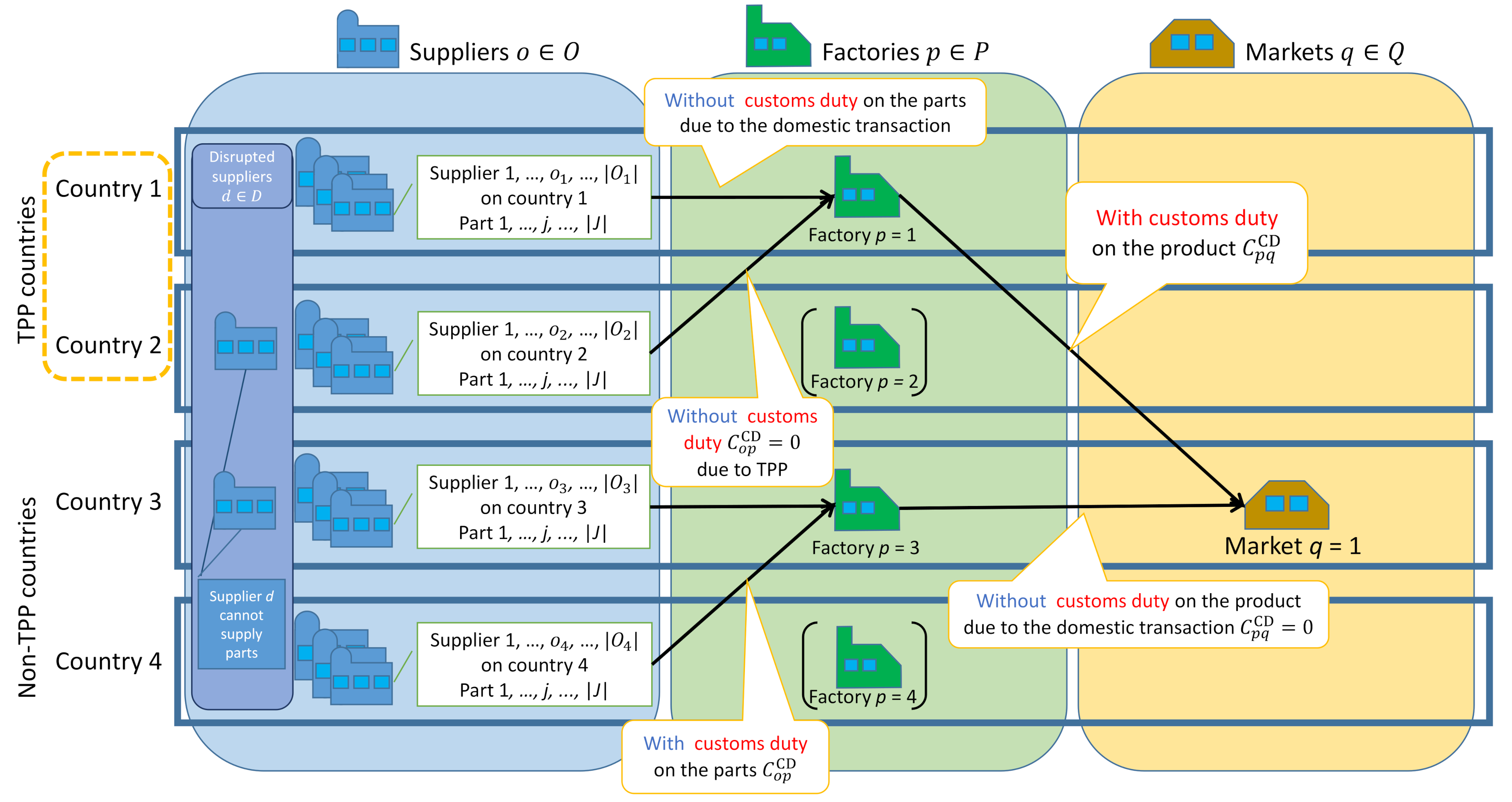
3.1. Model

The proposed model in this study is built and validated by integrating models from three previous studies. First, Nakamura et al.’s [20] model of a basic global supply chain with custom duty and BOM is used. Second, a global supply chain embedded with TPP, as modeled by Hayashi et al., is considered [21]. Finally, the disruption is modeled based on how it is incorporated by Nagao et al. [6]. Furthermore, the validation of the proposed model is verified through a numerical experiment. Figure 2 shows a global supply chain network with supply disruptions and the TPP. Here, part j is produced by supplier o and transported to factory p. Then, the finished product, consisting of Nj type parts, is assembled in factory p. Finally, finished products are transported to market q.
The global supply chain network with supply disruption and the TPP is modeled as follows: Given that supplier cities face the possibility of disruption, it would be impossible to supply parts to factory p. In this model, supplier d from a set of disrupted supplier cities D cannot supply any parts to factory p. Therefore, parts can only be transported from non-disrupted supplier o. In the disruption scenario where the world is affected concurrently, alternate/multi-sourcing is effective because the duration of the COVID-19 infection peak affecting disruption is different in different in countries [31,32].
Customs duties are imposed when parts or products are imported from outside the country. With respect to the TPP, customs duties, suppliers, factories, and markets are located in a set of countries. Group G defines a set of supplier cities in TPP countries. If a non-TPP country decides to trade with a TPP country, customs duty will be imposed by each country if both countries are not on the TPP list G. Of course, when trade is carried out between the countries that fall under the TPP, they are not required to pay the customs duty at each other’s borders.
This proposed model is applied at the strategic planning stage of a global supply chain, following Urata et al. [33], where a just-in-time environment is assumed in this study, which represents fewer inventory operations. Thus, inventory control, including lead time, is outside the scope of this study.
The notations used in this study are as follows:
Sets:
  • O: Set of suppliers, oO
  • O n : Set of suppliers on county n, O n O
  • G: Set of suppliers in countries forming the TPP, gG
  • D: Set of disrupted supplier cities in supplier set O, d D ,   D O
  • J: Set of parts, jJ
  • P: Set of factories, pP
  • Q: Set of markets, qQ
Decision variables:
  • v o p j : Number of parts j transported from supplier o to factory p
  • v p q : Number of products transported from factory p to market q
  • k p : Number of products manufactured in factory p
  • z p q : Binary value: 1 if the route between factory p and market q is opened, and 0 otherwise
  • u p : Binary value: 1 if factory p is opened, and 0 otherwise
Evaluation:
  • TC: Total cost [USD]
Cost parameters:
  • C o p L C : Logistics cost per unit part for transporting from supplier o to factory p
  • C p q L C : Logistics cost per unit product for transporting from factory p to market q
  • C o j P C : Procurement cost of procuring per unit part j by supplier o
  • C o p C D : Customs duty per unit on transportation from supplier o to factory p
  • C p q C D : Customs duty per unit on transportation from factory p to market q
  • C p M F : Manufacturing cost per product at factory p
  • C p q O R : Fixed cost for opening route between factory p and market q
  • C p O F : Fixed cost of opening factory p
Production parameters:
  • N j : Total number of parts j, consisting of one product
  • N q : Demand for products in market q
  • M: Very large number (Big M)
  • S p   : Production capacity at factory p
  • S o j   : Binary value: 1 if part j is supplied by supplier o, and 0 otherwise

3.2. Formulation

The global supply chain network is formulated as integer programming (IP) [34] based on Hayashi et al. [21] and Nagao et al. [6]. IP is well known as an appropriate way to adapt a global supply chain network to a transportation problem because it can be treated as linear programming, which enables us to solve large-scale problems [34]. The objective function of this study is to minimize the total cost of production TC, including transportation, procurement, customs duty, route opening, and factory opening costs, as shown in Equation (1).
Equation (2) stands for the condition that all of parts from the assigned suppliers meets the demand for all parts. Equation (3) means the constraint for all finished product at factory p is transported to markets. Equation (4) show the constraints that the number of finished products in market q transported to factories satisfies the demand. Equation (5) defines a constraint on a supplier as leading to supply disruptions when the supplier d belonging to a disrupted city D cannot supply parts to the factory. Equation (6) gives the production capacity of factories, while Equation (7) means the constraint for allowing transportation only through opened routes from factories to markets. Equations (8) and (9) set the binary restrictions for opening routes and factories and non-negativity for number of parts and products, respectively.
Objective function:
T C = o O p P j J ( C o p LC + C o j PC + C o j PC C o p CD ) v o p j + p P q Q C p q LC + C p MF + C p MF C p q CD   v p q + p P q Q C p q OR z p q + p P C p OF u p     m i n
Constraints:
o O S o j v o p j = N j k p           p P ,       j J
q Q v p q = k p           p P
p P v p q = N q             q Q
j J p P v d p j = 0           d D
q Q v p q F p u p           p P
v p q M z p q         p P ,       q Q
z p q , u p = 1 , 0         p P ,       q Q .  
v o p j ,   v p q 0       o O ,       p P ,       j J ,       q Q

4. Disruption Scenarios

To analyze the effect of supply disruptions in countries with and without the TPP in a global supply chain, this study considers an example of a global supply chain for a vacuum cleaner [35] with 23 types of parts, as in Hayashi et al. [21]. The product and supply chain data used for the numerical experiments are also based on Hayashi et al. [21] and were collected and assumed before the COVID-19 pandemic except disruption scenarios.

4.1. Global Supply Chain and Product Example

Figure 3 describes a global supply chain example and the setting. The details of global supply chain and product example are prepared as follows:
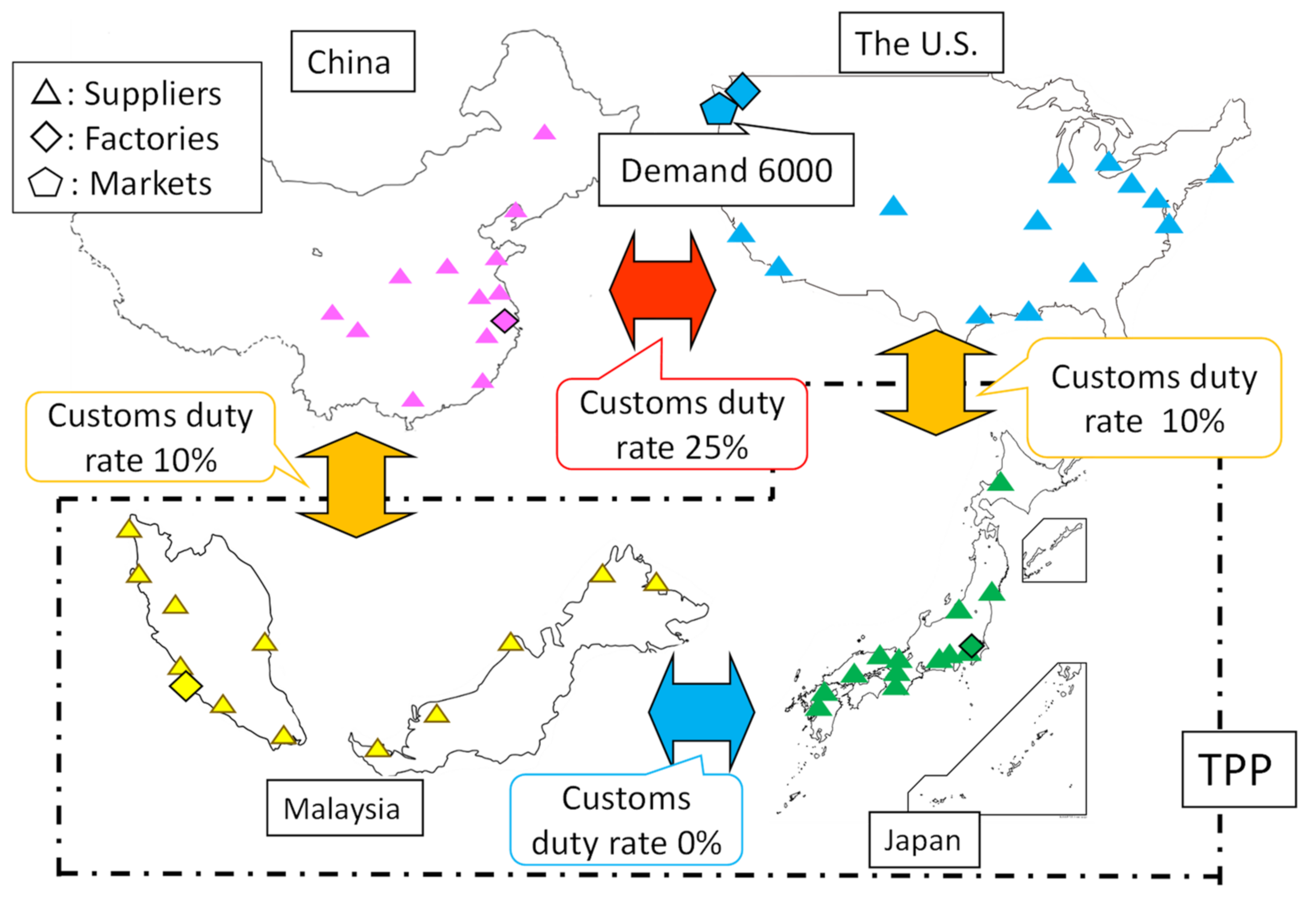
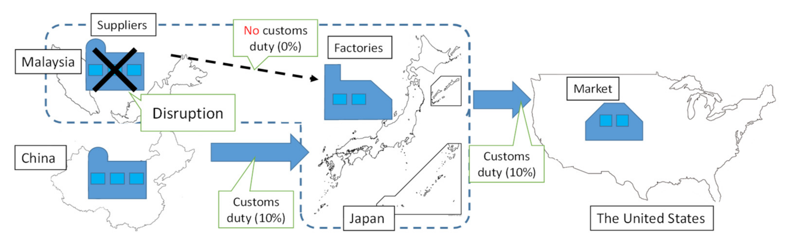
  • A total of 52 cities (13 cities in four countries, the U.S., China, Japan, and Malaysia) are selected as suppliers. Transportation costs of parts between cities are provided based on the distances as shown in Table A1 in Appendix A.
  • Four cities (Shanghai, Kuala Lumpur, Seattle, and Tokyo) are identified as candidate locations for factories. The production capacity of a factory is 3000 units. The market is set in Seattle in the U.S., and the demand is 6000 units of product. Transportation costs of product between factory cities and market cities are provided based on the distances as shown in Table A2 in Appendix A.
  • Japan and Malaysia are CPTPP member countries; in contrast, the U.S. and China are non-CPTPP member countries in the experiments. The customs duty between the U.S. and China is set at 25%. Between a CPTPP country and a non-CPTPP country, a duty of 10% is imposed. For instance, the customs duty between Malaysia and China, and between Japan and the U.S., is 10%. Meanwhile, customs duty is not imposed between CPTPP countries such as Malaysia and Japan.
Figure 4 illustrates the situation of the numerical experiments. A global supply chain under disruption with a customs duty and the TPP is considered. When the supplier in a TPP country, such as Malaysia, is disrupted, the factory may consider switching to suppliers from other countries such as China, Japan, and the U.S. Therefore, the customs duty cost increases because the customs duty rate increases from 0% to 10% or 25%.
Regarding product example (Table A3 in Appendix A), the average procurement price of the parts and manufacturing cost of the product in each country are shown in Table 2. The procurement cost of parts is calculated using the Asian international input/output table [36] and each part’s weight and price level (Table A4 in Appendix A), as in Hayashi et al. [21]. The manufacturing cost of the product is also similar to that in Hayashi et al. [21], and is calculated by Japanese cost and ratio of gross domestic product to other countries, which are the U.S., China, and Malaysia [37].

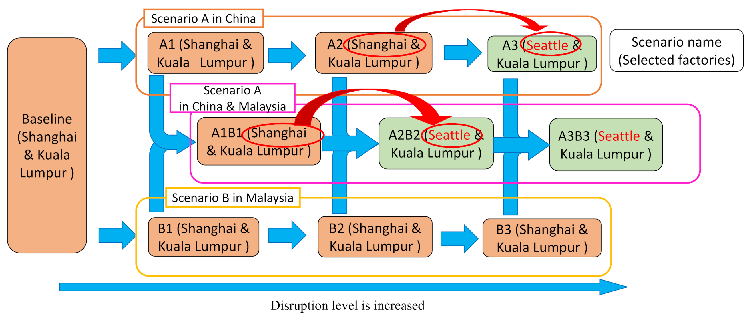
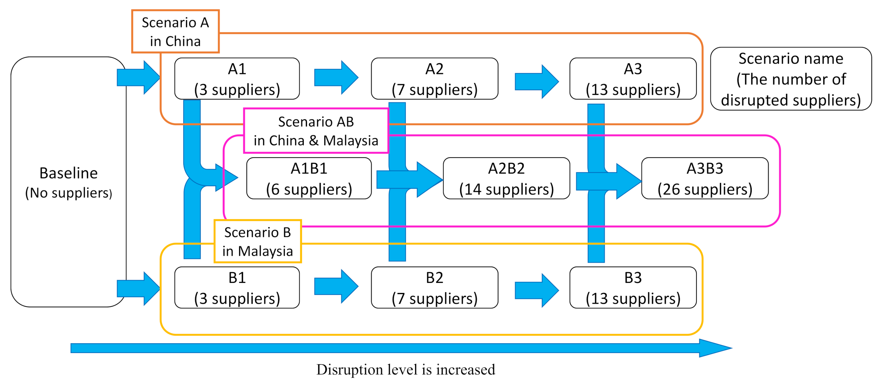
4.2. Example of a Disruption Scenario

To evaluate the impact of supplier disruptions, this study considers three disruption scenarios: one in China [30], a non-TPP country; the other in Malaysia, a TPP country; and the last one in both China and Malaysia. The sequence of the disruptions is shown in Figure 5. It is assumed that the government decides whether the city is disrupted. Here, we consider different TPP and non-TPP countries in the scenarios. For instance, if a disruption occurs in Japan, which is a TPP country, there are many suppliers located in Japan. Therefore, the customer must identify whether it is feasible for them to order some parts from a non-TPP country, although they will have to pay customs duty for that. Even when there is a disruption in TPP countries such as Malaysia and Japan, they can still import and export their products without extra customs duty costs because of the effects of the TPP.
The area disrupted by COVID-19 increases in scale and covers the entire country as follows: For example, in scenario A, supplier disruption happens in China, which is a non-TPP country. Scenario A1 refers to the disruption in three cities (Xian, Chengdu, and Chongqing). Next, in scenario A2, in addition to these three cities, four other cities—Nanjing, Hangzhou, Jinan, and Suzhou—are disrupted. Finally, all cities in China are disrupted in scenario A3. Scenario AB are set to analyze the combined impact of scenarios A and B simultaneously. The details of each scenario are prepared as follow:
  • Baseline: No disruption
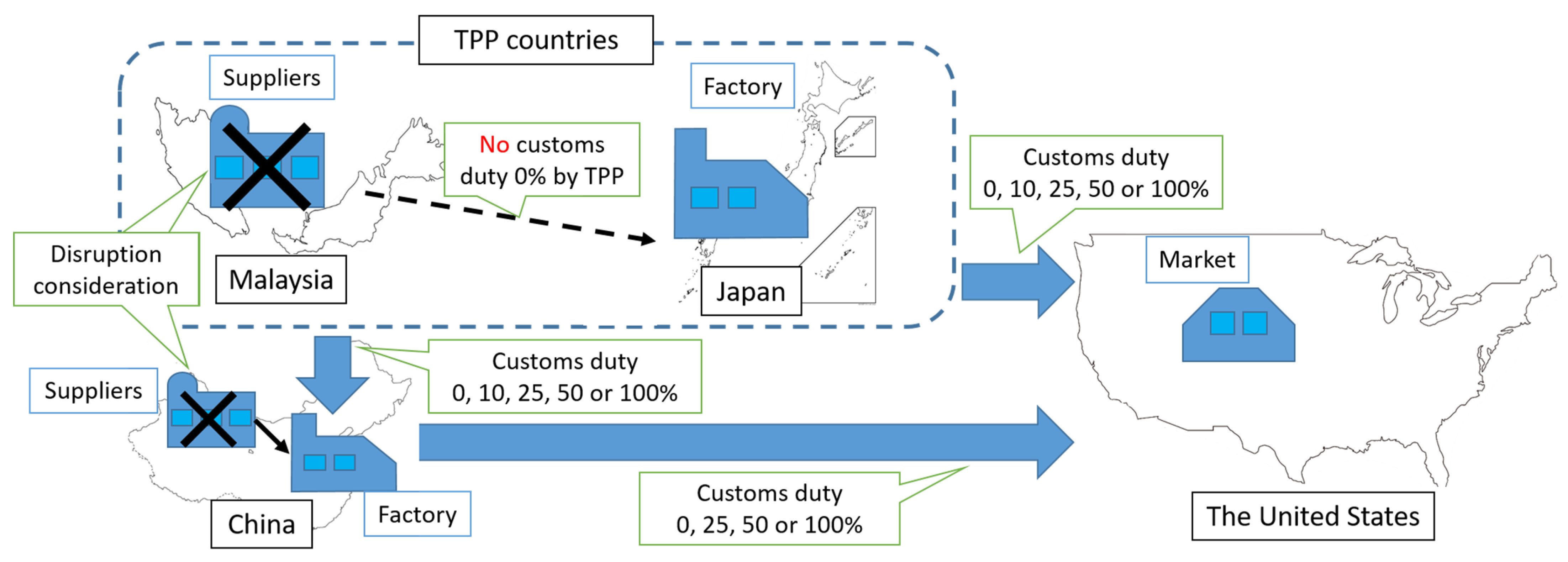
  • Scenario A: Supplier disruption in China, a non-TPP country.
    • A1: Disruption in three cities (Xi’an, Chengdu, and Chongqing)
    • A2: Disruption in seven cities (three cities in A1 + Nanjing, Hangzhou, Jinan, and Suzhou)
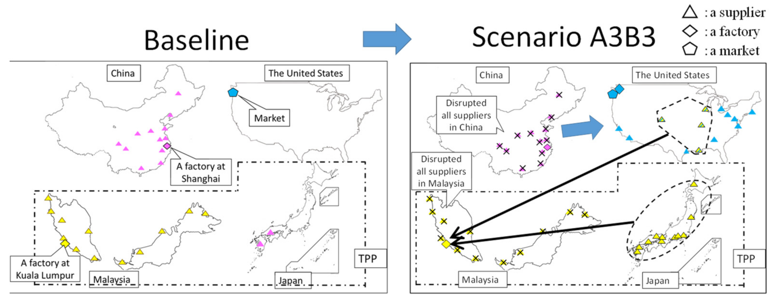
    • A3: Disruption of all Chinese suppliers
  • Scenario B: Supplier disruption in Malaysia, a TPP country.
    • B1: Disruption in three cities (Miri, Kota Kinabalu, and Sandakan)
    • B2: Disruption in seven cities (three cities in B1 + Kuantan, Johor Bahru, Kuching, and Sibu)
    • B3: Disruption of all Malaysian suppliers
  • Scenario AB: the combination of scenarios A and B.
    • A1B1: The combination of scenarios A1 and B1.
    • A2B2: The combination of scenarios A2 and B2.
    • A3B3: The combination of scenarios A3 and B3.
The numerical experiments were conducted using the optimization solver Numerical Optimizer [38] on an Intel® Core™ i5-4300U CPU @ 1.90 GHz PC with Windows 10 Pro.

5. Results: Impact on Combined Disruption Scenarios with and without TPP Countries

In this Section 5, numerical experiments are conducted by the proposed model with disruption scenario in Section 4. Section 5.1 describes the result of total cost. Section 5.2 considers the degree of disruptions and the countermeasure. Section 5.3 analyzes the impact of disruption on supplier selection without factory relocation.

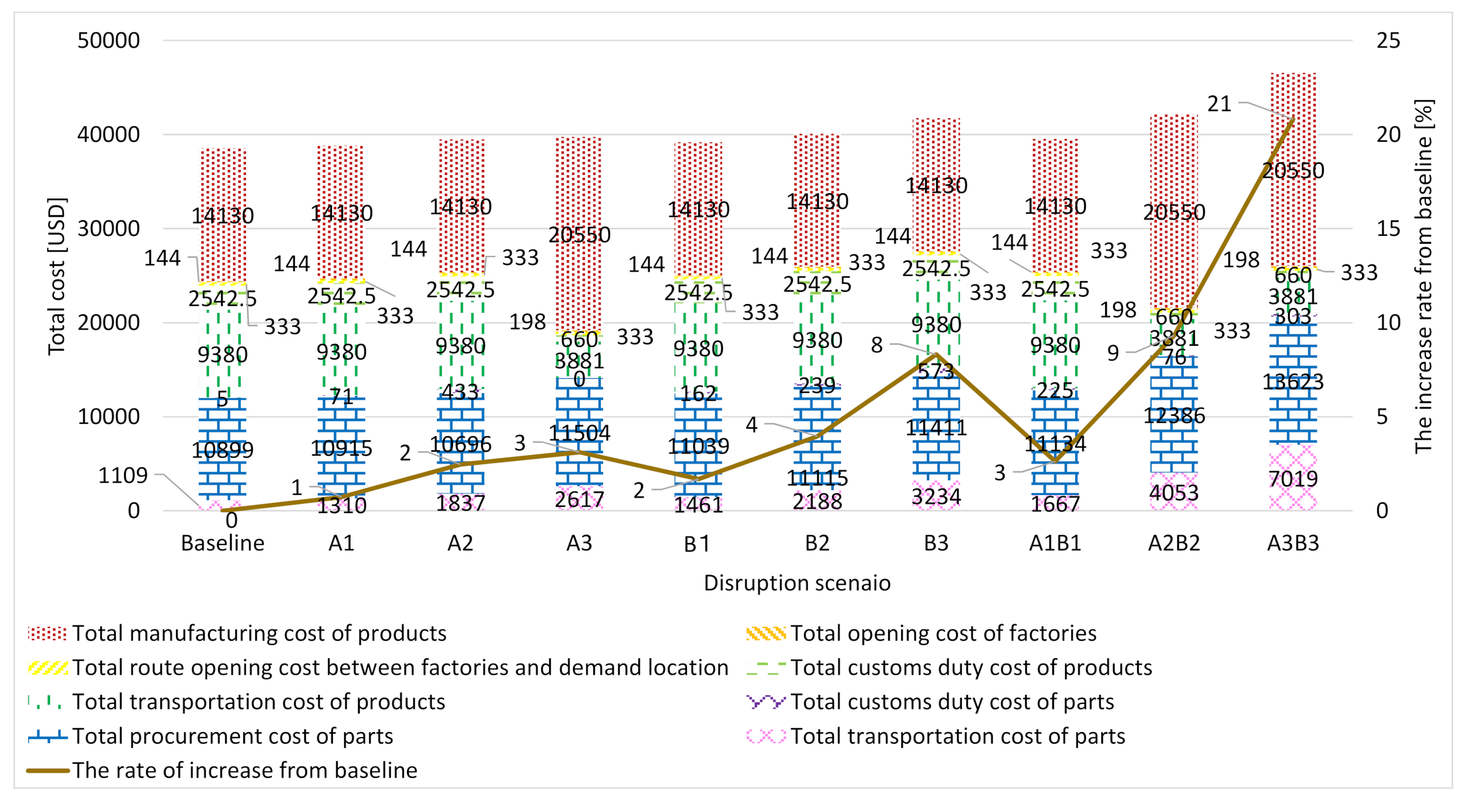
5.1. Results of Total Cost in Nine Scenarios

Firstly, total cost of each scenario is analyzed in order to evaluate economic impacts of disruption. Figure 6 shows the result of the total cost and the breakdown in each scenario. At the baseline, the total cost is USD 38,543. The trade relations and economic factors before the disruption caused by COVID-19 are that suppliers are selected mainly from China for the Shanghai factory, and from only Malaysia for the Kuala Lumpur factory. Parts #2 (wheel stopper) and #7 (switch) are supplied from Japan to the Shanghai factory. This is because their procurement costs are reasonable, even when the parts are supplied from Japan. Another reason is that their transportation costs from suppliers in China and Japan to the Shanghai factory are almost the same, as China is geographically expansive. The total cost mainly consists of the manufacturing cost for the product, the procurement cost for the parts, and the transportation cost for the product, at 36.7%, 28.3%, and 24.3%, respectively.
Regarding the breakdown of cost, the total customs duty of the parts in scenario A1 increases by 15 times from the baseline. However, in scenario B1, it increases by 34 times, because the transaction between Kuala Lumpur (in a TPP country) and the Chinese suppliers (a non-TPP country) increases by five types of parts. Chinese suppliers were selected over Japanese suppliers for this factory while Japanese suppliers were not chosen because of their high procurement costs. Thus, for low-level disruption cases, such as A1 and B1, cost suppression, as with the low procurement cost of China, is more effective than savings in customs duty through the TPP.
For scenario A1B1 (six cities’ disruption), the total cost increases by 2.6% compared to the baseline; this is almost equal to the 2.5% increase for scenario A2 (seven cities’ disruption), but much lower than the 4.0% increase for scenario B2 (seven cities’ disruption). For scenario A2B3 (14 cities’ disruption), the total cost increases by 9.3% from the baseline; this is higher than the 3.1% for scenario A3 (13 cities’ disruption) and 8.3% for scenario B3 (13 cities’ disruption). Thus, when small disruptions occur simultaneously in multiple countries, the impact on costs is as small as, or even smaller than, that for medium disruptions within a country. However, when medium disruptions occur in more than one country, the cost impact is greater than when all cities in a country are disrupted.
Figure 7 shows the results of redesigning the global supply chain network from the baseline to scenario A3B3. Japanese suppliers are selected for Malaysian factories because all Malaysian suppliers are disrupted in scenario A3B3. Therefore, 58% of the total customs duty costs of parts are saved by the TPP.

5.2. The Degree of Disruptions and the Countermeasure

Figure 8 shows the results for the selected factories in each scenario. As shown in Figure 8, the need to relocate a factory depends on the estimated possibility of disruption. Specifically, for low-level disruptions, the same factory as in the baseline scenario is selected, and disruptions may be dealt with by switching suppliers. However, as the disruption level increases, the factory may relocate from Shanghai to Seattle.
This Figure 8 also provides practical suggestions for the relocation of factories when the disruption level is expected to increase. Assuming that Chinese suppliers can recover quickly, the choice of factory location in Shanghai and Kuala Lumpur will depend on the overall disruption scenario. This is because the disruption of Chinese suppliers will prompt the factory to move to Seattle; however, once the Chinese supplier is restored, the optimal factory location will again be Shanghai. Therefore, disruption has a higher cost impact in Malaysia than in China. This may be because Malaysia has the lowest procurement cost for all parts at that time. Thus, assuming that Chinese suppliers recover quickly, the choice of factories in Shanghai and Kuala Lumpur will be effective when considering the overall disruption scenarios as shown in Figure 8.

5.3. Impact of Disruption on Supplier Selection without Factory Relocation

In contrast to Section 5.2, which addresses the cases where factories can be relocated, in this section, the cases in which factories cannot be relocated are analyzed. Figure 9 shows the changes in costs in different scenarios with and without factory relocation, while Table 3 compares the factory and supplier choices. As shown in Figure 9, the total cost in scenarios A3 and A2B2 increases by 0.7% when the factory is not relocated, compared to when it is. In scenario A3, the main reason for this is that the total transportation cost of products, total customs duty of products, and total customs duty of parts increase by USD 5499, USD 1883, and USD 556, respectively. However, the overall increase in the total cost is only 0.7% because the cost breakdown across different costs changes: Seattle is chosen as the best location for an opening factory under total cost minimization; however, suppliers from Japan and Malaysia are consequently selected to reduce the total procurement and transportation costs of parts.
A similar phenomenon occurs in scenario A2B2. However, in scenario A3B3, the total cost increases significantly, by 6.3%. This could be mainly due to the increase in total procurement cost of parts by USD 1062, which, rather, decreases in scenarios A3 and A2B2, and the increment in the total customs duty of parts by USD 1157, which only increases by approximately USD 500 in both scenarios A3 and A2B2. From Table 3, the factory remains unchanged in scenario A3B3, and almost all factory suppliers in Shanghai and Kuala Lumpur factories become Japanese because the Chinese and Malaysian suppliers discontinue supplying the parts during the disruption. It is noted that the total procurement cost of parts increases because of the increase in Japanese suppliers. The customs duty of parts depends on their procurement cost; therefore, with a higher customs duty, the total customs duty of parts is increased.
These results show that the increment rate in the total cost for maintaining the factory in operation without relocation depends greatly on the scenario. When the factory is not relocated, the increment in total cost can be reduced by choosing cheaper alternative suppliers. However, the cost increment is significant in the case of very large disruptions.

6. Analysis of Disruption Impact: Non-TPP vs. TPP Countries

In Section 5, the impact of disruption was analyzed. This Section 6 discusses the TPP effects by contrasting the result of TPP versus non-TPP countries disruption. Firstly, in Section 6.1, the minimum scale disruption scenarios A1 and B1 in this study are compared and analyzed. Next, Section 6.2 explains the result of non-TPP country disruption in detail. Finally, we conclude the supplier selection under the supplier disruption.

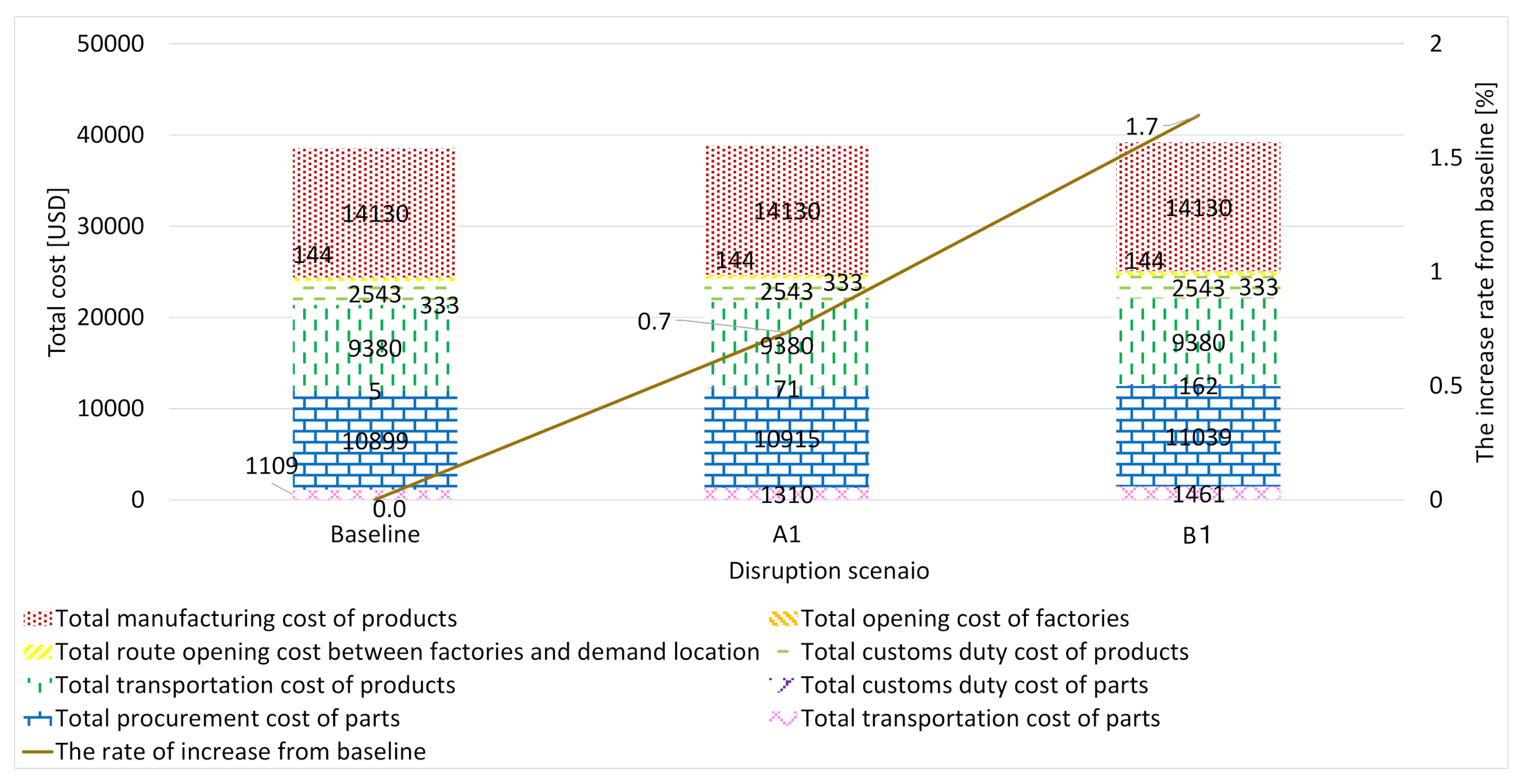
6.1. Comparison of Results of the Disruption Scenarios A1 on a Non-TPP Country and B1 on a TPP One

To determine the disruption impact on TPP and non-TPP countries, this section analyzes the difference in disruption impact between China and Malaysia through a numerical experiment conducted on the total cost minimization presented in Section 5.
Table 4 shows the selection results for suppliers and factories in disruption scenarios A1 on a non-TPP country and B1 on a TPP one. In all cases, factories are not relocated from Shanghai and Kuala Lumpur at baseline. However, the selection results for suppliers differ for each case. In scenario A1, with disruptions of three Chinese suppliers of the Shanghai factory, three Malaysian and four Japanese suppliers are selected for the three disrupted Chinese suppliers. One reason for this is that out of the four countries, the procurement cost for suppliers is the lowest in Malaysia. However, four Japanese suppliers are also selected because the transportation cost to Shanghai is lower in Japan than that from Kuala Lumpur in Malaysia owing to a shorter travel distance, even though their procurement cost is higher than that of Malaysian suppliers.
Regarding scenario B1, four Chinese suppliers are selected instead of the three disrupted Malaysian suppliers. However, Japanese and U.S. suppliers are not selected because of their higher procurement costs.
Figure 10 shows the results of the total cost at the baseline, and at scenarios A1 and B1. The difference in the total cost between the baseline and the scenarios is only approximately 1%. Thus, when the disruption is as small as three cities, whether in China or Malaysia, switching from the disrupted supplier to other suppliers is recommended rather than changing the factory.

6.2. The Impact of Non-TPP Country Disruption

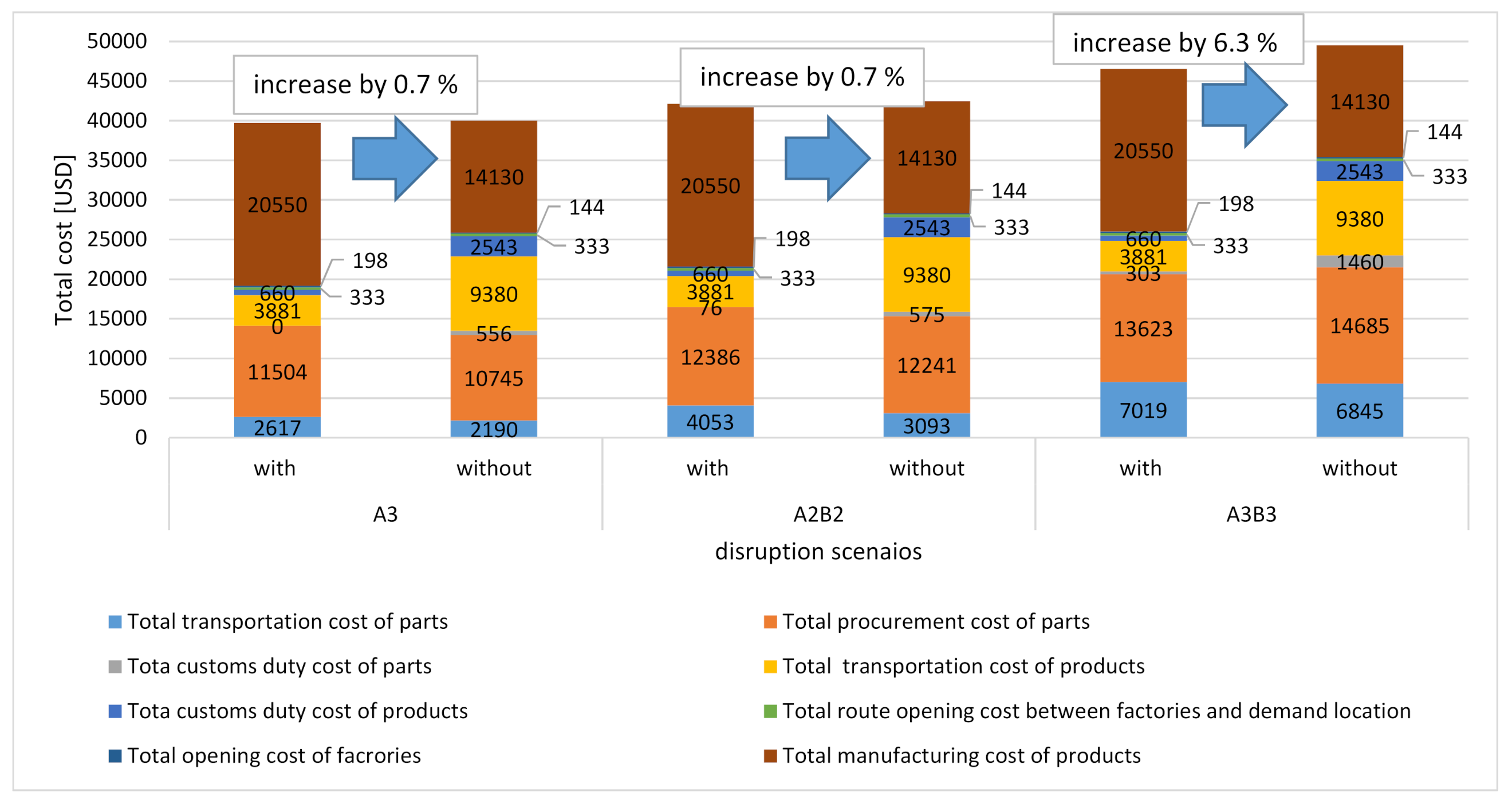
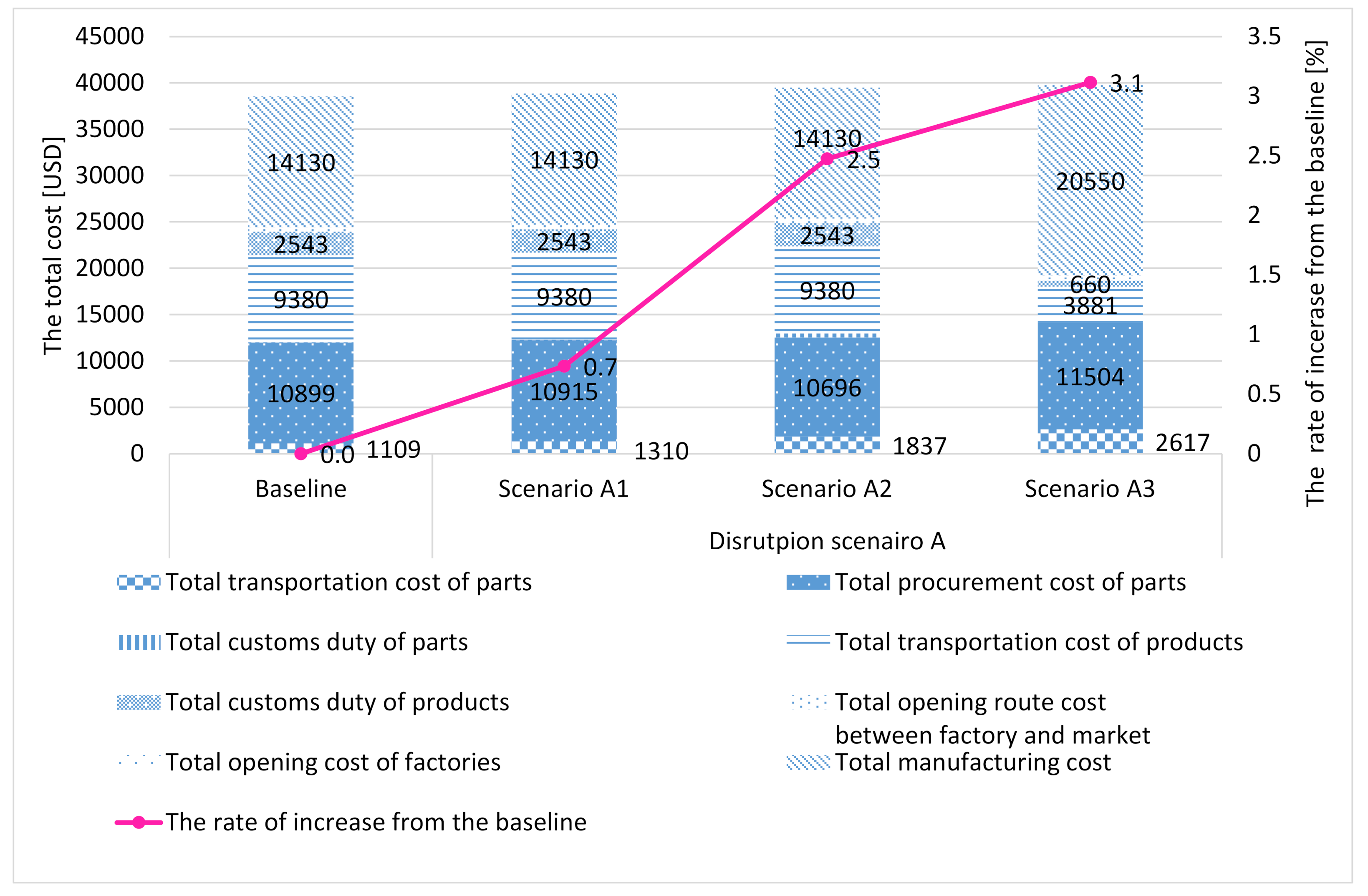
6.2.1. The Impact on Total Cost and the Breakdown

To investigate the impact of non-TPP country disruption, this section shows the results of Chinese supplier disruptions. The results of the selection of suppliers and factories in scenario A are shown in Table 5. Figure 11 shows the total costs and its rates of increase in scenario A. The total cost in scenario A3 increases by 3.1% compared to the baseline. This is a result of the redesign of the global supply chain by relocating factories and suppliers because of supplier disruptions in China. Specifically, by moving the factory from Shanghai to Seattle in the U.S., where the market is located, parts are supplied from U.S. suppliers, while the total customs duty of the parts, total customs duty of the products, and total product transportation cost decrease by 100.00%, 58.63%, and 74.04%, respectively.
As the scale of disruptions increases in scenarios A1, A2, and A3, the total part transportation cost increases by 18.1%, 65.6%, and 135.9%, respectively. This is because the number of suppliers outside China increases due to disruptions. For instance, as shown in Table 5, three Chinese supplier cities are not selected because of the disruption, and three and four new suppliers from Malaysia and Japan, respectively, are selected in scenario A1. Similarly, in scenario A2, seven Chinese suppliers are not selected because of disruptions, and six suppliers from Malaysia and five suppliers from Japan are selected instead. Thus, Japanese suppliers with higher procurement costs are selected because the transportation cost from the Japanese supplier to the Shanghai factory is lower than that from Malaysian suppliers. Therefore, the Japanese supplier is expected to be selected for parts with lower procurement and transportation costs.
Moreover, the total part procurement cost increases by 0.14% in scenario A1, while it decreases by 1.9% in scenario A2 as shown in Figure 11. This is because disruptions lead to the selection of suppliers in Malaysia, where procurement costs for all parts are lower than in Japan and the U.S., instead of suppliers in China. In scenario A3, the total part procurement cost increases significantly by 5.60% compared to the other scenarios because the factory is moved to Seattle in the U.S., where the market is located; thus, all suppliers are selected from the U.S.
In addition, the total customs duty cost increases substantially, by 15 and 93 times in scenarios A1 and A2, respectively. This increase is due to the change in the choice of suppliers from the country of the factory to a foreign supplier upon disruption. In contrast, in scenario A3, the total customs duty cost of the product reduces by 100% because the factory is moved to Seattle, U.S., where the market is located; moreover, the total customs duty cost of the product is completely eliminated. It means that supplier disruptions significantly impact customs duty costs. However, the ratio of total customs duty cost of parts to total cost at the baseline is only 0.01%; furthermore, the impact of supplier disruptions on the total customs duty cost of the parts is greatest in scenario A2 among disruptions in China, at 1.12% of the total cost.
Hence, the total transportation cost of the products, total customs duty costs of products, factory opening costs, and total manufacturing costs remain unchanged in scenarios A1 and A2. However, in scenario A3, the costs change as the factory moves from Shanghai to Seattle. Specifically, the total product transportation costs and total customs duty of the products decrease by 58.6% and 74%, respectively, while the factory opening costs and total manufacturing costs increase to 35.80% and 54.50%, respectively. The factory moves from Shanghai to the U.S. where the market existed. However, the U.S. has a large landmass; this increases the domestic transportation costs, and thus, the total product transportation costs. Here, the domestic transportation cost is higher than the total transportation cost when the parts are imported. Therefore, the effects of supplier disruptions significantly impact factory relocation and costs, such as transportation costs of the product and parts, and customs duty costs of the product and parts.

6.2.2. The Impact on Supplier Selection under Supply Disruption

In scenarios A1 and A2, the factories are the same as the baseline (i.e., Shanghai and Kuala Lumpur). In scenario A1, the Chinese suppliers are removed as they are disrupted; instead, three new suppliers from Malaysia and two from Japan are selected. In scenario A2, more disrupted Chinese suppliers are removed; however, besides the suppliers selected in scenario A1, new suppliers are selected in three cities from Malaysia and one from Japan. There is no change in the choice of suppliers to the factory in Kuala Lumpur in scenarios A1 and A2. In scenario A3, the factory is relocated from Shanghai to Seattle. This means that all suppliers are in the same country as the selected factory. These results indicate that there is no effect on the supplier’s selection if the disruption occurs in a country different from the factory.
There are two types of factors for supplier selection. The first type is the direct effect of supplier disruptions. For example, as shown in Table 5, suppliers are switched for the factory in Shanghai in scenarios A1 and A2. Then, the total cost of the parts is expected to increase as shown in Figure 11 because the best suppliers are not chosen due to the disruption. The second type of factor is the indirect influence of factory relocation. For example, as shown in Table 5, suppliers for the factory at Seattle are the case in scenario A3. Then, the total manufacturing cost of products is expected to increase, as shown in Figure 11. This is because relocating a factory means moving the factory from the best factory location at the baseline to another location.

7. The Effect of the Customs Duty Rate Changes

This section deals with the impact of custom duty rate. Section 7.1 summaries the result of total custom duty cost in each scenario. Next, Section 7.2 describes the influences of changing custom duty rate on factory and supplier selection under disruption in Malaysia. Finally, Section 7.3 conducts sensitivity analysis for custom duty under the Malaysian disruption scenario in order to analyze the relationship between custom duty rates and supplier selection.

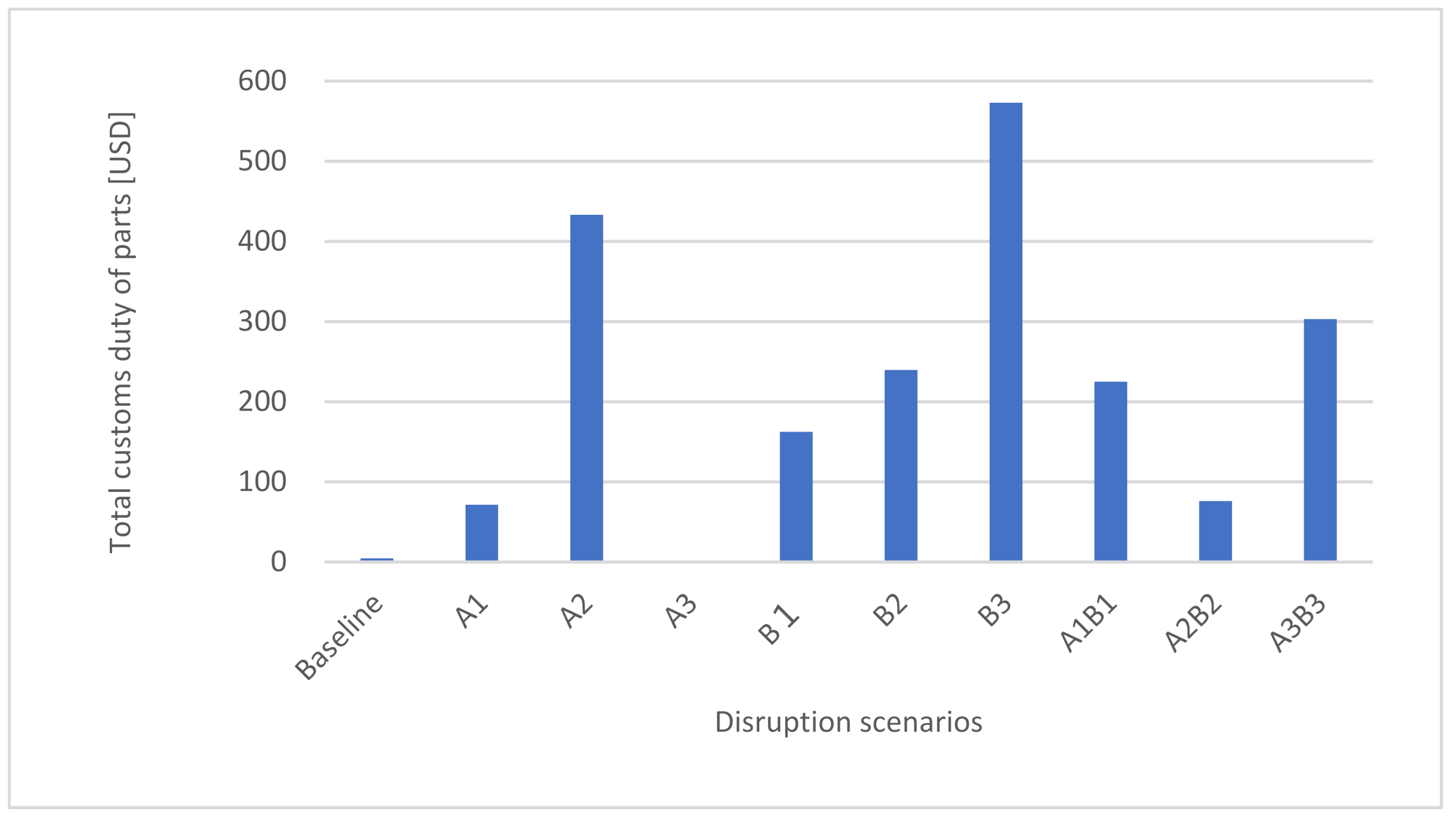
7.1. Total Customs Duty Cost by Each Scenario

This section discusses the customs duty cost and the effect of the TPP under disruption scenario B.
Figure 12 shows the results of the total customs duty cost of the parts in all scenarios. The total customs duty cost of parts in scenario A3B3 is lower than that in scenarios A2 and B3 by 30% and 47%, respectively. This is because the customs duty cost is zero between TPP participants, which are Japan and Malaysia in this set. In scenario A3B3, one of the factories is selected from Kuala Lumpur, and most of the suppliers are in Japan. Therefore, even though the disruption scale of scenario A3B3 is the largest among all scenarios, the total customs duty cost of parts is not the highest because of the effect of the TPP. Thus, this is an example which implies that the TPP has a good influence on economizing expenses in a situation with disruption.

7.2. Impact of Customs Duty Rate Changes on Factory and Supplier Selection under Malaysian Disruption Scenarios B

In this section, the selection of the supplier and the factory are analyzed under different customs duties through Malaysian disruption scenarios.
Table 6 shows the changes in factories and suppliers due to the Malaysian disruption scenarios and changes in customs duty rates. In the baseline (i.e., scenarios B1 and B2), the factories in Shanghai and Kuala Lumpur (Kuala Lumpur and Seattle) are selected when the customs duty rates are 10% and 25% (50% and 100%), respectively. The factory is moved from Shanghai to Seattle to reduce the product customs duty cost because the aim is to manufacture the product in the same country as the market. Regarding the choice of factories in scenario B3, Shanghai and Kuala Lumpur (Shanghai and Seattle) are selected when the customs duty rates are 10% and 25% (50% and 100%), respectively.
When the customs duty rate is approximately 10% or 25%, even if all Malaysian suppliers are disrupted, it will be less expensive to procure parts from Chinese suppliers and manufacture the product in the Kuala Lumpur factory. However, when the customs duty rate is 50% or more, the factory moves from Kuala Lumpur to Seattle to avoid the impact of customs duty on the import of parts and products.

7.3. Sensitivity Analysis by Customs Duty Rate in Scenario B

Finally, to analyze the effect of TPP, sensitivity analysis by customs duty rate is performed to the extent that the factory is not moved.
Table 7 shows the resulting total and breakdown costs in the sensitivity analysis by customs duty rate from 41% to 100% in scenario B1. Notably, an increase in the customs duty rate from 41% to 100% significantly increases the total cost by 9.69%.
Table 7 also shows that the increment in customs duty rate does not affect the total transportation cost of products, the cost of establishing a route between factories and markets, and the total manufacturing cost. This is because factory relocation does not occur within the scope of this sensitivity analysis.
The total transportation and procurement costs of parts increase by 6.78% and 6.13%, respectively, with an increment in the customs duty rate from 41% to 100%. The relocation of suppliers from China to Japan perhaps increases the total transportation cost of parts due to the greater distance between the factory in Kuala Lumpur and suppliers. Furthermore, the total parts procurement cost increases because of the higher procurement cost of parts in Japan than in China.
The total customs duty cost of the product increases by 143.90%, while the total customs duty of parts decreases by 100.00% as the customs duty rate increases from 41% to 100%. The significant reduction in the total customs duty of parts is because Japan is selected as the supplier for the factory in Kuala Lumpur, where both Japan and Kuala Lumpur are within the TPP region. Therefore, in some cases, belonging to the TPP is effective in controlling the customs duty cost of parts.
Table 8 shows the customs duty rates and the choice of foreign suppliers for the Kuala Lumpur factory, where red and blue cells are for Chinese and Japanese suppliers, respectively. Parts #9, #10, #11, #17, and #21 were selected from suppliers outside Malaysia because of the disruption of suppliers in Malaysia in scenario B1. It is noticed that the number of Chinese (Japanese) suppliers selected decreases (increases) as the customs duty rate increases. Therefore, imports between countries belonging to the TPP are not affected by an increase in the customs duty rate imposed on imports of parts and products. Furthermore, in some cases, Japanese suppliers are more likely to be chosen as suppliers to a factory in Kuala Lumpur, especially in the event of a large increase in customs rates.

8. Discussion

This section summarizes the findings of the numerical experiments in Section 5, Section 6 and Section 7. Based on the results, the discussions here are outlined in terms of the nature of disruption, such as the size, duration, impact, and aftermath, as follows:
  • Size: The disruption scale affects the total cost increment and the factory relocation from one of the selected factories at baseline, which is in China, to the market country, which is in the US.
  • Duration: The duration is not directly considered in the numerical experiment. However, by assuming the sequences of different locations and sizes of disruption, as shown in Figure 5 and Figure 8, the disruption duration can be considered through the numerical experiment. Thus, some practical recommendations emerge from the results. First, if the duration of Chinese supplier disruption is brief, such as a few months, the factory in China should not be relocated because of the relocation cost. Second, if the duration of Chinese supplier disruption is long, such as a few years, the factory in China should be relocated to the market location, Seattle.
  • Impact: The disruption impact differs by country. The large disruption including Chinese suppliers in scenarios A3, A2B2, and A3B3 causes factory relocation. Moreover, the relocation increases the manufacturing cost for the product because the price ratio and labor cost differ across countries. However, for Malaysian supplier disruptions, such as scenarios B1 to B3, the effect of disruption on factory relocation is not observed as suppliers are switched from the Malaysian suppliers to those from other countries.
  • Aftermath: Once a factory is relocated to avoid the disruption, the factory must be maintained even when the disruption ends. Therefore, decision makers should carefully consider whether facilities such as factories are should indeed be relocated. The duration of the disruption is an important factor in determining this as production can be stopped in brief disruptions. In contrast, the way of maintaining production by switching to alternative suppliers and relocating a factory should be undertaken in lengthier disruptions, such as that caused by COVID-19.
In addition, some practical recommendations emerge from the results. The Malaysian factory is maintained under all nine scenarios, even when all Malaysian suppliers are disrupted in the experiments. The results show that automation in a Malaysian factory is effective in suppressing the increase in total costs under COVID-19 induced disruptions. The disruption duration is not considered directly in the numerical experiments. However, if the duration of Chinese supplier disruption is brief, such as several months, the factory in China should not be relocated considering the relocation cost. Second, if the duration of Chinese supplier disruption is long, such as some years, the factory in China should be relocated to the market location, which is Seattle in the experiment.
Against a large disruption, reconfiguring a global supply chain is appropriate. This result supports the orientation of the entire supply chain management for economic effectiveness [23]. Switching to alternative suppliers is effective for maintaining production. Furthermore, more corporations, including SMEs, should take sustainability actions. This includes countermeasures against disruptions, regardless of their longevity, such as a business continuity plan [24]. Finally, a new way of developing resilience using new technology, such as blockchain [25], should be considered in future studies.

9. Conclusions and Future Research

This study examines the impact of supplier disruptions caused by COVID-19 on redesigning global supply chain networks across TPP countries using nine scenarios with different scales of disruption. The main findings are as follows.
  • The results of the nine disruption scenarios show that once the Chinese supplier is restored, the factory placement returns to Shanghai after the Chinese supplier disruption brings the factory to Seattle. Then, assuming the recovery speed of disrupted suppliers, strategic factory selection after the recovery of disruptions is proposed.
  • The behaviors of total and breakdown costs under different scales of disruptions are analyzed through the disruption scenarios in China. Regarding supplier selection, there are two patterns: directly changed by supplier disruption, and indirectly changed due to factory relocation. Depending on the scale of disruption and the locations of occurrence, the impact on total cost changes regardless of the number of disrupted suppliers.
  • Some potential scenarios are found where companies may or may not change their supply chain design due to fluctuations in duties and tariffs. Regarding the TPP effect, there is a case in which the TPP has a positive impact on maintaining costs despite disruption. Moreover, when the supplier disruption and the increment in the customs duty rate occurs simultaneously, there is a case in which suppliers in TPP countries are chosen to avoid an increase in customs duty costs.
  • Alternative suppliers in the other country should be selected instead of disrupted ones. Then, the factory should be maintained at the existing location. However, when many suppliers are switched from far alternative suppliers to the existing country because of the disruption, the factory should be relocated to the country in which the suppliers are selected. Moreover, the results indicate that the TPP has a positive impact on maintaining costs despite disruption; it is the non-TPP countries which affect costs as customs duty costs increase. Therefore, non-TPP countries are gradually selected less under the customs duty-rate increment and disruption. Emerging one managerial insight is that in the maintained factory, regardless of the disruption, a capital investment such as automation should be carried out. Then, the operation can be continued under the disruption by switching to alternative suppliers while suppressing the total cost increases.
Further studies should consider factory disruptions. This study analyzes supplier disruptions in a global supply chain. Considering the impact of factory disruption is necessary to design a robust global supply chain network. The other studies should also consider devising resilient system designs to quickly restore the global supply chain [39], and consider the lead time at the operational stage under the disruption. Lastly, as carbon taxes have been and are increasingly being implemented [33,40,41], future studies should consider this as well.

Author Contributions

T.N. and T.Y. conceptualized the goals and aims of this study, and provided resources. T.N., H.I., T.Y. and K.N. designed the methodology. T.Y. acquired funds. T.N. generated the metadata, and formulated and operated the numerical experiments. T.N. programmed and validated the formulation, and visualized the results with H.I. T.N. wrote the original draft assisted by H.I., L.Z. and T.Y. T.Y. managed this project and supervised the overall content, and H.I. reviewed the manuscript. T.N., H.I. and T.Y. revised the manuscript. All authors have read and agreed to the published version of the manuscript.

Funding

This study was partially supported by the Japan Society for the Promotion of Science (JSPS), KAKENHI, Grant-in-Aid for Scientific Research (A), JP18H03824, from 2018 to 2021.

Data Availability Statement

Not applicable.

Conflicts of Interest

The authors declare no conflict of interest.

Appendix A

Table A1. Transportation costs of parts between cities [USD].
ShanghaiKuala LumpurSeattleTokyo
Atlanta0.1229760000.1586400000.0350798000.110339000
Alor Star0.0355737200.0036261800.1272590000.051890640
Guangzhou0.0121324000.0255100000.1038880000.029056110
Fukuoka0.0087885600.0451467500.0844660000.008819450
San Jose0.0994630000.1365600000.0111837000.083314000
Penang0.0362788200.0027153300.1279600000.052476710
Chongqing0.0144363000.0298603500.1013530000.031651550
Hiroshima0.0108512000.0471518500.0826330000.006751860
Detroit0.1145955000.1493600000.0621138000.101157000
Kuantan0.0514900800.0019727600.1278750000.051490080
Nanjing0.0026996300.0368334100.0927300000.019689570
Yokohama0.0175030300.0530833100.0770940000.000277890
Chicago0.1135695000.1492160000.0281623000.113350000
Malacca0.0381064900.0012166300.1299290000.053625820
Harbin0.0168020600.0532811600.0766620000.015767770
Osaka0.0136444200.0495361700.0801110000.000396890
Cleveland0.1158440000.1503900000.0326887000.104493000
Kuala Lumpur0.0375338000.0000100000.1293590000.053276340
Xian0.0122205700.0355384500.0954340000.027962100
Nagoya0.0150133800.0508863300.0791330000.002588690
Boston0.1173285000.1490300000.0400522000.107891000
Johor Bahru0.0380236200.0029612600.1296940000.053162080
Chengdu0.0166259600.0306410500.1017000000.033508700
Sapporo0.0219203100.0599283500.0702690000.008330410
Pittsburgh0.1174395000.1516500000.0342962000.106259000
Kuching0.0360753000.0097939700.1254940000.048616730
Changchun0.0144131300.0509152800.0787040000.052302800
Kumamoto0.0088867800.0447733900.0849510000.008864890
Los Angeles0.1043065000.1413600000.0154517000.088101000
Sibu0.0337489600.0113272200.1238760000.046954700
Dalian0.0085543200.0446512400.0848550000.016375080
Kobe0.0133697000.0493116500.0806310000.004238580
Houston0.1219545000.1593100000.0306805000.107318000
Miri0.0309489100.0137362000.1205650000.043747360
Hangzhou0.0016506200.0359249600.0934250000.019173776
Shizuoka0.0162869700.0518465200.0783570000.001429900
New Orleans0.1243910000.1612800000.0339108000.110491000
Kota Kinabalu0.0286630100.0163181000.1177820000.040926890
Jinan0.0072486800.0405301200.0893830000.020265060
Kyoto0.0139607000.0499443700.0798570000.003641270
Washington0.1198285000.1533700000.0372490000.109014000
Sandakan0.0284823300.0184133200.1165460000.039917480
Qingdao0.0054781600.0413860200.0882100000.017392910
Sendai0.0193429600.0557604500.0741390000.003055610
Saint Louis0.1158195000.1521300000.0276538000.104495000
Ipoh0.0364901600.0017587800.1238180000.052512710
Suzhou0.0008487600.0370885700.0923520000.018364290
Niigata0.0176965800.5422528000.0756880000.002546620
Denver0.1078455000.1452400000.0163022000.093269000
Penang0.0362788200.0027153300.1279600000.052476710
Fuzhou0.0061204200.0317127900.0976950000.022165510
Wakayama0.0132423900.4898081000.0810140000.004432180
Note: Red, yellow, blue, and green marked cells mean Chinese, Malaysian, Japanese, and the U.S’s suppliers and factories, respectively.
Table A2. Transportation costs of product between factory and market cities [USD].
ShanghaiKuala LumpurSeattleTokyo
Shanghai0.0001000.3753381.8332080.176019
Kuala Lumpur0.3753380.0001001.2935900.532763
Seattle1.8332081.2935900.0001001.532334
Tokyo0.1760190.5327631.5323340.000100
Note: Red, yellow, blue, and green marked cells mean Chinese, Malaysian, Japanese, and the U.S’s factories and markets respectively.
Table A3. BOM of the parts and procurement costs.
Part No.Part NameRequired Number for a ProductProcurement Costs [USD]
The U.S.MalaysiaChinaJapan
1Wheel of nozzle20.01530.01260.01380.0196
2Wheel stopper20.00370.00300.00330.0047
3Upper nozzle10.05450.04480.04920.0698
4Lower nozzle10.04470.03670.04030.0572
5Nozzle10.03740.03070.03370.0478
6Right handle10.05300.04350.04780.0678
7Switch10.00410.00340.00370.0058
8Left handle10.05600.04600.05050.0716
9Left body10.20280.16670.18290.2595
10Right body10.19480.16010.17570.2493
11Dust case cover10.06290.05170.05670.0964
12Mesh filter10.32090.26370.28940.5990
13Connection pipe10.07810.06420.07050.1012
14Dust case10.30220.24830.27250.4632
15Exhaust tube10.02860.02350.02580.0401
16Upper filter10.30850.25350.27820.5759
17Lower filter10.03180.02610.02860.0406
18Protection cap10.03410.02800.03070.0437
20Rubber of outer flame of fan10.04220.03470.03810.0556
21Outer flame of fan10.09130.07500.08230.1182
22Lower fan10.01630.01340.01470.0209
23Fan10.10290.08450.09280.1332
Table A4. Comparison of price levels between nations, with Japan set as 1 (Ministry of Internal Affairs and Communications, 2011).
Price Level IndexEquipment Residential Devices Maintenance
Japan1
China0.57
The United States0.64
Malaysia0.52

References

  1. Kubo, M. Global supply chain optimization models. J. Jpn. Ind. Manag. Assoc. 2006, 16, 56–61. (In Japanese) [Google Scholar]
  2. JETRO. Jetro Trade Handbook 2017; Japan External Trade Organization: Tokyo, Japan, 2017. (In Japanese) [Google Scholar]
  3. JETRO. 40% of Japanese Companies in the U.S., Change Their Suppliers, from China to Japan, the U.S., Thailand, and Vietnam. Available online: https://www.jetro.go.jp/biz/areareports/special/2019/1201/a8e8e09a32969f71.html (accessed on 18 October 2021). (In Japanese).
  4. Ministry of Economy, Trade and Industry. Trans-Pacific Partnership (TPP). Available online: https://www.meti.go.jp/policy/external_economy/trade/tpp.html (accessed on 26 October 2020). (In Japanese)
  5. Institute for Government. Comprehensive and Progressive Agreement for Trans-Pacific Partnership (CPTPP). Available online: https://www.instituteforgovernment.org.uk/explainers/trade-cptpp (accessed on 15 October 2021).
  6. Nagao, T.; Ijuin, H.; Yamada, T.; Nagasawa, K.; Zhou, L. The impact of COVID-19 disruption on designing a global supply chain network across the trans-pacific partnership agreement. In Proceedings of the Northeast Decision Sciences Institute 50th Anniversary Annual Conference (NEDSI2021), Online, 26–27 March 2021. [Google Scholar]
  7. World Health Organization. Coronavirus Disease (COVID-19). Available online: https://www.who.int/emergencies/diseases/novel-coronavirus-2019/question-and-answers-hub/q-a-detail/coronavirus-disease-covid-19 (accessed on 15 January 2021).
  8. Nikkei NewsPaper. Factory Shapes Layout and Stuff Shift—VW Maintains 1.5 meters. (In Japanese)
  9. The Plight of Front-Line Workers: Suffering from "Declining Orders" and Worrying about "Remote Operations" as Seen in a Free-Form Questionnaire Survey. In Nikkei Monodukuri; Nikkei Business Publications: Tokyo, Japan, 2020. (In Japanese)
  10. Kim, Y.; Chen, Y.; Linderman, K. Supply network disruption and resilience: A network structural perspective. J. Oper. Manag. 2015, 33–34, 43–59. [Google Scholar] [CrossRef] [Green Version]
  11. Ministry of Economy, Trade and Industry. Supplementary Budget Project Overview PR Support for Overseas Supply Chain Diversification 2020. Available online: https://www.meti.go.jp/main/yosan/yosan_fy2020/hosei/pdf/hosei_yosan_pr.pdf (accessed on 26 October 2020). (In Japanese)
  12. NHK World-Japan. Toyota to Cut Global Output by 40% in September. Available online: https://www3.nhk.or.jp/nhkworld/en/news/20210820_02/ (accessed on 31 August 2021).
  13. Ministry of Economy. The State of Economic and Industrial Policy in Light of the Impact of the New Coronavirus. Available online: https://www.meti.go.jp/shingikai/sankoshin/sokai/pdf/026_02_00.pdf (accessed on 15 February 2021). (In Japanese)
  14. Salvendy, G. (Ed.) Handbook of Industrial Engineering; John Wiley and Sons Inc.: New York, NY, USA, 1982. [Google Scholar]
  15. Araz, O.M.; Choi, T.M.; Olson, D.L.; Salman, F.S. Data analytics for operational risk management. Decis. Sci. 2020, 51, 1316–1319. [Google Scholar] [CrossRef]
  16. Govindan, K.; Fattahi, M.; Keyvanshokooh, E. Supply chain network design under uncertainty: A comprehensive review and future research directions. Eur. J. Oper. Res. 2017, 263, 108–141. [Google Scholar] [CrossRef]
  17. Tang, C.S. Perspectives in supply chain risk management. Int. J. Prod. Econ. 2006, 103, 451–488. [Google Scholar] [CrossRef]
  18. Heckmann, I.; Comes, T.; Nickel, S. A critical review on supply chain risk–Definition, measure and modeling. Omega 2015, 52, 119–132. [Google Scholar] [CrossRef] [Green Version]
  19. Snyder, L.V.; Atan, Z.; Peng, P.; Rong, Y.; Schmitt, A.J.; Sinsoysal, B. OR/MS models for supply chain disruptions: A review. IIE Trans. 2016, 48, 89–109. [Google Scholar] [CrossRef]
  20. Nakamura, K.; Yamada, T.; Kim, H.T. The impact of Brexit on designing a material-based global supply chain network for Asian manufacturers. Manag. Environ. Qual. Int. J. 2019, 30, 980–1000. [Google Scholar] [CrossRef]
  21. Hayashi, K.; Matsumoto, R.; Yamada, T.; Nagasawa, K.; Kinoshita, Y. Designing a global supply chain network considering carbon tax and trans-pacific partnership agreement. In Proceedings of the 2020 the society of Plant Engineering Japan Spring Conference, Tokyo, Japan, 4 June 2020; pp. 97–100. (In Japanese). [Google Scholar]
  22. Amin, S.H.; Baki, F. A facility location model for global closed-loop supply chain network design. Appl. Math. Model. 2017, 41, 316–330. [Google Scholar] [CrossRef]
  23. Kovács, G.; Kot, S. New logistics and production trends as the effect of global economy changes. Pol. J. Manag. Stud. 2016, 14, 115–126. [Google Scholar] [CrossRef]
  24. Kot, S.; Haque, U.A.; Baloch, A. Supply chain management in smes: Global perspective. Montenegrin J. Econ. 2020, 16, 87–104. [Google Scholar] [CrossRef]
  25. Lahkani, M.J.; Wang, S.; Urbański, M.; Egorova, M. Sustainable B2B E-commerce and blockchain-based supply chain finance. Sustainability 2020, 12, 3968. [Google Scholar] [CrossRef]
  26. Jabbarzadeh, A.; Haughton, M.; Khosrojerdi, A. Closed-loop supply chain network design under disruption risks: A robust approach with real world application. Comput. Ind. Eng. 2018, 116, 178–191. [Google Scholar] [CrossRef]
  27. Ivanov, D.; Dolgui, A. Viability of intertwined supply networks: Extending the supply chain resilience angles towards survivability. A position paper motivated by COVID-19 outbreak. Int. J. Prod. Res. 2020, 58, 2904–2915. [Google Scholar] [CrossRef] [Green Version]
  28. Govindan, K.; Mina, H.; Alavi, B. A decision support system for demand management in healthcare supply chains considering the epidemic outbreaks: A case study of coronavirus disease 2019 (COVID-19). Transp. Res. E Logist. Transp. Rev. 2020, 138, 101967. [Google Scholar] [CrossRef] [PubMed]
  29. Ivanov, D. Viable supply chain model: Integrating agility, resilience and sustainability perspectives. Lessons from and thinking beyond the COVID-19 pandemic. Ann. Oper. Res. 2020, 288, 1–21. [Google Scholar] [CrossRef] [PubMed]
  30. Min, S.; Zhang, X.; Li, G. A snapshot of food supply chain in Wuhan under the COVID-19 pandemic. China Agric. Econ. Rev. 2020, 12, 689–704. [Google Scholar] [CrossRef]
  31. Johns Hopkins Coronavirus Resource Center. COVID-19 Map. Available online: https://coronavirus.jhu.edu/map.html (accessed on 15 October 2021).
  32. BBC News. Covid Map: Coronavirus Cases, Deaths, Vaccinations by Country. Available online: https://www.bbc.com/news/world-51235105 (accessed on 22 October 2021).
  33. Urata, T.; Yamada, T.; Itsubo, N.; Inoue, M. Global supply chain network design and Asian analysis with material-based carbon emissions and tax. Comput. Ind. Eng. 2017, 113, 779–792. [Google Scholar] [CrossRef]
  34. Hiller, F.S.; Lieberman, G.J. Introduction to Operations Research, 8th ed.; McGraw Hill Higher Education: New York, NY, USA, 2005. [Google Scholar]
  35. Inoue, M.; Yamada, T.; Ishikawa, H. Life cycle design support system based on 3D-CAD for satisficing product performances and reduction of environmental loads at the early phase of design. Des. Eng. 2014, 49, 543–549. (In Japanese) [Google Scholar]
  36. Horiguchi, K.; Tsujimoto, M.; Yamaguchi, H.; Itsubo, N. Development of greenhouse gases emission intensity in eastern Asia using Asian international input-output table. In Proceedings of the 7th Meeting of the Institute of Life Cycle Assessment, Chiba, Japan, 7–9 March 2012; pp. 236–239. (In Japanese). [Google Scholar]
  37. Ministry of Internal Affairs and Communication. New International Comparisons of GDP and Consumption Based on Purchasing Power Parities for the Year 2011. Available online: https://www.soumu.go.jp/main_content/000296486.pdf (accessed on 15 October 2021). (In Japanese)
  38. Numerical Optimizer. Available online: http://www.msi.co.jp/nuopt/ (accessed on 26 October 2020). (In Japanese).
  39. Levalle, R.R. Resilience by Teaming in Supply Chains and Networks; Springer: Cham, Switzerland, 2018. [Google Scholar]
  40. Kondo, R.; Kinoshita, Y.; Yamada, T. Green Procurement Decisions of Carbon Leakage by Global Suppliers and Order Quantities under Different Carbon Tax. Sustainability 2019, 11, 3710. [Google Scholar] [CrossRef] [Green Version]
  41. Arimura, T.H.; Matsumoto, S. (Eds.) Carbon Pricing in Japan; Springer: Singapore, 2021; ISBN 978-981-15-6963-0. [Google Scholar]
Figure 1. An example of a global supply chain, customs duty, and TPP. Map Source: https://www.freemap.jp/ (accessed on 30 November 2021).
Logistics 06 00002 g001
Figure 2. Global supply chain network model considering disruption and TPP: Case of 4 countries.
Logistics 06 00002 g002
Figure 3. A global supply chain example and the setting. Map Source: https://www.freemap.jp/ (accessed on 30 November 2021).
Logistics 06 00002 g003
Figure 4. The situation of numerical experiments. Map Source: https://www.freemap.jp/ (accessed on 30 November 2021).
Logistics 06 00002 g004
Figure 5. The sequence for disruptions.
Logistics 06 00002 g005
Figure 6. Results of the total cost and their breakdown across scenarios.
Logistics 06 00002 g006
Figure 7. The result of the redesigned global supply chain network from baseline to scenario A3B3. Map Source: https://www.freemap.jp/ (accessed on 30 November 2021).
Logistics 06 00002 g007
Figure 8. The result of selected factories in each scenario.
Logistics 06 00002 g008
Figure 9. Cost breakdown in scenarios with and without factory relocation.
Logistics 06 00002 g009
Figure 10. The resulting total costs in the baseline, and in scenarios A1 and B1.
Logistics 06 00002 g010
Figure 11. The result of total costs and its rates of increase in scenario A.
Logistics 06 00002 g011
Figure 12. The total customs duty of parts in all scenarios.
Logistics 06 00002 g012
Table 1. Literature on supply chains and disruptions.
LiteratureType of PaperCost/ProfitDisruptionGlobal Supply ChainNetwork DecisionMethod
Case StudyReviewModelingConsiderationScaleCustoms DutyFTARegion/CountryTypeBOMSupplier LocationFactory Location
TPPNon-TPP
Nakamura et al. [20] TPP EnglandForwardInteger programming
Hayashi et al. [21] TPPJapan,
Malaysia
China,
The U.S.
ForwardInteger programming
Amin and Baki [22] NAFTA Forward Mixed integer programming
Kovács and Kot. [23]
Kot et al. [24] CanadaIran,
Turkey
Survey
Lahkani et al. [25] China Blockchain
Jabbarzadeh et al. [26] Random IranClosed-loop Lagrangian relaxation
Ivanov and
Dolgui [27]
Intertwined supply networks Dynamic game-theoretic modelling on ecosystem
Govindan et al. [28] 5 scales Healthcare Fuzzy inference
Ivanov [29] Forward Dynamic systems theory
Min et al. [30] China China Telephone survey
This paper China,
Malaysia
Japan,
Malaysia
China,
The U.S.
ForwardInteger programming
Table 2. The average procurement price of the parts and manufacturing cost of the product in each country [36,37].
CountryThe Average Procurement Cost of the Parts [USD]The Manufacturing Cost of the Product [USD]
Japan0.1436.29
The U.S.0.0954.65
Malaysia0.0862.51
China0.0782.20
Table 3. Selection of suppliers and factories with and without factory relocation.
ScenarioBaselineA3A2B2A3B3
WithWithoutWithWithoutWithWithout
FactoryShanghaiKuala LumpurSeattleKuala LumpurShanghaiKuala LumpurSeattleKuala LumpurShanghaiKuala LumpurSeattleKuala LumpurShanghaiKuala Lumpur
#1Wheel of nozzleGuangzhouAlor StarAtlantaAlor StarFukuokaAlor StarAtlantaAlor StarGuangzhouAlor StarAtlantaFukuokaFukuokaFukuoka
#2Wheel stopperHiroshimaPenangSan JosePenangHiroshimaPenangSan JosePenangHiroshimaPenangSan JoseHiroshimaHiroshimaHiroshima
#3Upper nozzleNanjingKuantanDetroitKuantanYokohamaKuantanDetroitYokohamaYokohamaYokohamaDetroitYokohamaYokohamaYokohama
#4Lower nozzleHarbinMalaccaChicagoMalaccaOsakaMalaccaChicagoMalaccaHarbinMalaccaChicagoOsakaOsakaOsaka
#5NozzleXianKuala LumpurClevelandKuala LumpurNagoyaKuala LumpurClevelandKuala LumpurNagoyaKuala LumpurClevelandNagoyaNagoyaNagoya
#6Right handleChengduJohor BahruBostonJohor BahruJohor BahruJohor BahruBostonSapporoSapporoSapporoBostonSapporoSapporoSapporo
#7SwitchKumamotoKuchingPittsburghKuchingKumamotoKuchingPittsburghKumamotoKumamotoKumamotoPittsburghKumamotoKumamotoKumamoto
#8Left handleDalianSibuLos AngelesSibuSibuSibuLos AngelesDalianDalianDalianLos AngelesKobeKobeKobe
#9Left bodyHangzhouMiriHoustonMiriMiriMiriHoustonShizuokaShizuokaShizuokaHoustonShizuokaShizuokaShizuoka
#10Right bodyJinanKota KinabaluNew OrleansKota KinabaluKota KinabaluKota KinabaluNew OrleansKyotoKyotoKyotoNew OrleansKyotoKyotoKyoto
#11Dust case coverQingdaoSandakanWashingtonSandakanSandakanSandakanWashingtonQingdaoQingdaoQingdaoWashingtonSendaiSendaiSendai
#12Mesh filterSuzhouIpohSaint LouisIpohIpohIpohSaint LouisIpohIpohIpohSaint LouisSaint LouisSaint LouisSaint Louis
#13Connection pipeFuzhouPenangDenverPenangPenangPenangDenverPenangFuzhouPenangDenverDenverKumamotoDenver
#14Dust caseNanjingPenangNew OrleansPenangPenangPenangNew OrleansPenangPenangPenangNew OrleansNew OrleansNew OrleansNew Orleans
#15Exhaust tubeGuangzhouKuchingLos AngelesKuchingKumamotoKuchingLos AngelesGuangzhouGuangzhouGuangzhouLos AngelesKumamotoKumamotoKumamoto
#16Upper filterHangzhouIpohChicagoIpohIpohIpohChicagoIpohIpohIpohChicagoChicagoChicagoChicago
#17Lower filterXianMiriDetroitMiriMiriMiriDetroitShizuokaShizuokaShizuokaDetroitShizuokaShizuokaShizuoka
#18Protection capJinanSibuSan JoseSibuKobeSibuSan JoseKobeKobeKobeSan JoseKobeKobeKobe
#20Rubber of outerflame of fanQingdaoJohor BahruHoustonJohor BahruJohor BahruJohor BahruHoustonQingdaoQingdaoQingdaoHoustonSapporoSapporoSapporo
#21Outer flame of fanDalianSandakanDenverSandakanSandakanSandakanDenverDalianDalianDalianDenverSendaiSendaiSendai
#22Lower fanChongqingKuantanClevelandKuantanYokohamaKuantanClevelandYokohamaYokohamaYokohamaClevelandYokohamaYokohamaYokohama
#23FanChengduKuala LumpurAtlantaKuala LumpurKuala LumpurKuala LumpurAtlantaKuala LumpurKuala LumpurKuala LumpurAtlantaNagoyaNagoyaNagoya
Note: Red, yellow, blue, and green marked cells mean Chinese, Malaysian, Japanese, and the U.S’s suppliers and factories, respectively.
Table 4. Selection of suppliers and factories in scenarios A1 and B1.
BaselineDisruption Scenarios
Scenario A1 in
China, without TPP
Scenario B1 in Malaysia, with TPP
FactoryShanghaiKuala LumpurShanghaiKuala LumpurShanghaiKuala Lumpur
Supplier12 in China
2 in Japan
13 in Malaysia9 in China
3 in Malaysia
4 in Japan
13 in Malaysia12 in China
2 in Japan
4 in China
9 in Malaysia
Table 5. The selection of suppliers and factories in scenario A.
ScenarioSelected factoriesSelected Suppliers
BaselineShanghai12 suppliers in China
2 suppliers in Japan
Kuala Lumpur13 suppliers in Malaysia
Scenario A1
3 suppliers disruption
Shanghai9 suppliers in China
3 suppliers in Malaysia
4 suppliers in Japan
Kuala Lumpur13 suppliers in Malaysia
Scenario A2
7 suppliers disruption
Shanghai5 suppliers in China
6 suppliers in Malaysia
5 suppliers in Japan
Kuala Lumpur13 suppliers in Malaysia
Scenario A3
All suppliers disruption in China
Kuala Lumpur13 suppliers in Malaysia
Seattle13 suppliers in the United States
Table 6. The result of the selected factories and the number of suppliers in the country for Kuala Lumpur factory under changes in customs duty rates.
Disruption scenario B
in Malaysia
Customs Duty Rate on Both of the Parts and Products [%]
02550100
BaselineShanghai
Kuala Lumpur
Shanghai
Kuala Lumpur
Shanghai
Seattle
Shanghai
Seattle
11 in China
1 in Japan
11 in China
1 in Japan
B1: 3 suppliersShanghai
Kuala Lumpur
Shanghai
Kuala Lumpur
Kuala Lumpur
Seattle
Kuala Lumpur
Seattle
9 in China
1 in Japan
9 in China
1 in Japan
9 in China
2 in Japan
2 in China
7 in Japan
B2: 7 suppliersShanghai
Kuala Lumpur
Shanghai
Kuala Lumpur
Kuala Lumpur
Seattle
Kuala Lumpur
Seattle
5 in China5 in China4 in China
1 in Japan
3 in Japan
B3: all suppliersShanghai
Kuala Lumpur
Shanghai
Kuala Lumpur
Kuala Lumpur
Seattle
Kuala Lumpur
Seattle
(Only Malaysia)(Only Malaysia)(Only Malaysia)(Only Malaysia)
Table 7. Sensitivity analysis of costs to changes in customs duty rate from 41% to 100% in scenario B1.
The Customs Duty Rate [%]
41%48%51%58%96%100%41→100%
Total transportation cost of parts [USD]2969.012997.263045.023078.353121.473170.396.78%
Total procurement cost of parts [USD]11,644.2011,864.9012,094.8012,202.5012,321.6012,357.806.13%
Total customs duty of parts [USD]647.23504.72256.43148.4282.370.00−100.00%
Total transportation cost of products [USD]3881.073881.073881.073881.073881.073881.070.00%
Total customs duty of products [USD]2706.003168.003366.003828.006336.006600.00143.90%
Total fixed opening route cost between factory and market [USD]333.40333.40333.40333.40333.40333.400.00%
Total opening cost of factories [USD]198.01198.01198.01198.01198.01198.010.00%
Total manufacturing cost [USD]20,550.0020,550.0020,550.0020,550.0020,550.0020,550.000.00%
Total cost [USD]42,928.9143,497.3643,724.7344,219.7546,823.9247,090.679.69%
Table 8. The customs duty rates and the choice of foreign supplier for the Kuala Lumpur factory.
PartsThe Customs Duty Rate [%]
NumberName41–47%48–50%51–57%58–95%96–99%100%
9Left bodyHangzhouHangzhouShizuokaShizuokaShizuokaShizuoka
10Right bodyJinanKyotoKyotoKyotoKyotoKyoto
11Dust case coverQingdaoQingdaoQingdaoQingdaoSendaiSendai
17Lower filterXianXianXianXianXianShizuoka
21Rubber of outer flame of fanDalianDalianDalianSendaiSendaiSendai
Note: Red and blue marked cells mean Chinese and Japanese suppliers, respectively.
Publisher’s Note: MDPI stays neutral with regard to jurisdictional claims in published maps and institutional affiliations.

