Tracking Tagged Inventory in Unstructured Environments through Probabilistic Dependency Graphs


Abstract
:1. Introduction
- Logging personnel are not always around to constantly observe and update workpiece positions and movements.
- Movers that interact with the workpieces are not always able to log or communicate interactions to required personnel or databases at all times.
- A line-of-sight or direct observation is not guaranteed at every point to log and update positions due to occlusions.
- There is a cost of time and money to attaching sensor tags to every workpiece.
- Sensors are susceptible to being damaged as heavy workpieces are stacked and are under tremendous force most of the time.
- Heavy metallic workpieces and machinery can interfere and disrupt signals transmitted from these sensor tags.
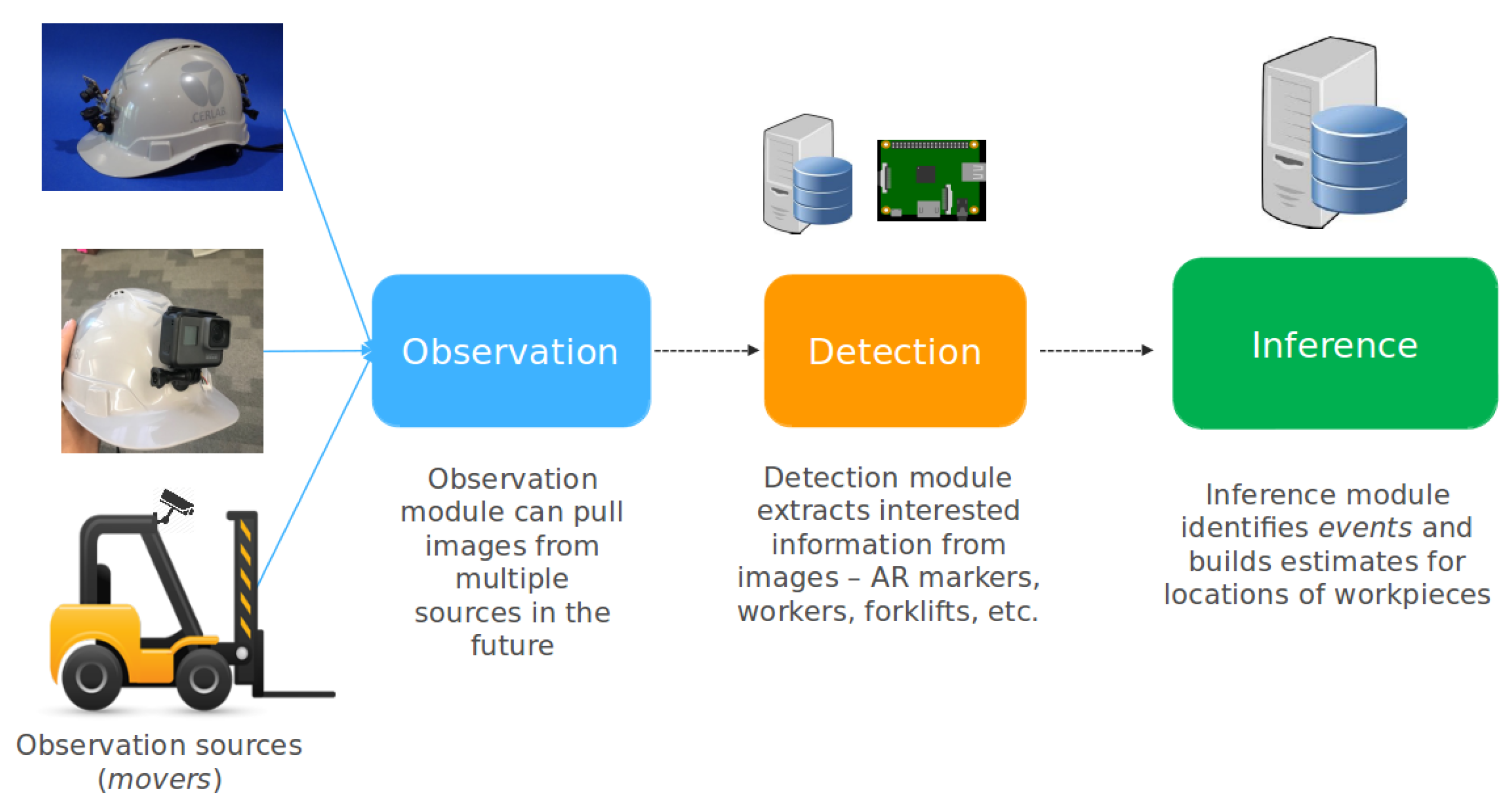
- Observes and logs location and timestamps of workpieces from images through a network of observers;
- Identifies, weighs and logs possible interaction of a workpiece with other workpieces into a graph; and
- Identifies dependencies between workpieces, through a graph, that could have stemmed from events to propose search locations for missing workpieces.
2. Related Work
3. System Architecture
4. Identifying Events and Building Location Estimates Using Graphs
- The stacking of one workpiece on top of another
- Movement of the stack from one location onto another stack
- Splitting of a stack into multiple stacks and moving them to other locations and stacks
- Go through all movers/workpieces that were observed within the vicinity of its last known position.
- Rank or weigh the list of movers that could have taken the workpiece based on the duration and proximity of interaction or lingering. The longer is the duration and closer is the proximity, more likely it is that they interacted with the workpiece.
- Follow the suspect list of movers thereon and identify a list of locations at which the workpiece could have been dropped off.
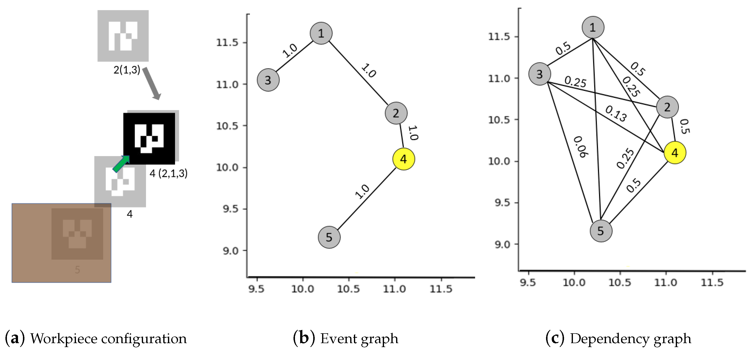
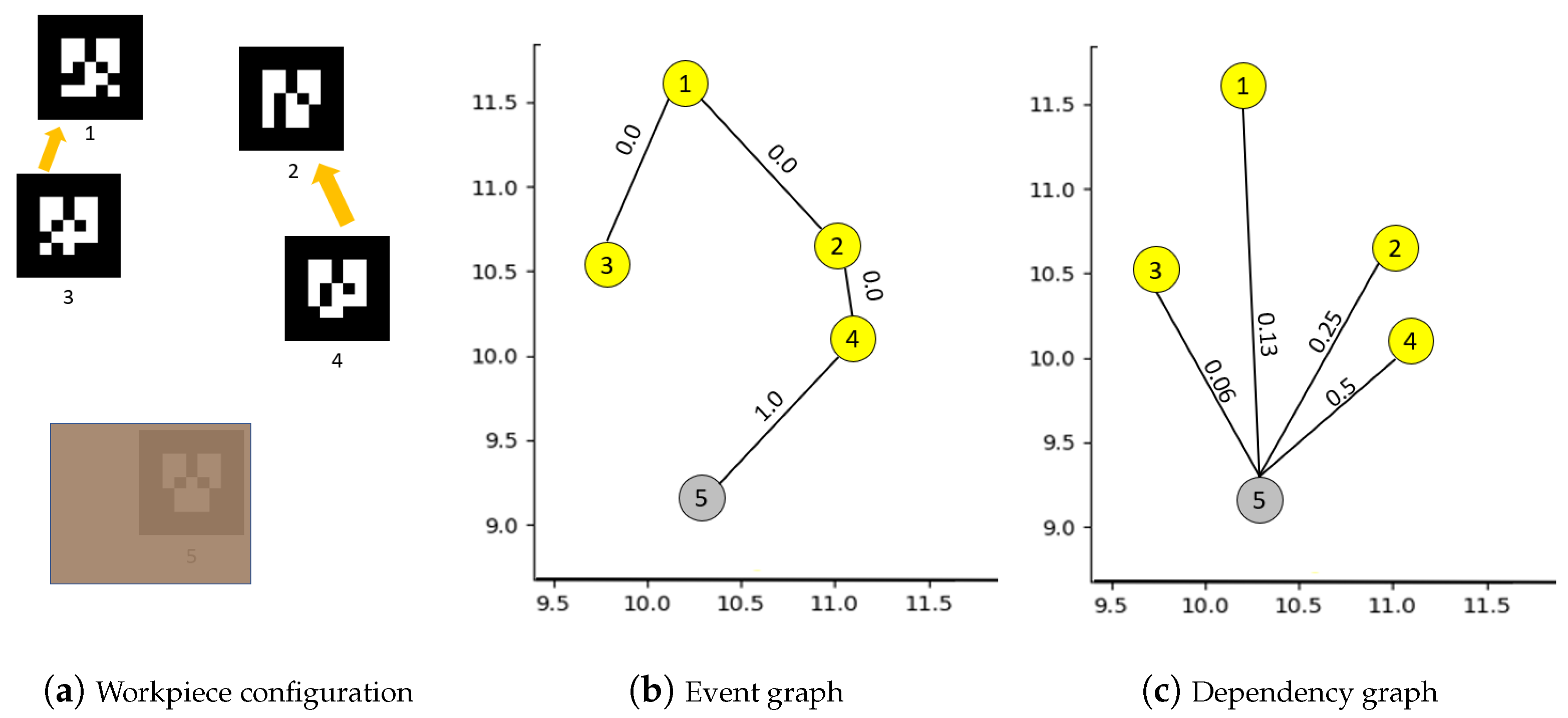
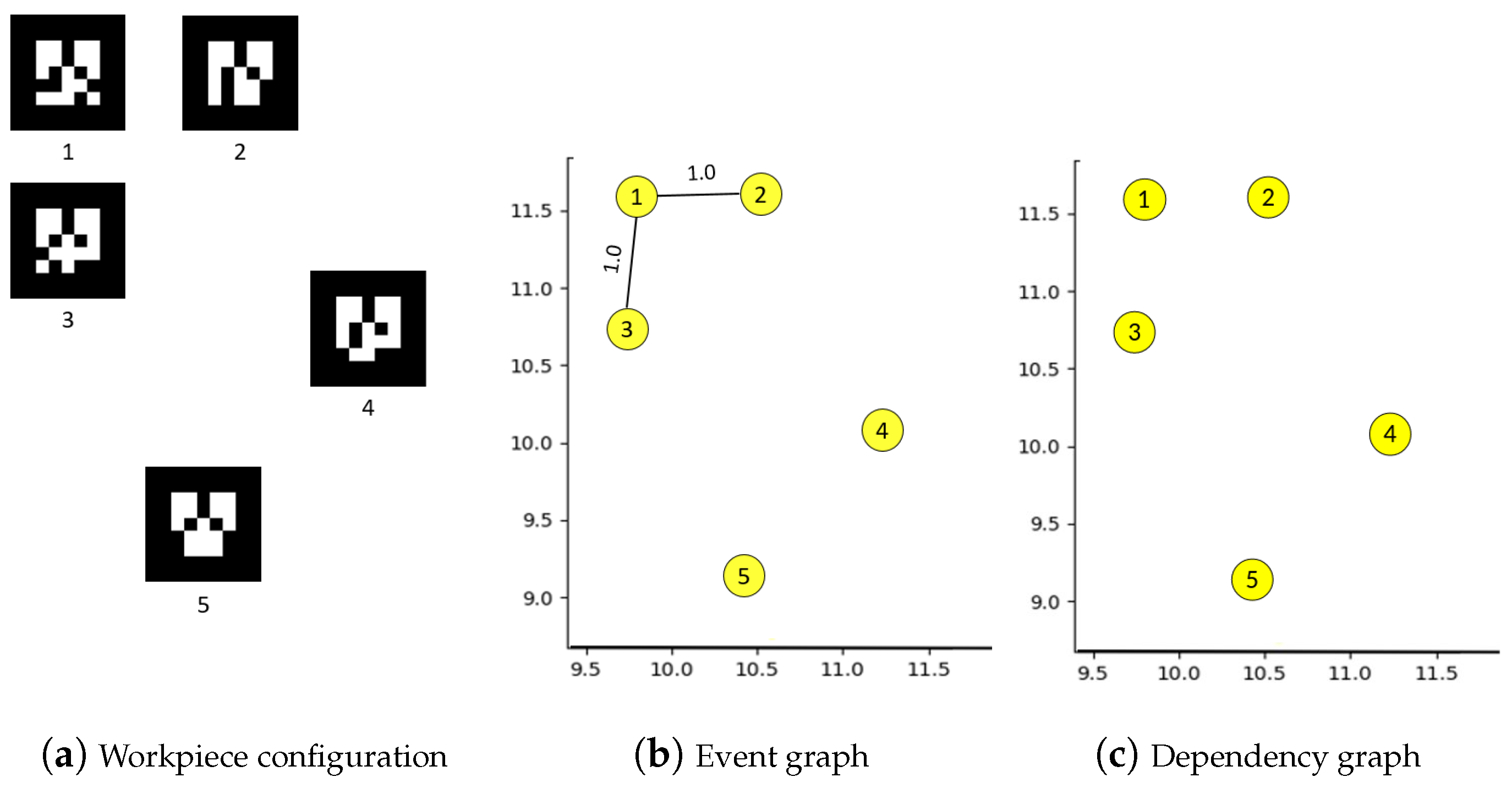
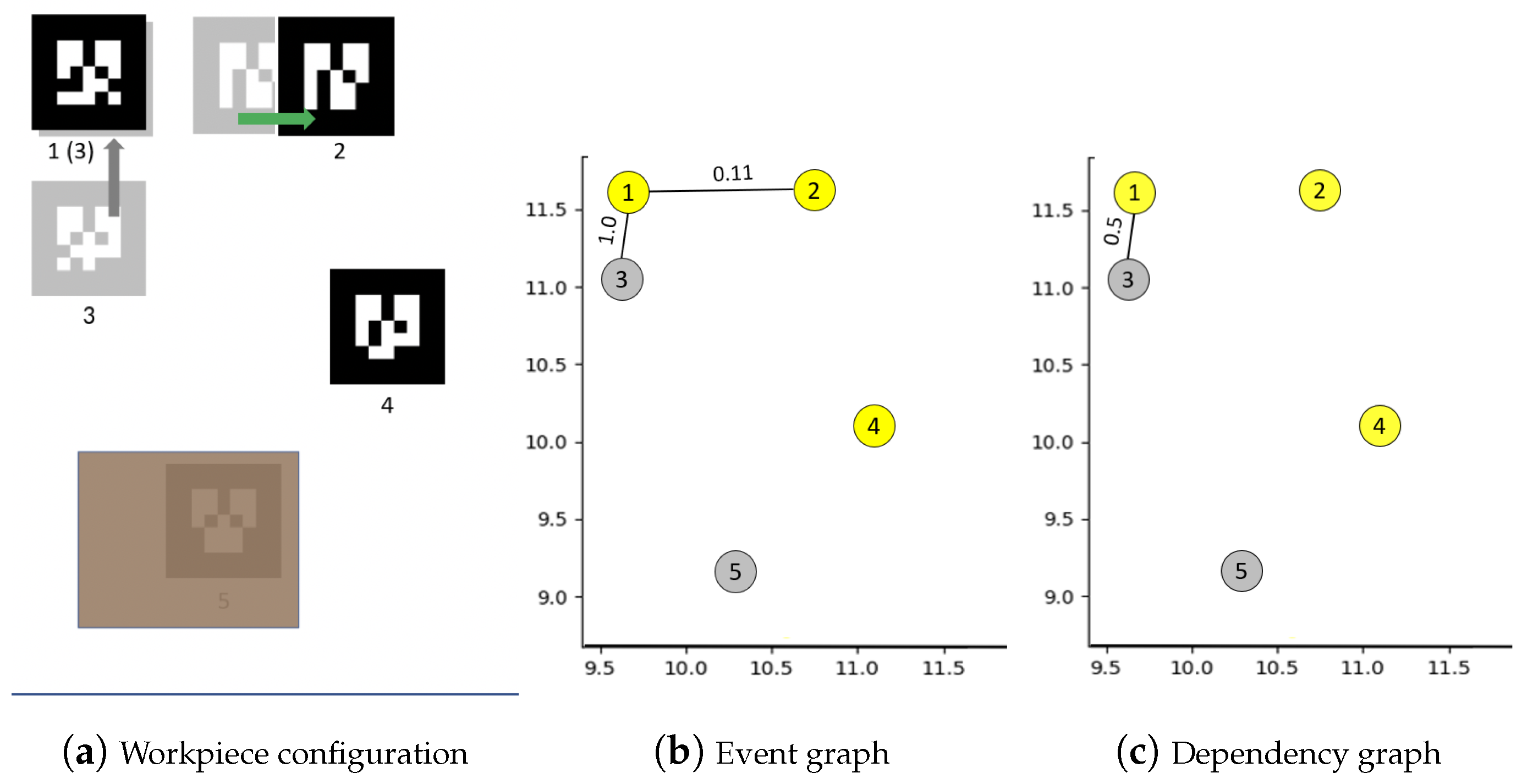
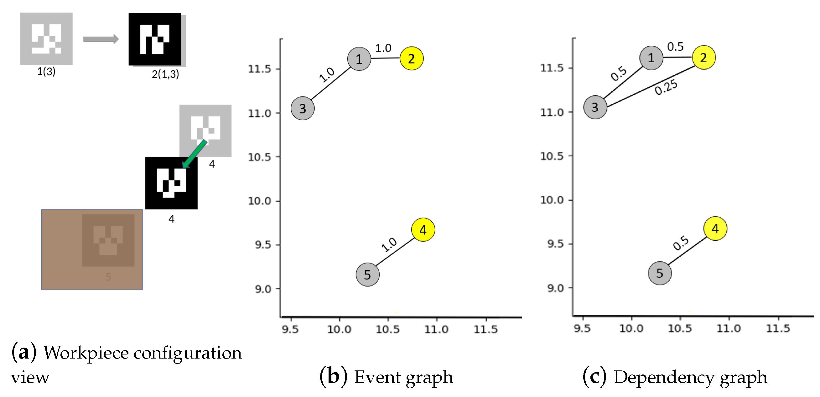
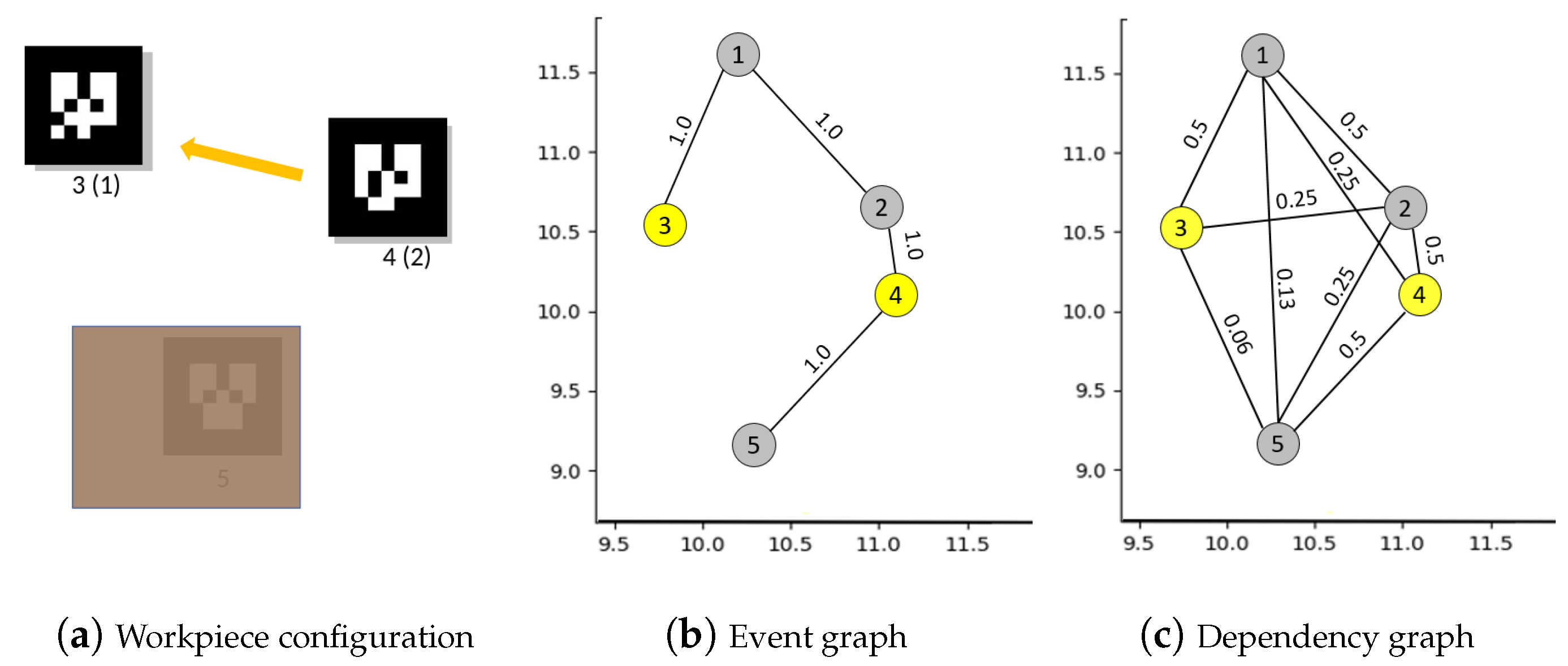
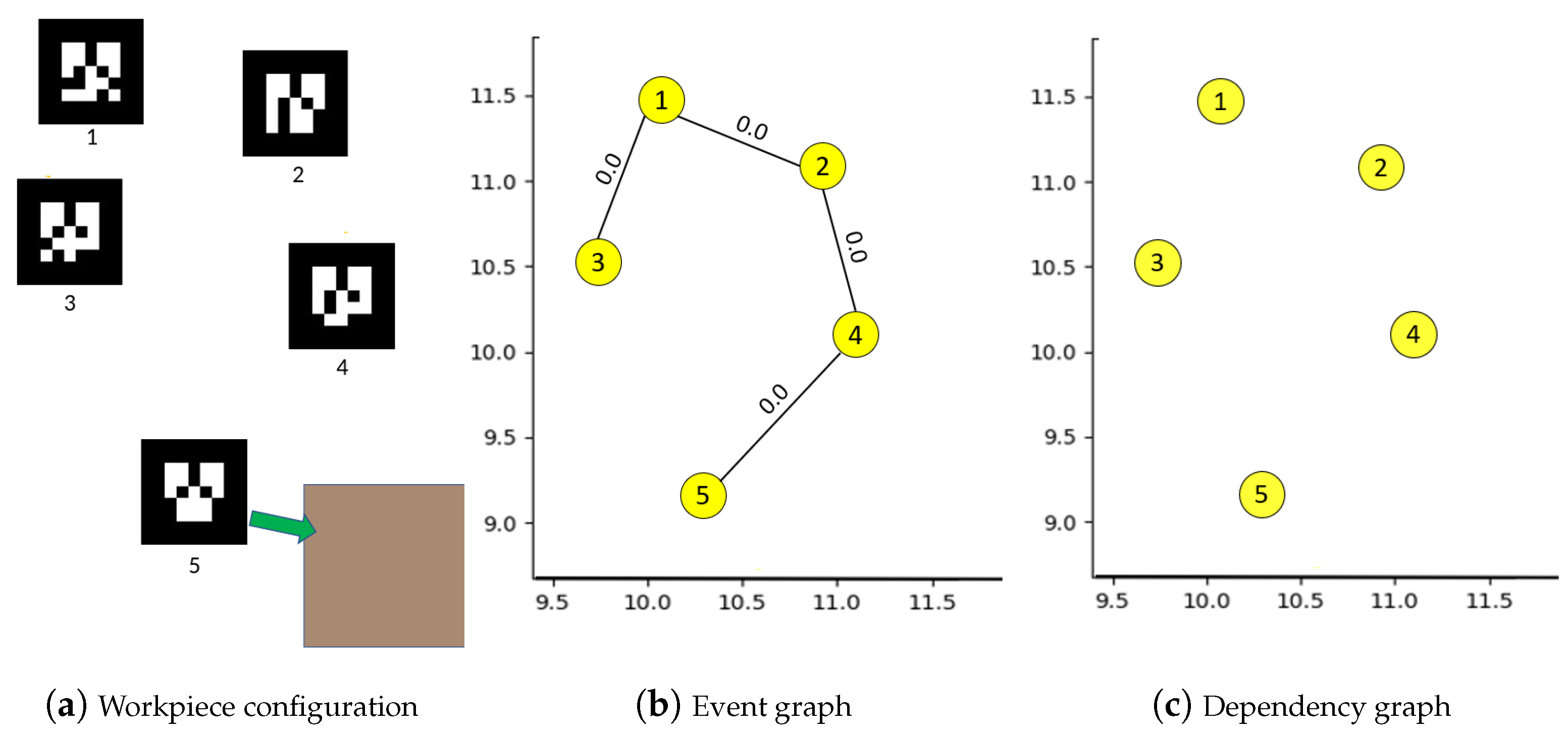
4.1. Building Graph of Events between Workpieces
| is the function parameter for h(.) | |
| represents time | |
| is the edge weight between and at time t in the graph . |
| Algorithm 1: Building event graph . |
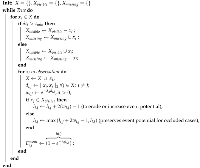 |
| Elapsed time since last observation for workpiece i | |
| User defined time threshold to set the state of a workpiece as missing. This is set to two seconds in our experiments. | |
| Rate parameter for an exponential distribution to decide weight decay within a workpiece’s neighborhood (user set parameter). Smaller values of has wider neighborhoods with softer weights translating to slower rate of increase in the linger counter within the neighborhood. Higher values have smaller neighborhoods with sharp weights within, translating to sharp increase in linger counter when workpieces are within the tight neighborhood. | |
| Weight attributed to proximity factor modeled as an exponential decay for lower values at larger distances between workpieces | |
| Linger counter to increase or erode potential for an event with time. Longer a workpiece is observed within proximity (lingers), higher the value. Range is clipped as to keep the value bounded. | |
| Rate parameter to convert cumulated linger values to a probabilistic estimate through an exponential cumulative distribution function. Smaller values for translates slower rate of increase in event potential whereas a higher value produces a higher rate of increase. The values are determined by the user depending on the workpiece movement character. Note that rate at which the event potential reaches 1.0 can be controlled with both and |
- Present and visible;
- Present but occluded in its last seen position; or
- Moved to another position but still occluded due to event(s).
- We lose line-of-sight for all workpieces that get stacked upon.
- The workpiece on top of the stack is the only workpiece that can be directly observed and tracked.
- A stack might get dispersed, shuffled or split into other stacks while not having a line-of-sight for all its members.
| Algorithm 2: Building dependency graph . |
 |
| Shortest path (based on edge weights) between nodes i and k in . | |
| Distance in terms of node separation between i and k. | |
| Penalty factor for separation. |
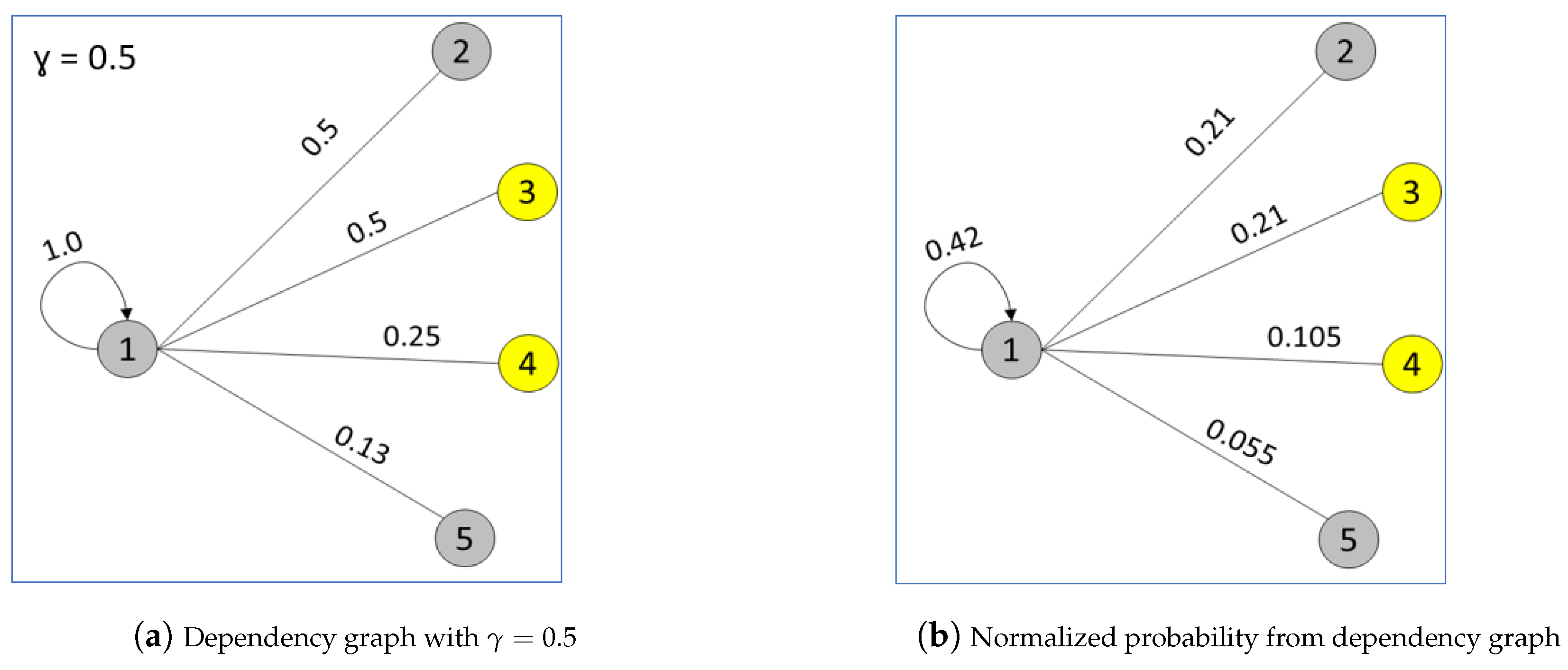
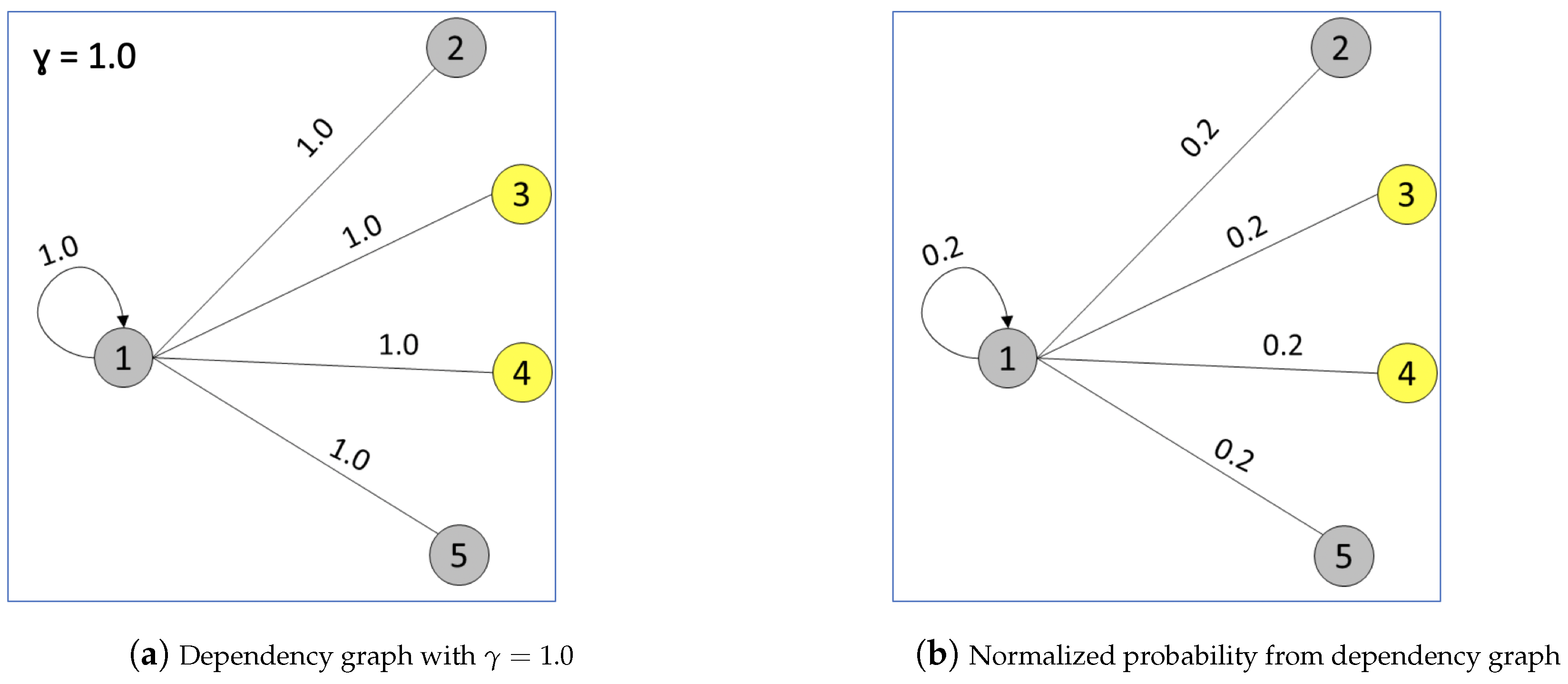
4.2. Native Mechanisms in Our Graph Model
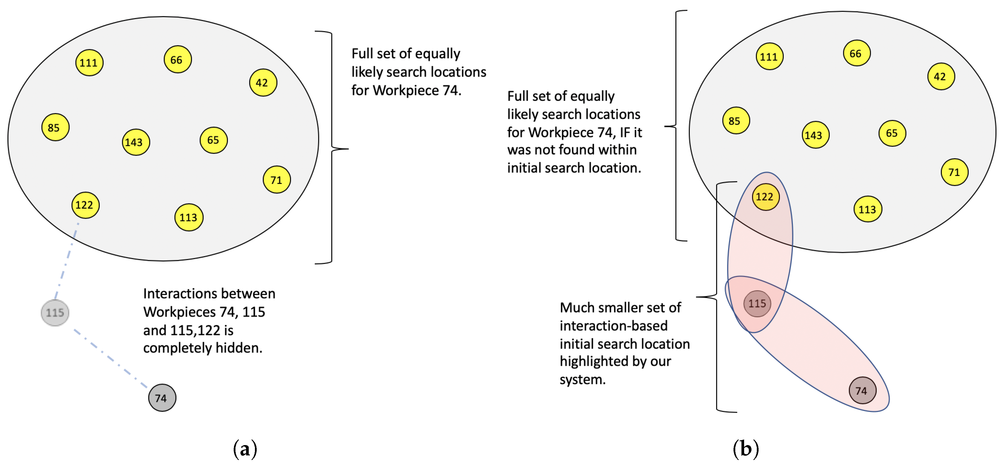
5. Experiments and Results
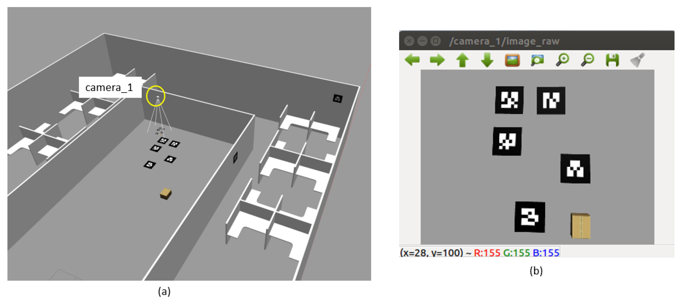
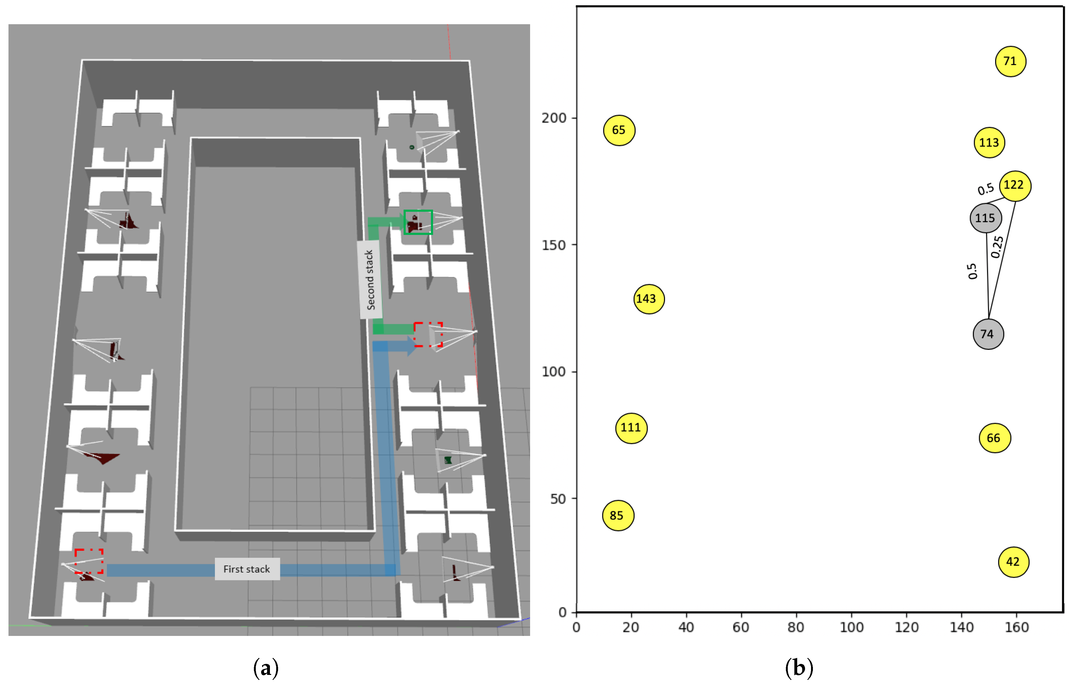
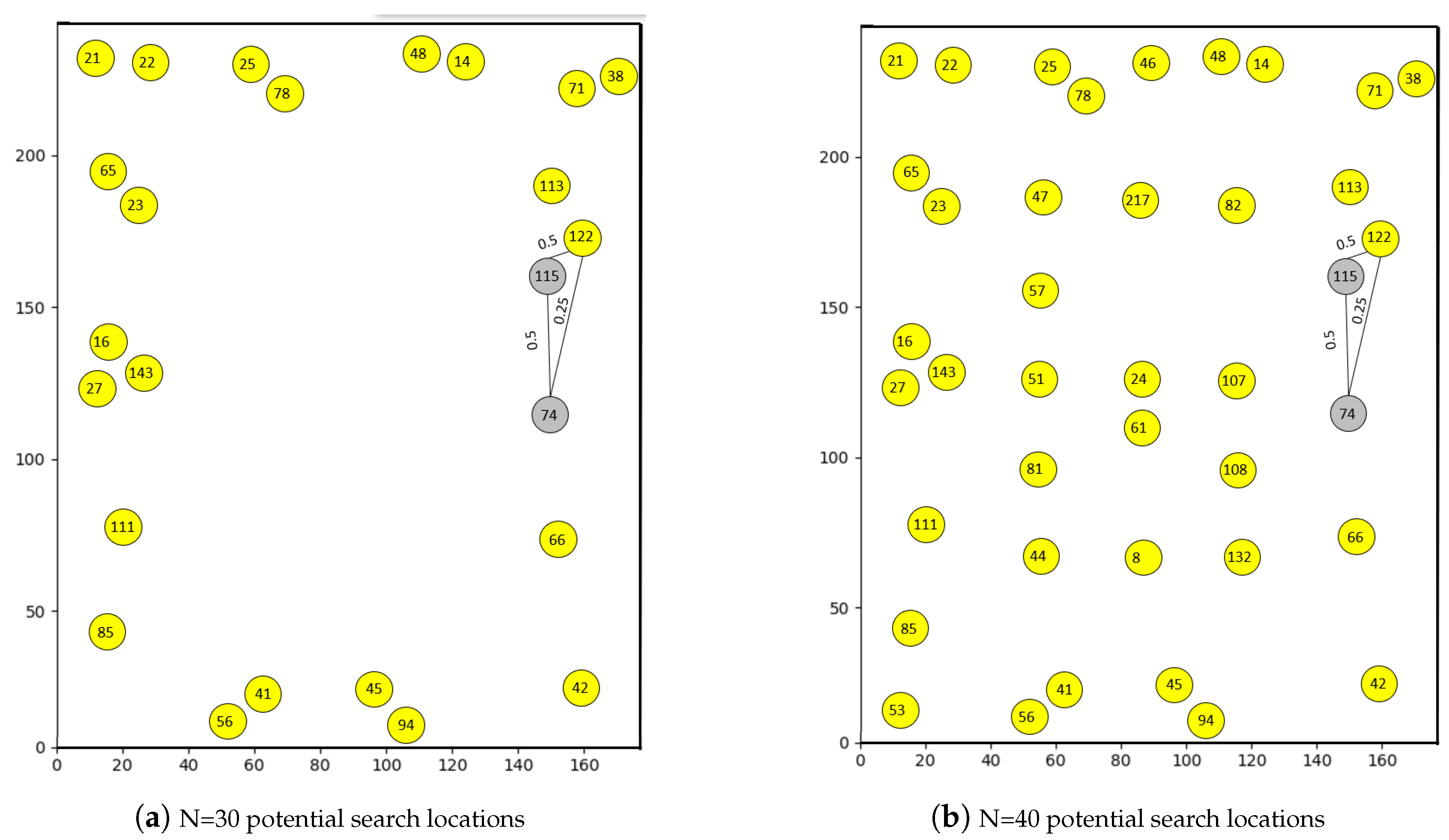
5.1. Simulation Based Experiments
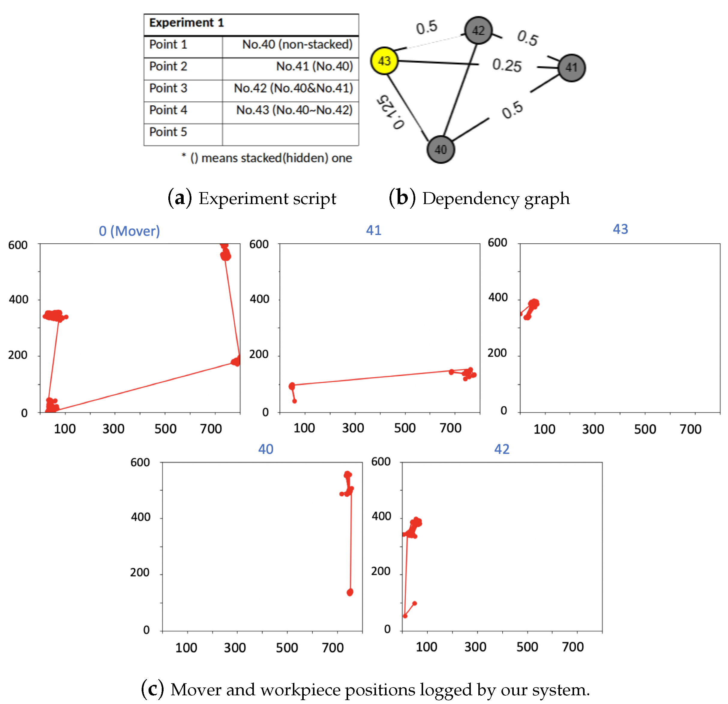
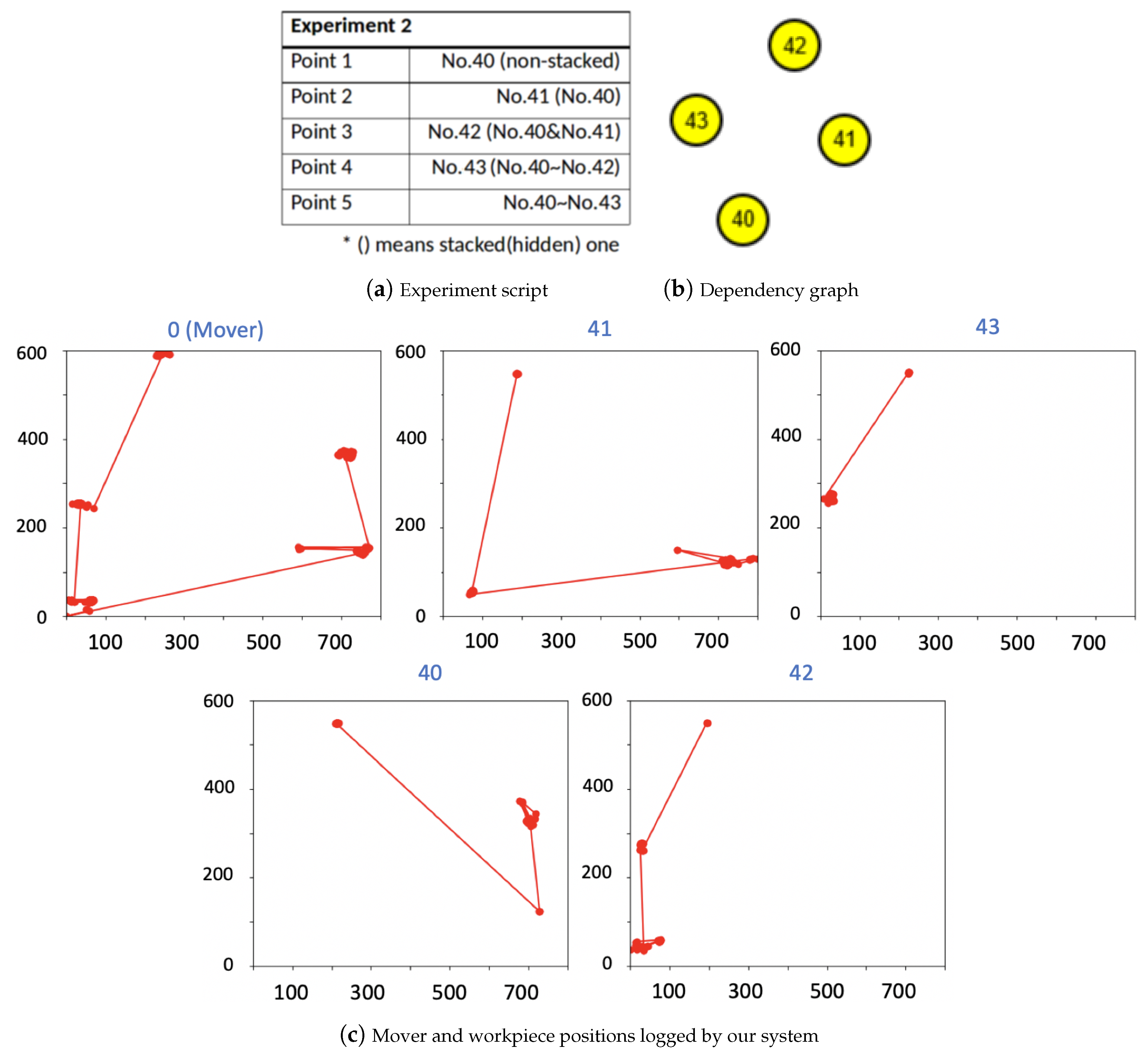
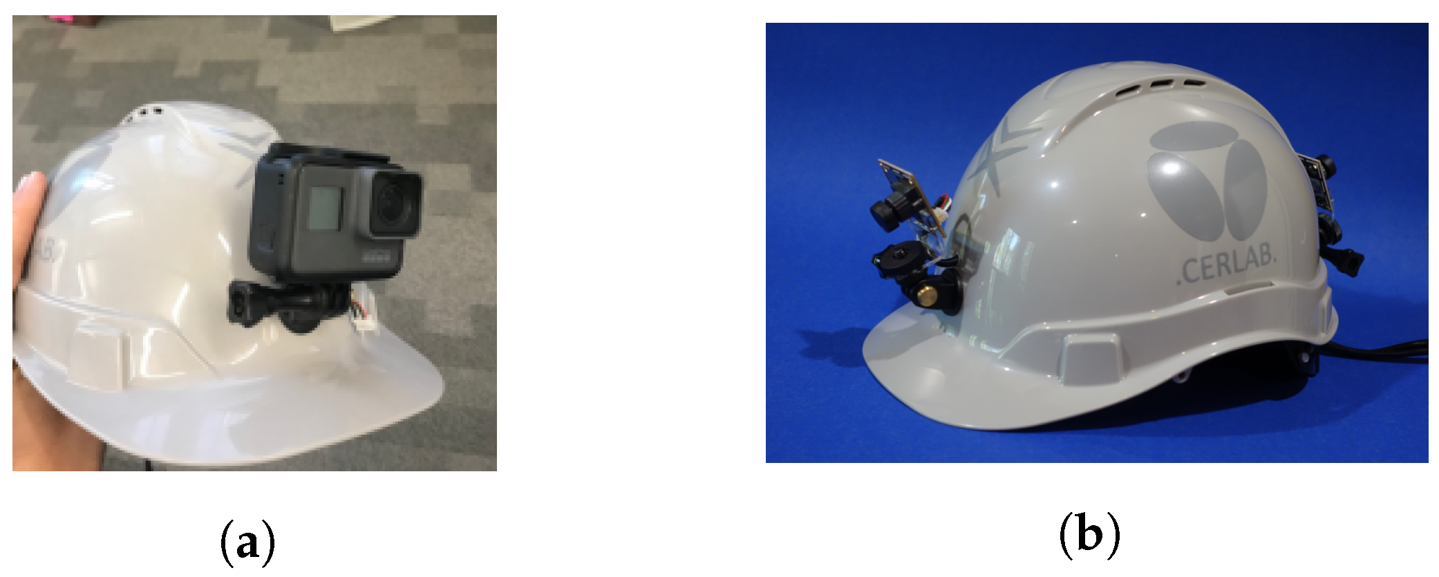
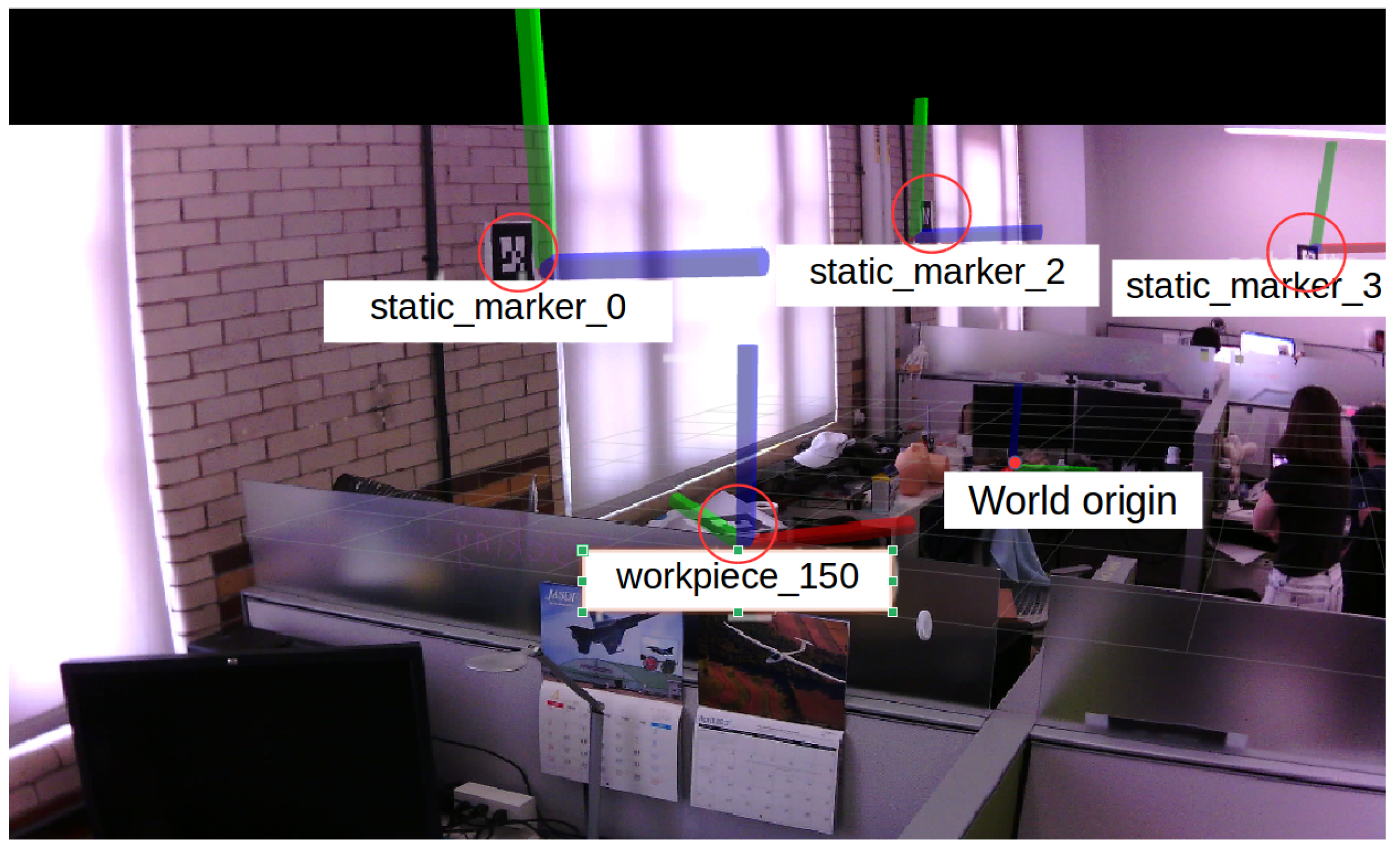
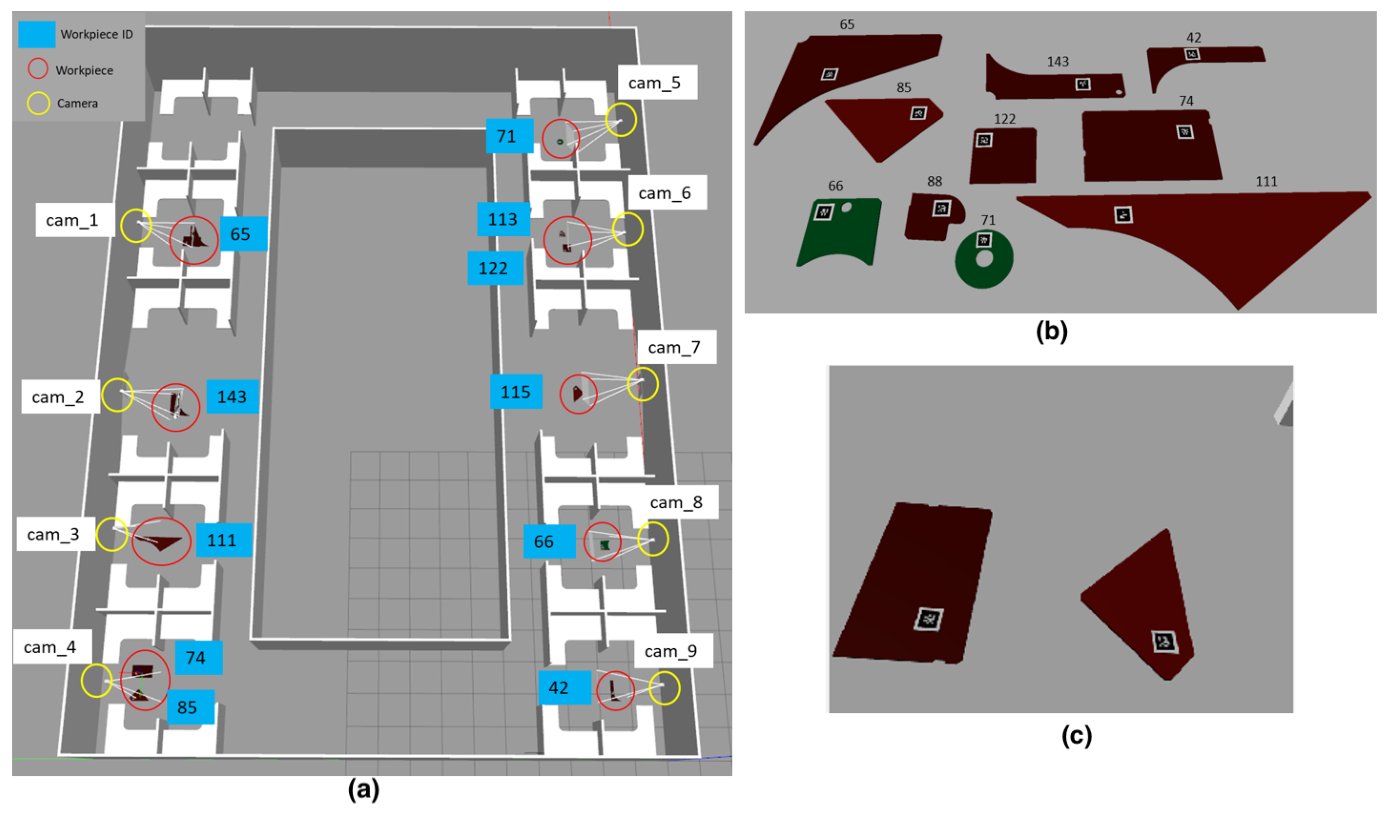
5.2. Real World Experiments
6. Conclusions
Author Contributions
Funding
Conflicts of Interest
References
- Kasim, N.; Liwan, S.R.; Shamsuddin, A.; Zainal, R.; Kamaruddin, N.C. Improving on-site materials tracking for inventory management in construction projects. In Proceedings of the International Conference of Technology Management, Business and Entrepreneurship, Melaka, Malaysia, 18–19 December 2012; pp. 2008–2013. [Google Scholar]
- Dakhli, Z.; Lafhaj, Z. Considering materials management in construction: An exploratory study. Logistics 2018, 2, 7. [Google Scholar] [CrossRef]
- Navon, R.; Berkovich, O. An automated model for materials management and control. Constr. Manag. Econ. 2006, 24, 635–646. [Google Scholar] [CrossRef]
- Grau, D.; Caldas, C.H.; Haas, C.T.; Goodrum, P.M.; Gong, J. Assessing the impact of materials tracking technologies on construction craft productivity. Autom. Constr. 2009, 18, 903–911. [Google Scholar] [CrossRef]
- Bell, L.C.; Stukhart, G. Costs and benefits of materials management systems. J. Constr. Eng. Manag. 1987, 113, 222–234. [Google Scholar] [CrossRef]
- Harrington, T.C.; Lambert, D.M.; Vance, M.P. Implementing an effective inventory management system. Int. J. Phys. Distrib. Logist. Manag. 1990, 20, 17–23. [Google Scholar] [CrossRef]
- Sardroud, J.M.; Limbachiya, M.; Saremi, A. Ubiquitous tracking and locating of construction resource using GIS and RFID. In Proceedings of the 6th GIS Conference and Exhibition (GIS 88), Tehran, Iran, 6 January 2010. [Google Scholar]
- Jang, W.S.; Skibniewski, M.J. A wireless network system for automated tracking of construction materials on project sites. J. Civ. Eng. Manag. 2008, 14, 11–19. [Google Scholar] [CrossRef]
- Lukowicz, P.; Timm-Giel, A.; Lawo, M.; Herzog, O. Wearit@ work: Toward real-world industrial wearable computing. IEEE Pervasive Comput. 2007, 6, 8–13. [Google Scholar] [CrossRef]
- Zhong, R.Y.; Peng, Y.; Xue, F.; Fang, J.; Zou, W.; Luo, H.; Ng, S.T.; Lu, W.; Shen, G.Q.; Huang, G.Q. Prefabricated construction enabled by the Internet-of-Things. Autom. Constr. 2017, 76, 59–70. [Google Scholar] [CrossRef]
- Teizer, J. Status quo and open challenges in vision-based sensing and tracking of temporary resources on infrastructure construction sites. Adv. Eng. Inform. 2015, 29, 225–238. [Google Scholar] [CrossRef]
- Fang, Q.; Li, H.; Luo, X.; Ding, L.; Rose, T.M.; An, W.; Yu, Y. A deep learning-based method for detecting non-certified work on construction sites. Adv. Eng. Inform. 2018, 35, 56–68. [Google Scholar] [CrossRef]
- Teizer, J.; Vela, P.A. Personnel tracking on construction sites using video cameras. Adv. Eng. Inform. 2009, 23, 452–462. [Google Scholar] [CrossRef]
- Salonen, T.; Sääski, J.; Hakkarainen, M.; Kannetis, T.; Perakakis, M.; Siltanen, S.; Potamianos, A.; Korkalo, O.; Woodward, C. Demonstration of assembly work using augmented reality. In Proceedings of the 6th ACM international conference on Image and video retrieval, Amsterdam, The Netherlands, 9–11 July 2007; ACM: New York, NY, USA, 2007; pp. 120–123. [Google Scholar]
- Aleksy, M.; Vartiainen, E.; Domova, V.; Naedele, M. Augmented reality for improved service delivery. In Proceedings of the 2014 IEEE 28th International Conference on Advanced Information Networking and Applications (AINA), Victoria, BC, Canada, 13–16 May 2014; IEEE: Piscataway, NJ, USA, 2014; pp. 382–389. [Google Scholar]
- Mueller, E.T. Commonsense Reasoning: An Event Calculus Based Approach; Morgan Kaufmann: Burlington, MA, USA, 2014. [Google Scholar]
- Xu, Y.; Qin, L.; Liu, X.; Xie, J.; Zhu, S.C. A causal and-or graph model for visibility fluent reasoning in tracking interacting objects. In Proceedings of the IEEE Conference on Computer Vision and Pattern Recognition, Salt Lake City, UT, USA, 18–22 June 2018; pp. 2178–2187. [Google Scholar]
- Fire, A.; Zhu, S.C. Inferring Hidden Statuses and Actions in Video by Causal Reasoning. In Proceedings of the IEEE Conference on Computer Vision and Pattern Recognition Workshops, Honolulu, HI, USA, 21–26 July 2017; pp. 48–56. [Google Scholar]
- Quigley, M.; Conley, K.; Gerkey, B.P.; Faust, J.; Foote, T.; Leibs, J.; Wheeler, R.; Ng, A.Y. ROS: An open-source Robot Operating System. In Proceedings of the ICRA Workshop on Open Source Software, Kobe, Japan, 12–17 May 2009. [Google Scholar]
- Neikum, S. ROS, Ar-Track-Alvar Package. Available online: http://wiki.ros.org/ar_track_alvar (accessed on 7 March 2019).
- Chae, S.; Seo, J.; Yang, Y.; Han, T.D. ColorCodeAR: Large identifiable ColorCode-based augmented reality system. In Proceedings of the 2016 IEEE International Conference on Systems, Man, and Cybernetics (SMC), Budapest, Hungary, 9–12 October 2016; IEEE: Piscataway, NJ, USA, 2016; pp. 002598–002602. [Google Scholar]
- Pentenrieder, K.; Meier, P.; Klinker, G. Analysis of tracking accuracy for single-camera square-marker-based tracking. In Proceedings of the Dritter Workshop Virtuelle und Erweiterte Realitat der GIFachgruppe VR/AR, Koblenz, Germany, 25–26 September 2006. [Google Scholar]
- Wang, J.; Olson, E. AprilTag 2: Efficient and robust fiducial detection. In Proceedings of the 2016 IEEE/RSJ International Conference on Intelligent Robots and Systems (IROS), Daejeon, Korea, 9–14 October 2016; IEEE: Piscataway, NJ, USA, 2016; pp. 4193–4198. [Google Scholar]
- Barbehenn, M. A note on the complexity of Dijkstra’s algorithm for graphs with weighted vertices. IEEE Trans. Comput. 1998, 47, 263. [Google Scholar] [CrossRef]
- Gazebo, Robot Simulation Made Easy. Available online: http://gazebosim.org (accessed on 7 March 2019).
- Mur-Artal, R.; Tardós, J.D. Orb-slam2: An open-source slam system for monocular, stereo, and rgb-d cameras. IEEE Trans. Robot. 2017, 33, 1255–1262. [Google Scholar] [CrossRef]
- Redmon, J.; Divvala, S.; Girshick, R.; Farhadi, A. You only look once: Unified, real-time object detection. In Proceedings of the IEEE Conference on Computer Vision and Pattern Recognition, Las Vegas, NV, USA, 26 June–1 July 2016; pp. 779–788. [Google Scholar]


| Expected Number of Search Locations | ||||
|---|---|---|---|---|
| Stacking | N | Our System | Guess | Reduced Search Locations |
| First stack | 5 | 1 | 3 | 2 |
| First stack | 11 | 1 | 6 | 5 |
| First stack | 50 | 1 | 25.5 | 2 |
| Second stack | 5 | 2 | 3 | 1 |
| Second stack | 11 | 2 | 6 | 4 |
| Second stack | 50 | 2 | 25.5 | 23 |
© 2019 by the authors. Licensee MDPI, Basel, Switzerland. This article is an open access article distributed under the terms and conditions of the Creative Commons Attribution (CC BY) license (http://creativecommons.org/licenses/by/4.0/).
Share and Cite
Rajaraman, M.; Philen, G.; Shimada, K. Tracking Tagged Inventory in Unstructured Environments through Probabilistic Dependency Graphs. Logistics 2019, 3, 21. https://doi.org/10.3390/logistics3040021
Rajaraman M, Philen G, Shimada K. Tracking Tagged Inventory in Unstructured Environments through Probabilistic Dependency Graphs. Logistics. 2019; 3(4):21. https://doi.org/10.3390/logistics3040021
Chicago/Turabian StyleRajaraman, Mabaran, Glenn Philen, and Kenji Shimada. 2019. "Tracking Tagged Inventory in Unstructured Environments through Probabilistic Dependency Graphs" Logistics 3, no. 4: 21. https://doi.org/10.3390/logistics3040021
APA StyleRajaraman, M., Philen, G., & Shimada, K. (2019). Tracking Tagged Inventory in Unstructured Environments through Probabilistic Dependency Graphs. Logistics, 3(4), 21. https://doi.org/10.3390/logistics3040021