Heuristics Algorithms for a Heterogeneous Fleets VRP with Excessive Demand for the Vehicle at the Pickup Points, and the Longest Traveling Time Constraint: A Case Study in Prasitsuksa Songkloe, Ubonratchathani Thailand

Abstract

This paper presents a methodology to solve a special case of the vehicle routing problem (VRP) called the heterogeneous fleets VRP with excessive demand of the vehicle at the pickup points, and the longest time constraint (HFVRP-EXDE-LTC). We developed two metaheuristics—a differential evolution (DE) algorithm and an adaptive large neighborhood search (ALNS)—to solve the problem. These two proposed methods have been designed to effectively solve a special case of VRP. From the computational results, we can see that the proposed heuristics outperformed the best practices that are currently in use. The DE yielded a 9.78% lower cost than that of the current practice (757,250 baht per year), while ALNS generated a 10.89% (906,750 baht per year) lower cost than that of current practice. Comparing the proposed heuristics, ALNS achieved a 1.01% lower cost than that of DE, as ALNS had a better mechanism that was designed to escape from the local optimal.

1. Introduction

In the modern world, technology plays an essential role in business management. One of the main reasons why many companies are poorly managed is because they do not utilize software effectively to manage their business operations. Regarding transportation, an increasing number of companies rely on commercial software to reduce the cost of transportation, as transport prices have increased exponentially over the decades (in Thailand, the logistic cost is currently 14% of the GDP (gross domestic product)). Despite the use of commercial software to attempt to reduce costs, this software is only applicable to certain businesses, as not all businesses have the same transportation needs. Many businesses that utilize commercial software that does not satisfy their business needs often underperform. Therefore, in order for businesses to perform effectively and efficiently, customized software can be integrated into the core of their business plan.

The process of software design comprises seven core steps. These include: (1) software identification and selection; (2) software initiating and planning; (3) analysis; (4) logical design; (5) physical design; (6) system implementation; and (7) system maintenance. The first four steps require the identification of the user’s needs and the discovery of effective solutions to construct a plan for an operative software that will be designed in the latter steps.

This research aims to find effective algorithms to solve a special case of the vehicle routing problem (VRP) (the first four steps of software design). This customized VRP has many attributes and functions in addition to already published algorithms or commercial software. The proposed case study is to design a customized operational software for a school bus pickup and delivery system with an annual budget of 10,619,250 baht to operate the entire system.

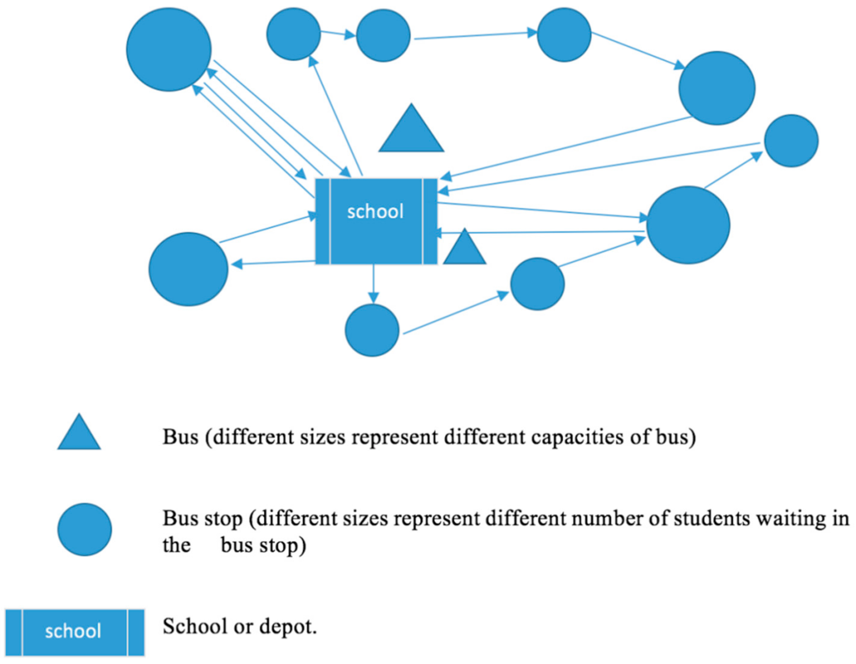
A school bus pickup and delivery system may seem to be an unproblematic system to manage. However, it is a complex system because it consists of many variables that need to be taken into account. Firstly, students need to be picked up from their nearest bus stops and delivered to school on time. Secondly, distances between students’ houses to bus stops must be of acceptable walking distances. Thirdly, the number of students assigned to a bus must not exceed its capacity. Lastly, the number of students assigned to a bus stop must not exceed its capacity. Once these variables are integrated into the simple VRP, the system becomes more complicated. Overall, the core rules that the system must satisfy are: (1) multiple fleets’ VRP; (2) exceed capacity at some pickup points (a bus stop can be visited by more than once); (3) longest time constraints; and (4) capacitated VRP. Despite these core rules, the service of the school bus needs to be good enough so that there would be no complaints from the parents.

The classical VRP was first introduced by Dantzig and Ramser [1] in the article “Truck Dispatching Problem”. Using a specific customized algorithm, they determined how a fleet of homogeneous trucks could serve the demand of multiple gas stations from a central hub while minimizing the distance traveled. Current VRP models are immensely different from the one introduced by Dantzig and Ramser [1], and Lenstra and Rinnooy [2] asserted that VRP is an NP-hard problem.

Various types of VRP have been consecutively proposed after Dantzig and Ramser [1], such as a VRP with time windows, a VRP with heterogeneous fleets, or the multiple depot heterogeneous vehicle routing problem with time windows [3,4,5]. The studies by Braekers et al. [6] and Braelers et al. [7] give an overview of a scenario and its associated physical characteristics problems, extending the basic incapacitated VRPs that have been considered most often in review articles.

VRP is one type of network and communication problem; in the new era, many applications of network problems have been studied. The objective function can have a single objective, multiple cost terms, or multiobjectives. Tsiropoulou et al. [8] and Tsiropoulou et al. [9] presented a joint interest in the physical and energy-aware clustering and resource management framework of the of machine-to-machine (M2M)-driven Internet of Things (IoT). Lin and Gerla [10] described a self-organizing, multi-hop, mobile radio network that relies on a code-division access scheme for multimedia support. Wu et al. presented a good survey of the communication area [11]. The reader can find excellent reviews of vehicle routing problems in Kim et al. [12], Karakatič and Podgorelec [13], Gupta and Saini [14], and Braekers et al. [6].

The case study, the school bus pickup and delivery problem, is one special case of VRP. This problem focuses on the heterogeneous fleets’ vehicle routing problem excessive demand of the vehicle at the pickup point, and the longest time constraint (HFVRP-EXDE-LTC), which is not mentioned in the previous literature.

There have been many publications that have proposed methods to solve this problem, such as tabu search [15], the evolutionary algorithm [16], and the genetics algorithm [17,18]. Differential evolution (DE) algorithms are widely used to solve many problems, including VRPs such as Pitakaso [19], Pitakaso and Sethanan [20], López et al. [21], Liao et al. [22], and Liao et al. [23]. Hou et al. [24] presented a discrete DE with modified process operators. Dechampai et al. [25], Akkararungruangkul, and Kaewman [26] proposed a DE to solve the capacitated VRP with the flexibility of mixing pickup and delivery services and the maximum duration of a route in the poultry industry. Boon et al. [27] uses DE to solve the capacitated vehicle routing problem by combining it with local search techniques. The DE is more effective if the local search is included, but it increases the computational time [28]. The DE is modified by adding some more processes to the original version such as a recombination process, reborn process, and reincarnation process to get better solutions [29,30,31,32,33]. These processes can improve the solution quality of the original DE due to it enhancing the search capability of the original system. From the computational result of the proposed DE, it outperformed all of the other heuristics while solving the same problem. Thus, DE was one of the heuristics selected to solve the case study in this article.

The adaptive large neighborhood search (ALNS) was introduced by Shaw [34] for the capacitated vehicle routing problem (CVRP). Later on, ALNS was widely used in various problems, including Aksen [35], which was a study of a selective and periodic inventory routing problem (SPIRP). Azi et al. [36] proposed an ALNS for solving a VRP with multiple routes (VRPM). Emec et al. [37] presented new removal, insertion, and vendor selection allocation mechanisms. Ribeiro and Laporte [38] proposed an ALNS for solving the cumulative capacitated vehicle routing problem (CCVRP). Hemmelmayr et al. [39] proposed an ALNS heuristic for the two-echelon vehicle routing problem (2E-VRP). The results of ALNS when applied to all of the problems outperformed the previously proposed algorithms, and thus, the ALNS was the second heuristic that we selected to solve the presented case study.

From the literature review, the DE has been proposed to solve various types of combinatorial problems, and it outperforms all of the previous algorithms due to it being fast and effective, as shown in Pitakaso [19], Pitakaso and Sethanan [20], López et al. [21], Liao et al. [22], Liao et al. [23], and Hou et al. [24]. ALNS has been developed to solve mostly network problems such as VRP, and it is very flexible when it comes to designing algorithms to solve the proposed problems, as shown in Aksen [34] and Emec et al. [37]. The proposed problem is the heterogeneous fleets vehicle routing problem with excessive demand of the vehicle at the pickup point, and the longest time constraint (HFVRP-EXDE-LTC), whereby the new, modified DE algorithm and ALNS were designed to solve this new class of VRP. We select these two algorithms due to their flexibility, easy modification, and use of only a few parameters. Moreover, these two metaheuristics have been successfully used in many combinatorial optimizations.

This paper covers five sections. Section 1 is the introduction. Section 2 is the definition of the problem and the best practices procedure that is currently used. The proposed heuristics are shown in Section 3, while the computational results and the conclusion and outlook are shown in Section 4 and Section 5, respectively.

2. Problem Definition and the Best Practices Procedure

2.1. Problem Definition

The proposed problem is a special case of VRP that has the following attributes:

(1)

The decision problem is to determine the route(s)of the vehicles to pick students up from bus stops to minimize the total traveling cost and rental cost of the vehicles.

(2)

The demand at each pickup point is known, and it is possible for the demand to exceed the capacity of the various types of vehicles.

(3)

One vehicle can pick students up from more than one route, which can be the same bus stop if there are still some students left at that bus stop after previous vehicle visits due to the limited capacity of the bus.

(4)

There is a travel time limitation to complete a journey, since the school needs to start at a planned time every day.

(5)

One pickup point can be visited by more than one vehicle, or

(6)

One pickup point can be visited by the same vehicle that travels more than one time.

(7)

The problem is an asymmetric vehicle routing problem.

The proposed problem is depicted in Figure 1.

2.2. The Current Practice Procedure

The current best practices procedure that the school is using to plan the pickup of students is as follows:

(1)

Select the bus by the capacity of the bus (the biggest bus is elected first and the smallest bus is selected last).

(2)

The bus is sent to the biggest bus stop first. If there are any students remaining at the bus stop, another bus from other bus stops is sent to pick them up.

(3)

The traveling time is calculated, and it has to be within a certain time limit.

Let us consider a scenario. There are six pickup points and each point has 10, 30, 40, 20, 15, or 60 students waiting at that bus stop, respectively. Additionally, there are four buses available (two small and two big), and each bus has a capacity of 40, 40, 60, or 60, respectively. The rental cost of each bus is 1500, 1500, 2000, or 2000 baht per day. The fuel charge is 4.5 baht per kilometer, and the distances between the school (0) and all of the other bus stops are shown in

Table 1. Distances between all of the points (bus stops and school) in the proposed problem (in km), whereby 0 is the school and 1–6 are the bus stops. Please note that this is an asymmetric distance due to one-way roads or the road being blocked because of construction.

	0	1	2	3	4	5	6
0	0	30	13	27	20	23	21
1	8	0	10	16	21	19	12
2	5	27	0	10	26	11	13
3	25	10	23	0	21	9	17
4	6	22	10	8	0	26	14
5	18	16	15	18	27	0	11
6	11	14	22	17	17	5	0

. The traveling time is 40 km per hour, and the maximum time for each route is 1.5 h or 60 km (both ways).

The order of the buses to travel to pick students up are Bus 1, Bus 2, Bus 3, and Bus 4. Bus 1, with a capacity of 60 students, is sent out to pick students up from the biggest bus stop (bus stop6). Therefore, Bus 1 has route 0-6-0 (number of students that are picked up is 60, and it has a traveling time of 33 min). Bus 1 has 27 extra minutes, but if it goes for another round to pick up students at bus stop 3 (the second biggest bus stop), it would not have enough time to come back to the school on time (60 min). Thus, Bus 1 is not used for a second round, and Bus 2 is sent out to pick students up. If we continue until all of the buses are used and all of the students are delivered to the school, we get all of the traveling routes shown in

Table 2. Results of the best practices procedure. From the table, the total traveling distance is 168 km or 339.5 baht (4.5 baht per km). The total cost, which includes the bus rental cost, is 7339.5 baht.

Bus	Route	# Students	Traveling Time
1	0-6-0	60	33
2	0-3-2-0	60	42
	0-2-0	10	18
3	0-4-0	20	26
4	0-5-1-0	25	49

Note: #Student represents number of student.

.

3. Proposed Heuristics

In this section, two metaheuristics are presented. The differential evolution (DE) algorithm and the adaptive large neighborhood search (ALNS) are customized and designed to suit the needs proposed by the problem statements.

3.1. Differential Evolution (DE) Algorithm

The DE algorithm is typically composed of four steps: (1) generate the initial solution; (2) perform the mutation process; (3) perform the recombination process; and (4) perform the selection process. Steps (2)–(4) are iteratively executed until the stopping criteria are achieved. The stopping criteria are the user-defined parameters. These parameters could be time limitations, the number of iterations, or any other predefined behaviors of the algorithm.

3.1.1. Generate Initial Solution

The initial solution is first executed by designing vectors that represent the problem. These vectors are then decoded and used to solve the problem.

To design the DE algorithm for this case study, we needed to define the number of vectors (population). In this scenario, population number was set at four. If there are six bus stops, the vector had a dimension of 1 × 6. The real number in each position of the vector was randomly generated from values of 0 to 1. The resulting randomly generated numbers of all six vectors are shown in

Table 3. Four randomly generated target vectors of the size 1 × 6. From Table 3, all of the values in the position of the vectors are presented. To obtain a solution for this problem, these vectors needed to be decoded, a process which is explained in the following subsection.

	1	2	3	4	5	6
1	0.38	0.42	0.19	0.50	0.21	0.31
2	0.88	0.57	0.71	0.50	0.87	0.68
3	0.08	0.80	0.94	0.33	0.49	0.26
4	0.75	0.12	0.65	0.41	0.85	0.46

. The generated vectors are called target vectors.

Decoding Procedure

The decoding procedure for each vector was performed using the following steps:

(1)

Sort the value in the position of the vector in an ascending order.

(2)

Sort the bus stops according to the value of the position.

(3)

Select the bus to pick students up according to the bus stop order. The selection of the bus applies roulette wheel selection using the following probability formula:

$$p_k=\frac{\frac{C_k}{F_k}+\frac{S_k}{{{\displaystyle \sum }}_{k=1}^K{S}_k}}{{{\displaystyle \sum }}_{k=1}^K\frac{C_k}{F_k}+\frac{S_k}{{{\displaystyle \sum }}_{k=1}^K{S}_k}}$$

(1)

where p_k is the probability of selecting bus k, C_k isthe capacity of bus k, F_k is the fixed rental cost of bus k, and S_k is the current score of bus k, which is iteratively updated. The first iteration S_k is set to 1 for all k.

(4)

If the bus reaches its capacity or reaches the travel time limit, then it must return to the school.

(5)

Repeat steps 3 and 4 until all of the students are picked up.

(6)

Calculate the total cost and update S_k.

Table 3 the execution of steps 1 and 2 for the values in the position of vector 1. The values of the position before and after applying these two steps are shown in

Table 4. Vector before (a) and after (b) applying steps 1 and 2.

(a) Vector 1 before applying steps 1 and 2
1	2	3	4	5	6
0.38	0.42	0.19	0.50	0.21	0.31
(b) Vector 1 after applying steps 1 and 2
3	5	6	1	2	4
0.19	0.21	0.31	0.38	0.42	0.50

a,b, respectively.

Table 4 shows the result of steps 1 and 2, after which, step 3 was performed. The bus that was sent to pick students up was selected using Formula (1). The probabilities of each bus were 0.251, 0.251, 0.249, or 0.249, and the cumulative probabilities were 0.251, 0.502, 0.751, or 1, respectively. Thus, if the random number was 0.43, then Bus 2 was selected. Bus 2 has a capacity of 60, and a rental cost 2000 baht per day.

If Bus 2 was sent to pick students up from the order of the bus stops shown in Table 4, then Bus 2 would go to bus stops 3 and 5, which would take up 55 out of the 60 seats available. However, if Bus 2 picked five students up from bus stop 6 (0-3-5-6(5)-0), then the time used was 58 min, and the capacity used was 60. This effectively maximizes the use of Bus 2.

In the next step, we selected the next bus. If the next bus that was sent out to pick students up at bus stop 6 was Bus 1 (capacity of 60), then there would be five seats remaining in Bus 1, because Bus 2 can only pick up five students from bus stop 6, leaving 55 students at the bus stop, who would board Bus 1. Bus 1 then continued to pick five students up from bus stop 1 before returning to the school. Thus, Bus 1 had the route of 0-6-1(5)-0 and a traveling time of 43 min. Bus 1 cannot complete a second round of pickups, because it will not have enough time for the second round (exceeds 60 min). Thus, the next bus was selected. If Bus 4 was selected, it needed to pick the remaining five students up from bus stop 1. After this, it continued to bus stop 2 to pick 30 students up before returning to the school. The route of Bus 4 was 0-1(5)-2-0. The number of students that were in this bus was 35, and it had a traveling distance of 45 km. If this bus returned to bus stop 4, it would have exceeded the maximum distance allowed. Thus, Bus 4 was not used after the first round. Finally, the last bus (Bus 3) was sent out to pick the remaining 20 students up from bus stop 4, and the bus returned to the school. The time used for this journey was 26 min.

Finally, buses 1, 2, 3, and 4 had the routes 0-6-1(5)-0, 0-3-5-6(5)-0, 0-4-0, and 0-1(5)-2-0, respectively. The total distance was 58 + 43 + 45 + 26 = 172 km, and it had a total cost of 4.50 baht per km. Thus, the total traveling cost was 774 baht and the rental cost was 7000 baht. The total cost was 7774 baht.

3.1.2. Perform the Mutation Process

The next step of DE is to perform a mutation process. The mutation process was applied by using Formula (2). This process randomly selects three vectors out of NP vectors, which are then substituted into Formula (2). The result of the mutation process is a mutant vector:

$$V_{m,n,G}=X_{r1,n,G}+F\left(X_{r2,n,G}-X_{r3,n,G}\right)$$

(2)

where $V_{m,n,G}$ is the mutant vector m with position n iteration G, and Xr_i is the selected target vector r with position n at iteration G. F is the predefined scaling factor.

3.1.3. Perform the Recombination Process

The recombination process is the process that performs the interchange of the values between the mutant vector and the target vector using Formula (3):

$$U_{m,n,G}={\{}_{X m,n,G otherwise}^{Vm,n,G ran{d}_n\le CR }$$

(3)

where $U_{m,n,G}$is the trial vector m with position n at iteration G, and CR is the predefined parameter, which is usually set to 0.6–0.9.

3.1.4. Perform Selection Process

A selection process is a process that selects the next target vector in iteration G + 1. The better vector between the trail vector and the current target vector becomes the G + 1 target vector. This selection process was performed by using Formula (4):

$$X_{m,n,G+1}={{\displaystyle \int }}_{X_{m,n,G}\mathrm{otherwise}}^{U_{m,n,G \mathrm{if}f\left(U_{m,n,G}\right)\le f\left(X_{m,n,G}\right)}}$$

(4)

3.1.5. Updating the Attractiveness of the Buses

In Formula (1), the S_k is iteratively updated for each vector by adding a new score to the bus. The score added to the bus depends on the solution quality that was obtained from having the bus in the solution. The added score is composed of two levels: (1) add six scores for the bus that is the global best result (best solution found so far); and (2) add four scores for the vector’s best result (the trial vector is accepted to be the new target vector). For instance, if at a particular iteration, buses 1, 2, 3, and 4 have an S_k equal to 45, 30, 50, and 16, respectively, then the new global best solution is found to be in vector 1 (compared to all of the other vectors). If only buses 1, 2, and 4 are in the solution of vector 1, then the S_k for buses 1, 2, 3, and 4 will be 51, 36, 50, and 22, respectively. For vector 2, which has the same iteration, if the solution includes buses 1, 3, and 4 for the new vector’s best solution, then the S_k will be updated to 55, 36, 54, and 26, respectively.

Steps 3.1.2–3.1.5 were iteratively executed until the termination condition was satisfied. Generally, the stopping criteria was set to be the number of iterations or the limited computational time. Occasionally though, the end for the search of the best solution or the number of the iterations that gave the best results was fixed, and could be used as the stopping criteria.

3.2. Adaptive Large Neighborhood Search (ALNS)

ALNS is composed of four steps: (1) generate the initial solution; (2) perform the destroy method; (3) perform the repair method; and (4) update all of the parameters, including the global best solution, iteration best solution, and the attractiveness of the destroy and repair methods. Steps (2)–(4) are iteratively executed until the stopping criteria is achieved. The customized ALNS is explained in the following subsection.

3.2.1. Generate the Initial Solution

In this step of ALNS, randomly generated sequences of the bus stops are used to construct the initial sequence. For example, the sequence of the bus stops was randomly generated as {5,2,1,6,4,3}. After the initial sequence was generated, steps (3)–(6) of the decoding method, as explained in Section 3.1.1, were applied to obtain the solution. If in the initial solution, Bus 1 had route 0-5-2-1-0 (the distance (time) used was 52 km, the number of students picked up was 55), then Bus 2 had route 0-6-0 (the distance used was 32 km, the number of students picked up was 60) and Bus 3 had route 0-4-0 (distance used was 26 km (26 km + 32 km = 58 km, which is less than 60 km, which is the maximum time of Bus 2) and the number of students was 20). Finally, Bus 4 picked students up at bus stop 3 and had route 0-3-0 (the distance used was 52 km and the number of students that was in the bus was 40). This solution had a total distance of 162 km (729 baht) and a rental cost of 5500 baht. Thus, the operational total cost was 6229 baht.

3.2.2. Perform the Destroy Method

The destroy method was customized for it to be suitable for the constructive method to get the solution. The bus was selected using Formula (1). The destroy method was designed to deal with the sequences of the bus stops. We designed six types of destroy methods, which are presented in detail below.

3.2.2.1. Remove One Bus Stop from the List (RM)

If the initial sequence (bus stop list) was {5,2,1,6,4,3}, we implied a traveling salesman problem to the list, thus forming the route 0-5-2-1-6-4-3-0. Then, we listed the traveling distance from a bus stop to the current bus stop and called it the distance to bus stop (DB_k). For example, when the k value was 5, the distance from school (0) to bus stop 5 (DB_k) was equal to 23. When value k was 1, 2, 3, 4, 5, and 6, the calculated DB_ks were 5, 16, 8, 17, 23, and 12, respectively. The bus stop that had the highest DB_k value was removed. Thus, bus stop 5 was removed from the list. The new bus stop list was achieved as {2,1,6,4,3}. The removed bus stop was compensated for in the repair method so that we could obtain the complete solution again.

3.2.2.2. Remove Two Bus Stops from the List (RM2)

To perform RM2, we applied a similar method to RM (explained above). The only difference is that in RM2, the first two bus stops with the highest DB_k values were removed, while only one bus stop with the highest DB_k value was removed in RM. Therefore, as seen from the previous calculated DB_k values, bus stops 4 and 5 were removed to produce the new bus stop list of {2,1,6,3}. The removed bus stops were compensated in the repair method.

3.2.2.3. Randomly Remove One Bus Stop from the List (RRM)

RRM involves the random selection of a bus stop. Instead of using distance to remove a bus stop from the list, we randomly selected one bus stop and removed it from the list that was created in the RRM procedure.

3.2.2.4. Randomly Remove Two Bus Stops from the List (RRM2)

This method is similar to the above method (Section 3.2.2.3), but two bus stops were randomly selected and removed from the bus stop list.

3.2.2.5. Remove Bus from the Bus List (RB)

This destroy method starts with forming the bus list. The bus list can be drawn from the best solution bus list. Up to this point, the best solution bus list is shown in the latter example that generated a solution of 6229 baht with a bus list of {1,2,4,3}. In the solution given above, only buses 1, 2, and 3 were used. The removal of the bus was executed by removing the bus that had the lowest S_k score. If the current scores of buses 1, 2, 3, and 4 were 55, 36, 54 and 26, respectively, then Bus 4 would be removed from the list, and the repair method would be performed to obtain the completed solution.

3.2.2.6. Remove 50% of the Buses from the Bus List (0.5 RB)

This destroy method is the same as above (Section 3.2.2.5), but it removes the first 50% (in this example, two buses were removed) of the buses that have the lowest S_k scores. Therefore, following from RB, 0.5 RB removed Bus 2 and Bus 4 from the bus list.

3.2.3. Perform the Repair Method

The repair method was used to rebuild the solution to derive a complete solution. In this article, we present four types of repair methods as follows.

3.2.3.1. Best Insertion (BIn)

The repair method or best insertion (BIn) was designed to be flexible to use for bus stops and bus insertions. If it is used for bus stop insertion, it will have three steps: (1) determine the number of bus stops that will be inserted (depending on the destroy method); (2) attempt to insert the bus stops in the connection that generates the lowest increasing total TSP (traveling salesman problem) distance; and (3) repeat step 2 until all of the removed bus stops are inserted. In the example of having bus stops 4 and 5 removed from the list, the current bus stops in the list being {2,1,6,3}, and the current TSP route being 0-2-1-6-3-0, executing step 2 first requires that bus stop 5 be inserted in all of the positions. If it is inserted to link 0-5-2, 2-5-1, 1-5-6,6-5-3, and 3-5-0, it will increase the total TSP distance of 26 (23 + 16 − 13), 24, 18, 3, and 2, respectively. Thus, inserting bus stop 5 between 3 and 0 increases the lowest TSP distance. From this, we get the bus stop list of {2,1,6,3,5}. In the next step, we try to insert bus stop 4 into 0-2-1-6-3-5-0. The insertion in position 6-4-3 increases the lowest distance, and thus the bus stop list is updated to {2,1,6,4,3,5}. Then, the decoding method steps 3–6 are performed to get the new solution. This method is applicable for all of the destroy methods except RB and 0.5 RB.

3.2.3.2. Random Insertion (RIn)

This repair method is similar to BIn (explained in Section 3.2.3.1), but the position of the order of the bus stops that is taken out from the destroy methods will be randomly placed. This method is applicable for all of the destroy methods.

3.2.3.3. SWAP

This repair method is only applicable to destroy methods RM2 and RRM2. Two selected bus stops exchange their positions. From the example given in RM2, the original order of the bus stops is {5,2,1,6,4,3}, and the removed bus stops are 5 (position 1) and 4 (position 5). Bus stop 4 is placed in position 1 instead of bus stop 5, and bus stop 5 is placed in position 5 to replace bus stop 4. This produces a bus stop order of {4,2,1,6,5,3}.

3.2.3.4. Cyclic Move (CY)

This repair method is the extended version of SWAP. It is used when more than two buses are selected (destroy method is not applied to the removal of more than two bus stops). If the current order of the buses is 1, 3, 4, 6, 2, and 5, then when 0.5 RB is applied, buses 3, 6, and 5 are selected. When the cyclic move is applied, the new order is achieved (1, 5, 4, 3, 2, and 6). The cyclic move is shown in Figure 2.

The destroy and repair methods were randomly selected using the attractiveness of their natures, which was updated during the simulation. The procedure of the updating is shown below.

3.2.4. Updating All of the Important Parameters

In this step, all of the updatable parameters updated themselves, such as the global best solution, iteration best solution, and the attractiveness of the destroy and repair methods. The probability of one of the selected destroy and repair methods was calculated from the current score of each destroy and repair method. The selected destroy and repair method in a particular iteration was then added to the current score to achieve a new score. The new score was assigned as follows:

(1)

Add 10 scores if the new best solution is found in that iteration.

(2)

Add eight scores if the solution found in that iteration is better than the accepted solution in the previous iteration.

(3)

Add six scores if the solution found in that iteration is worse than that of the accepted solution in the previous iteration, but it is accepted as the next current solution by using Formula (5).

(4)

Add four scores if the solution found is not accepted by Formula (5).

The current score was updated, and roulette wheel selection was used to select one of the destroy and repair methods.

ALNS is a single-population heuristic that has a mechanism that uses the current solution to generate a new solution that is better than the previous one. The new solution generated is automatically accepted as the next current solution. Additionally, a worse solution is occasionally accepted by Formula (5):

$$p=ex{p}^{-\frac{\left(Z\left(X^{\prime }\right)-Z\left(X\right)\right)}{T\times K}}$$

(5)

where p is the probability of accepting a worse solution, X′ is the current solution, and Z(X′) is the objective function of X′. X is the currently used solution, and Z(X) is the objective function of X. T is the predefined temperature, such as in the simulated annealing algorithm, and K is the predefined parameter.

4. Computational Result and Framework

DE and ALNS were tested using 10 small instances and a single case study. The parameters of the test instances were randomly generated using uniform distribution. Distances between the bus stops were randomly generated from 5 km to 25 km. The capacity of the bus had three levels, which were 25 seats, 40 seats, and 60 seats. The number of available buses was set to have 30% of the total capacity of the buses. The number of students at each bus stop was set to be within the range of 10–100 students. The simulation was executed five times and the best solutions among all five results were drawn to be the representative of the algorithm. The simulation was conducted on a Computer Notebook Core™ i5-2467M CPU 1.6 GHz. The stopping criteria was the run time limitation, which was set to 10 min. The computational result of the 11 test instances is shown in

Table 6. Results of 11 test instances. I-1–I-10 were randomly generated data, while C-1 was the case study. DE: differential equation, ALNS: adaptive large neighborhood search.

	# Bus Stop	# of Bus	# Students	Current Practice (Baht)	DE (Baht)	ALNS (Baht)
I-1	7	8	399	8709	7940	7940
I-2	8	8	411	9311	8426	8424
I-3	10	10	535	10,133	9137	9200
I-4	12	12	690	11,372	10,228	10,003
I-5	15	18	884	17,076	15,494	15,553
I-6	19	22	1102	21,265	19,841	19,553
I-7	27	25	1219	27,741	25,045	24,681
I-8	28	26	1424	31,261	27,848	27,101
I-9	29	30	1705	33,629	30,969	30,662
I-10	31	30	1890	34,674	31,924	31,400
C-1	39	42	2270	42,477	39,448	38,850

Note: # means number of … and the bold number is used to emphasize the best result of the test instance.

.

From Table 6, we can see that in DE, there were three out of 11 instances that achieved the lowest cost, while ALNS could achieve the lowest cost in nine instances. We can see that the proposed heuristics achieved better solutions in all of the cases. Furthermore,

Table 7. Percentage difference of all of the methods.

Instances	Current Practice-DE	Current Practice-ALNS	DE-ALNS
I-1	8.83	8.83	0.00
I-2	9.50	9.53	0.02
I-3	9.83	9.21	−0.69
I-4	10.06	12.04	2.20
I-5	9.26	8.92	−0.38
I-6	6.70	8.05	1.45
I-7	9.72	11.03	1.45
I-8	10.92	13.31	2.68
I-9	7.91	8.82	0.99
I-10	7.93	9.44	1.64
C-1	7.13	8.54	1.52
Ave.	8.89	9.79	0.99

shows the percentage difference (% diff) of each method. It is the difference between H1 and H2, and it can be calculated using Formula (6), where H1 and H2 are used in the current practice method, DE, and ALNS.

$$\% diff= 100\times \frac{H1-H2 }{H1}$$

(6)

From Table 7, we can see that the DE and ALNS generate 9.79% and 8.89%, respectively, lower costs than the current practice. When comparing the proposed heuristic DE to ALNS, we can see that ALNS has a lower cost than DE by 0.99%.

Table 8. Significant difference test of all methods, wtih >being insignificantly different and <being significantly different (W-value/p-value).

	Current Practice	DE	ALNS
Current Practice	-	>(0/0.0038)	>(0/0.0038)
DE	<(0/0.0038)	-	<(3, 0.022)
ALNS	<(0/0.0038)	<(3/0.022)	-

represents the significance test of all of the heuristics, with a 95% level of confidence using the Wilcoxon signed rank test. The results shown in Table 8 shows that the DE and ALNS results are significantly different from those of the current practice procedure. ALNS is also significantly different from that of DE.

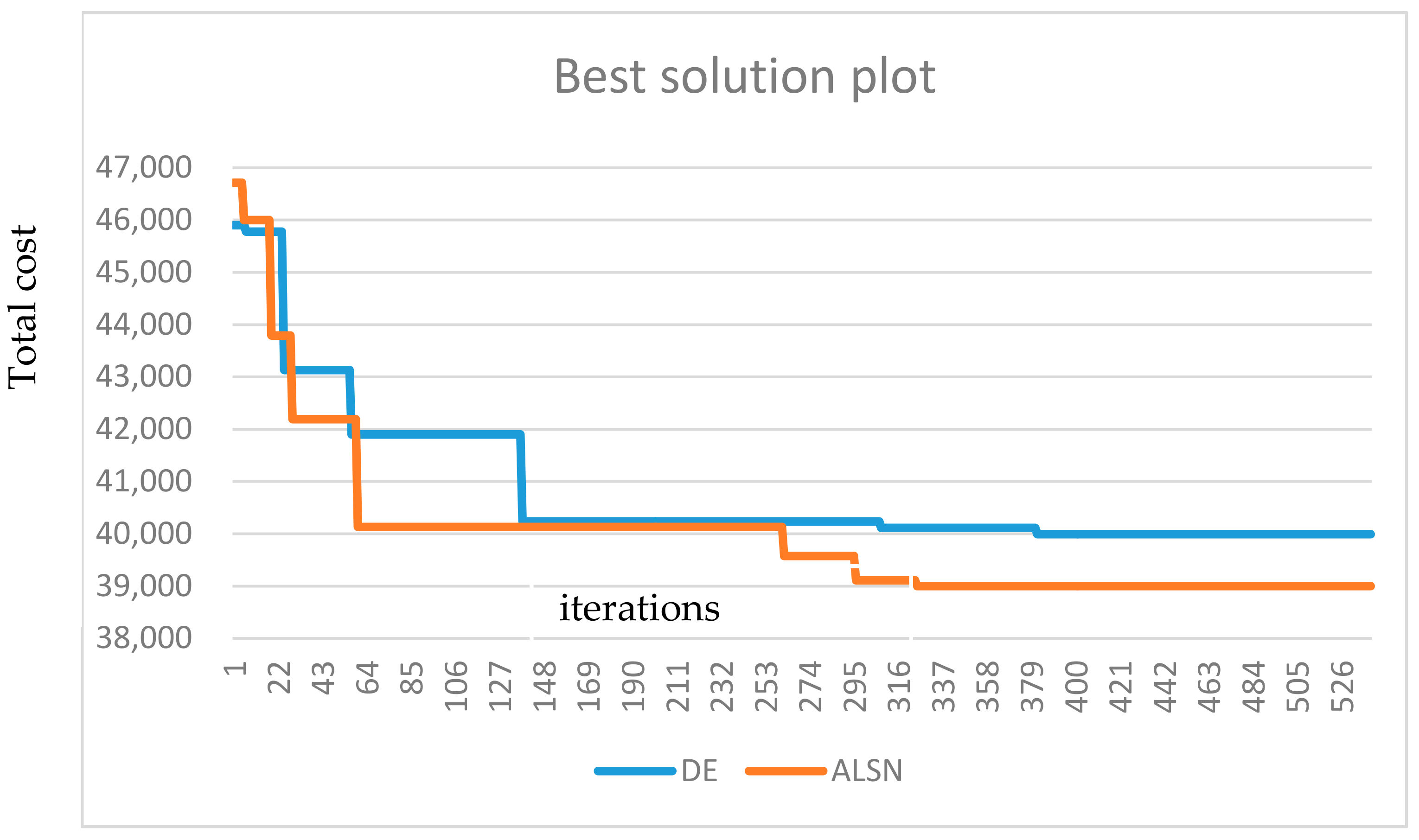
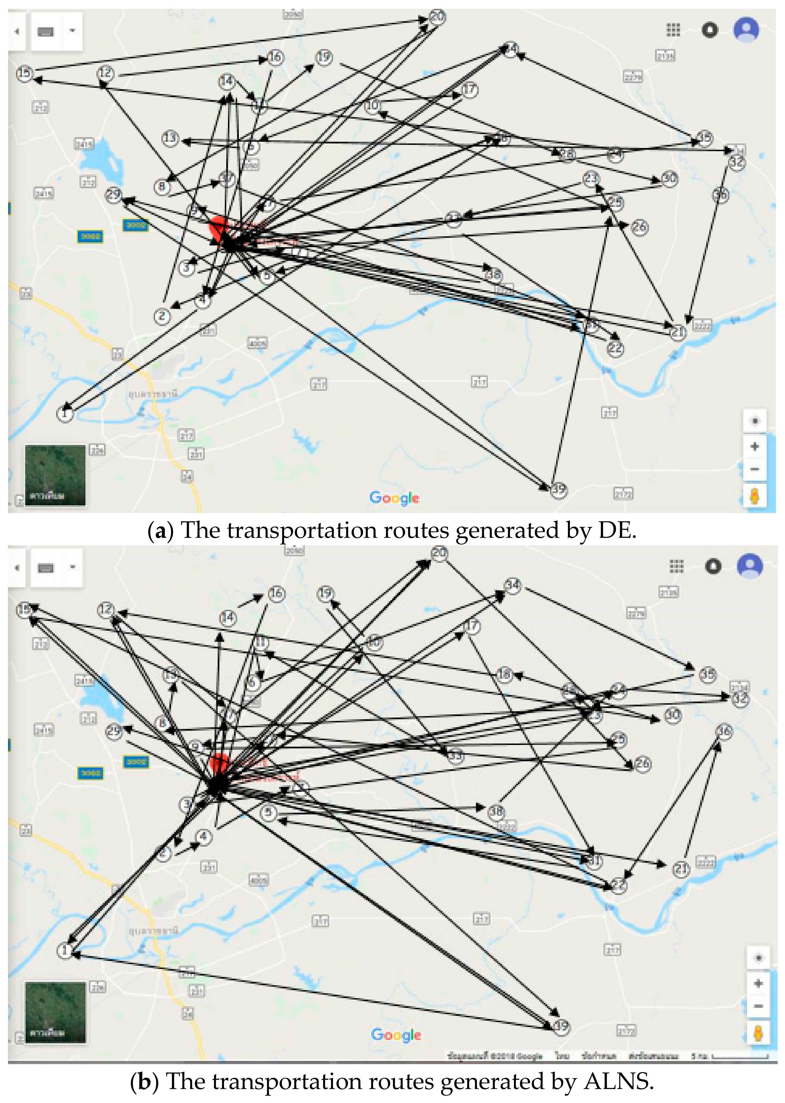
Figure 3 and Figure 4 show the nature of DE and ALNS in finding the solution for the case study. We can see that DE was better at searching for a good solution during the simulation run, while ALNS was more effective at finding a good solution. When the iteration was high, DE seemed to stick to the same local optimal, but ALNS made changes to the solution, which means that it had a better way than DE to escape from the local optimal solution.

5. Conclusions and Outlook

This paper presents a methodology to solve a special case of VRP, which makes simple VRP into a complex NP problem. We presented two metaheuristics, which were the differential evolution (DE) algorithm and the adaptive large neighborhood search (ALNS). DE was used to optimize the sequence of the bus stops that were assigned to buses that were randomly selected one at a time by roulette wheel selection. The attractiveness of the bus is the score of the bus, which is iteratively updated due to the quality of the solution contributed by the bus. In ALNS, six destroy methods and four repair methods were presented.

From the computational results, we can see that the proposed heuristics outperformed the best practices currently used in school systems. DE had an 8.89% lower cost than that of the current practice, while ALNS had 9.79% lower cost than that of the current practice. Calculations of the annual operational costs showed that DE could reduce the cost by 757,250 baht, while ALNS could reduce the cost by 906,750 baht from the current practice. When comparing the two proposed heuristics, ALNS had a lower cost than DE by 0.99% because ALNS had a mechanism that was better at escaping from the local optimal.

DE needs to add a local search or a restarting behavior so that it can find a better way to escape from the local optimal. ALNS may find a better solution if a variety of destroy and repair methods are applied.

The proposed heuristics are used as a tool in the development of effective and efficient user-friendly software. In addition to being effective and efficient, the software needs to be customized to satisfy customer needs. This is done by elucidating an effective algorithm to find solutions to satisfy customer needs. This research only shows the effectiveness of DE and ALNS in finding the most efficient solution. Future research should focus on satisfying customer needs. This may involve conducting primary research to identify what customers want and applying the findings to the algorithm.

Currently, the new emergent technology has been introduced to real-world situations regarding vehicle such as the driverless vehicle or the autonomous cars. It is composed of various up-to-date technologies such as radar, laser light, GPS, and computer vision. The advanced control system will be used to control the moving and routing of the car that is needed. The navigation system is necessary for this type of car to have the shortest, fastest, and cheapest route for the owner. Therefore, when the vehicle starts from the depot, without the driver, a good routing system will be calculated and used to control the car. When the car starts, it needs to move in such a way that the navigation system is shown, hence a fast and effective algorithm to show which route the vehicle have to travel is needed. Therefore, this research is applicable and suitable to install in the main brain of the driverless car so that it enhances the capability of the vehicle.

References

1. Dantzig, G.; Ramser, J. The truck dispatching problem. Manag. Sci. 1959, 6, 80–91. [Google Scholar] [CrossRef]
2. Lenstra, J.K.; Rinnooy Kan, A.H.G. Complexity of vehicle routing and scheduling problems. Networks 1981, 11, 221–227. [Google Scholar] [CrossRef] [Green Version]
3. Bettinelli, A.; Ceselli, A.; Righini, G. A branch-and-cut-and-price algorithm for the multi-depot heterogeneous vehicle routing problem with time windows. Transp. Res. 2011, 19, 723–740. [Google Scholar] [CrossRef]
4. Xu, Y.; Wang, L.; Yang, Y. A New Variable Neighborhood Search Algorithm for the Multi Depot Heterogeneous Vehicle Routing Problem with Time Windows. Electron. Notes Discret. Math. 2012, 39, 289–296. [Google Scholar] [CrossRef]
5. Dondo, R.G.; Cerda, J. A hybrid local improvement algorithm for large-scale multi-depot vehicle routing problems with time windows. Comput. Chem. Eng. 2009, 33, 513–530. [Google Scholar] [CrossRef]
6. Braekers, K.; Ramaekers, K.; Van Nieuwenhuyse, I. The vehicle routing problem: State of the art classification and review. Comput. Ind. Eng. 2015, 99, 300–313. [Google Scholar] [CrossRef]
7. Braekers, K.; Caris, A.; Janssens, G. A Deterministic Annealing Algorithm for a Bi-Objective Full Truckload Vehicle Routing Problem in Drayage Operations. Procedia Soc. Behav. Sci. 2011, 20, 344–353. [Google Scholar] [CrossRef]
8. Tsiropoulou, E.E.; Mitsis, G.; Papavassiliou, S. Interest-aware energy collection & resource management in machine to machine communications. Ad Hoc Netw. 2018, 68, 45–57. [Google Scholar]
9. Tsiropoulou, E.E.; Paruchuri, S.T.; Baras, J.S. Interest, energy and physical-aware coalition formation and resource allocation in smart IoT applications. In Proceedings of the 51st Annual Conference on Information Sciences and Systems (CISS), Baltimore, MD, USA, 22–24 March 2017; pp. 1–6. [Google Scholar]
10. Lin, C.R.; Gerla, M. Adaptive clustering for mobile wireless networks. IEEE J. Sel. Areas Commun. 1997, 15, 1265–1275. [Google Scholar] [CrossRef] [Green Version]
11. Wu, Y.; Khisti, A.; Xiao, C.; Caire, G.; Wong, K.K.; Gao, X. A Survey of Physical Layer Security Techniques for 5G Wireless Networks and Challenges Ahead. IEEE J. Sel. Areas Commun. 2018, 36, 679–695. [Google Scholar] [CrossRef] [Green Version]
12. Kim, G.; Ong, Y.S.; Heng, C.K.; Tan, P.S.; Zhang, N.A. City vehicle routing problem (city VRP): A review. IEEE Trans. Intel. Trans. Syst. 2015, 16, 1654–1666. [Google Scholar] [CrossRef]
13. Karakatič, S.; Podgorelec, V. A survey of genetic algorithms for solving multi depot vehicle routing problem. Appl. Soft Comput. 2015, 27, 519–532. [Google Scholar] [CrossRef]
14. Gupta, A.; Saini, S. On Solutions to Vehicle Routing Problems Using Swarm Optimization Techniques: A Review. In Advances in Computer and Computational Science; Springer: Singapore, 2017; pp. 345–354. [Google Scholar]
15. Hoff, A.; Løkketangen, A. A tabu search approach for milk collection in western Norway using trucks and trailers. In Proceedings of the Sixth Triennial Symposium on Transportation Analysis (TRISTAN VI), Bentota, Sri Lanka, 10–15 June 2007. [Google Scholar]
16. Tan, K.C.; Chew, Y.H.; Lee, L.H. A hybrid multi-objective evolutionary algorithm for solving truck and trailer vehicle routing problems. Eur. J. Oper. Res. 2006, 172, 855–885. [Google Scholar] [CrossRef]
17. Ombuki-Berman, B.; Hanshar, F.T. Using genetic algorithms for multi depot vehicle routing. In Bio-Inspired Algorithms for the Vehicle Routing Problem Studies in Computational Intelligence; Springer: Berlin/Heidelberg, Germany, 2009; Volume 161, pp. 77–99. [Google Scholar]
18. Weise, T.; Podlich, A.; Gorldt, C. Solving real-world vehicle routing problems with evolutionary algorithms. In Natural Intelligence for Scheduling, Planning and Packing Problems; Chiong, R., Dhakal, S., Eds.; Springer: Berlin/Heidelberg, Germany, 2010; pp. 29–53. [Google Scholar]
19. Pitakaso, R. Differential evolution algorithm for simple assembly line balancing type 1 (SALBP-1). J. Ind. Prod. Eng. 2015, 32, 104–114. [Google Scholar] [CrossRef]
20. Pitakaso, R.; Sethanan, K. Modified differential evolution algorithm for simple assembly line balancing with a limit on the number of machine types. Eng. Optim. 2015, 48, 253–271. [Google Scholar] [CrossRef]
21. López Cruz, I.L.; van Willigenburg, L.G.; van Straten, G. Optimal control of nitrate in lettuce by a hybrid approach: Differential evolution and adjustable control weight gradient algorithms. Comput. Electron. Agric. 2003, 40, 179–197. [Google Scholar] [CrossRef]
22. Liao, T.W.; Egbelu, P.J.; Chang, P.C. Two hybrid differential evolution algorithms for optimal inbound and outbound truck sequencing in cross docking operations. Appl. Soft Comput. 2012, 12, 3683–3697. [Google Scholar] [CrossRef]
23. Liao, T.W.; Egbelua, P.J.; Chang, P.C. Simultaneous dock assignment and sequencing of inbound trucks under a fixed outbound truck schedule in multi-door cross docking operations. Int. J. Prod. Econ. 2013, 141, 212–229. [Google Scholar] [CrossRef]
24. Hou, L.; Zhou, H.; Zhao, J. A novel discrete differential evolution algorithm for stochastic VRPSPD. J. Comput. Inf. Syst. 2010, 6, 2483–2491. [Google Scholar]
25. Dechampai, D.; Tanwanichkul, L.; Sethanan, K.; Pitakaso, R. A differential evolution algorithm for the capacitated VRP with flexibility of mixing pickup and delivery services and the maximum duration of a route in poultry industry. J. Intell. Manuf. 2015, 28, 1357–1376. [Google Scholar] [CrossRef]
26. Akkararungruangku, E.; Sasitorn, K. Modified Differential Evolution Algorithm Solving the Special Case of Location Routing Problem. Math. Comp. Appl. 2018, 23, 34. [Google Scholar] [CrossRef]
27. Teoh, B.E.; Ponnambalam, S.G.; Kanagara, G. Differential evolution algorithm with local search for capacitated vehicle routing problem. Int. J. Bio-Inspired Comput. 2013, 7, 321–342. [Google Scholar] [CrossRef]
28. Xu, H.; Wen, J. Differential Evolution Algorithm for the Optimization of the Vehicle Routing Problem in Logistics. In Proceedings of the 2012 Eighth International Conference on Computational Intelligence and Security, Guangzhou, China, 17–18 November 2012; pp. 48–51. [Google Scholar]
29. Mingyong, L.; Erbao, C. An improved differential evolution algorithm for vehicle routing problem with simultaneous pickups and deliveries and time windows. Eng. Appl. Art. Intel. 2010, 23, 188–195. [Google Scholar] [CrossRef]
30. Şahin, C.; Kuvvetli, Y. Differential evolution based meta-hueristic algorithm for dynamic continuous berth allocation problem. Appl. Math. Model. 2016, 40, 10679–10688. [Google Scholar] [CrossRef]
31. Sethanan, K.; Pitakaso, R. Differential evolution algorithms for scheduling raw milk transportation. Commun. Electron. Agric. 2016, 121, 245–259. [Google Scholar] [CrossRef]
32. Sethanan, K.; Pitakaso, R. Improved differential evolution algorithms for solving generalized assignment problem. Exp. Syst. Appl. 2016, 45, 450–459. [Google Scholar] [CrossRef]
33. Lampinen, J.; Zelinka, I. Mechanical engineering design optimization by differential evolution. In New Ideas in Optimization; Corne, D., Dorigo, M., Glover, F., Eds.; McGraw-Hill: London, UK, 1999; pp. 127–146. [Google Scholar]
34. Shaw, P. Using constraint programming and local search methods to solve vehicle routing problems. In Principles and Practice of Constraint Programming; Springer: Berlin/Heidelberg, Germany, 1998; pp. 417–431. [Google Scholar]
35. Aksen, D.; Kaya, O.; Salman, F.S.; Tuncel, O. An adaptive large neighborhood search algorithm for a selective and periodic inventory routing problem. Eur. J. Oper. Res. 2014, 239, 413–426. [Google Scholar] [CrossRef]
36. Azi, N.; Gendreau, M.; Potvin, J.-Y. An adaptive large neighborhood search for a vehicle routing problem with multiple routes. Comput. Oper. Res. 2014, 41, 167–173. [Google Scholar] [CrossRef]
37. Emec, U.; Catay, B.; Bozkaya, B. An Adaptive Large Neighborhood Search for an E-grocery Delivery Routing Problem. Comput. Oper. Res. 2016, 69, 109–125. [Google Scholar] [CrossRef]
38. Ribeiro Mattos, G.; Laporte, G. An adaptive large neighborhood search heuristic for the cumulative capacitated vehicle routing problem. Comput. Oper. Res. 2012, 39, 728–735. [Google Scholar] [CrossRef]
39. Hemmelmayr, C.V.; Cordeau, J.F.; Cranic, T. An adaptive large neighborhood search heuristic for Two-Echelon Vehicle Routing Problems arising in city logistics. Comput. Oper. Res. 2012, 39, 3215–3228. [Google Scholar] [CrossRef] [PubMed] [Green Version]
Figure 1. Problem definition explaining how the system works. Different sizes of vehicles are sent out to pick students up at bus stops of various sizes (different bus stops have a different number of students waiting).
Logistics 02 00015 g001
Figure 2. Example of cyclic move. The selected buses for the cyclic move are 3, 6, and 5. These three buses move cyclically. The detail of matching the destroy and repair methods is shown in Table 5.
Logistics 02 00015 g002
Figure 3. Behaviors of DE and ALNS during the simulation run.
Logistics 02 00015 g003
Figure 4. Results of the case study of DE (a) and ALNS (b). Transportation route of the case study generated by DE and ALNS.
Logistics 02 00015 g004