Scheduling Approach for the Simulation of a Sustainable Resource Supply Chain

Abstract

The general goal of waste management is to conserve resources and avoid negative environmental impacts. This paper deals with the optimization of logistics processes at an underground waste storage site by means of solving scheduling issues and reducing setup times, with the help of a simulation model. Specific to underground waste storage is the fact that it is often only a side business to actual mining. With limited capacity and resources, all legal requirements must be met, while the business should still be profitable. This paper discusses the improvement of a logistical system’s performance using machine scheduling approaches with the support of a plant simulation model. The process sequence is determined by means of a priority index. Genetic algorithms are then applied to improve the priority index to further increase performance. Results of the simulation model show that the performance of the logistics system can be increased by up to 400 percent, ensuring adequate system performance for current as well as future demand without changes to the system’s capacities and resources.

1. Introduction

At the end of each product life cycle there are basically five alternatives for dealing with waste: Avoidance, reuse, recycling, thermal or material utilization, and disposal. In current environmental and climate policy, a stronger focus is placed on life cycle management, the environmentally friendly use of raw materials, and the prevention and reuse of waste. However, there is still a large amount of resources that end up in thermal or material utilization, or in disposal. In addition to the widely known above-ground disposals, such as landfills, waste is also utilized and disposed in the cavities created by mining. This applies especially to environmentally-hazardous substances.

In general, if waste cannot be recycled, it must be permanently excluded from the recycling economy, with the aim of neither impairing human health nor endangering animals and plants. Furthermore, water bodies and soils should not be negatively affected. The term ‘waste disposal’ is taken to mean the dumping of waste, but in an environmentally friendly and thus demanding fashion. As with recycling, individual steps are planned before disposal: Providing, transporting, storing, handling, and depositing. According to the German Kreislaufwirtschaftsgesetz (KrWG) (which can be translated into Waste Management Act or Law on Closed Cycle Management) [1], it may be necessary to separate and treat waste for disposal. Different to recycling is the deposition (permanent storage) of the waste, which takes place exclusively in approved plants and facilities; these facilities are mostly landfills. Examples of other methods of disposal according to the KrWG are (cf. [2] (p. 50ff)):

-

Injection (e.g., injection of pump-able waste into boreholes, salt domes or natural cavities, etc.).

-

combustion on land or at sea.

-

surface application (e.g., disposal of liquid or muddy waste into pits, ponds or lagoons, etc.).

-

introduction to a body of water, the sea, or oceans.

The special challenge for underground disposal is that it is often only an ancillary business to mining, and therefore not the focus of business operations. This means that certain resources, e.g., the shaft, must be shared with the actual core business. Consequently, this leads to limited resources and capacities for the operations of underground waste disposal. Furthermore, rising raw material prices and possible future technological advances make it reasonable for certain resources to be stored separately from others and made easily accessible underground, in order to recover their residual value in the future. This in turn leads to increased handling times.

This paper is dedicated to the optimization of logistics processes using machine scheduling approaches in an underground storage site in Germany. In the example studied, waste disposal reaches its limits due to capacity bottlenecks and legal requirements. Despite existing market demand, the disposal of further quantities of waste is currently not possible without adjustments. The objective of the study is therefore to increase the number of waste disposals by means of an improved production plan, without additional structural or personnel investments.

To reach this goal, the process steps of the supply chain are transferred to classical questions of machine utilization or scheduling. In this instance of process planning, problems of the temporal allocation of activities to limited resources are considered, whereby different constraints are to be considered and specific goals are to be achieved [3]. In the context of production, sequence planning and scheduling require resource or machine reservation, which has established the concept of machine occupancy or utilization planning for scheduling [4]. In other words, scheduling “indicate[s] the detailed timetable of what work should be done, when it should be done and where should be done” [5].

The aim of this study is to determine whether logistical operators can be improved (e.g., by the reduction of setup times) by treating operators like machines in the science of factory planning and optimization. To this end, the individual logistics process steps are to be regarded as individual machines, and implemented in the simulation tool. One goal is the identification of bottlenecks in the process and the reduction of setup times. Classical approaches to solving problems of machine scheduling and sequence planning are procedures such as branch and bound, heuristic procedures, or the application of priority rules (e.g., random, first come first serve, shortest processing time, shortest weighted processing time or earliest due date) [6] (p. 374).

2. Problem Description

In the area under investigation, the logistical flow for waste storage must be optimized with the following boundary conditions:

-

The legal conditions allow for a maximum storage period in the above-ground buffer store of seven days (i.e., everything that is accepted in the incoming goods department must be moved underground in a timely manner).

-

The storage sequence must be optimized, as the different products must be stored at different locations. This results in time taken for setup, as the operators have to be transferred to different locations. Therefore, it makes sense to choose the storage sequence in such a way that as few setup processes (implementation of the underground storage technique) as possible are necessary.

-

The capacities for the transport and storage operators cannot be increased for cost reasons (e.g., number of empty containers, time window for underground transport via shaft, number of transports and loading and unloading of vehicles).

At present, the quantities of waste delivered cannot be disposed of on time. The aim is to pick the delivered quantities in such a way that as few underground unloading operations as possible are required. By simulating this scheduling approach it is to be verified whether it can dispose of the quantities on time. Furthermore, if the scheduling approach is positively evaluated, it should be checked whether the delivery quantities can be further increased.

2.1. Process Description

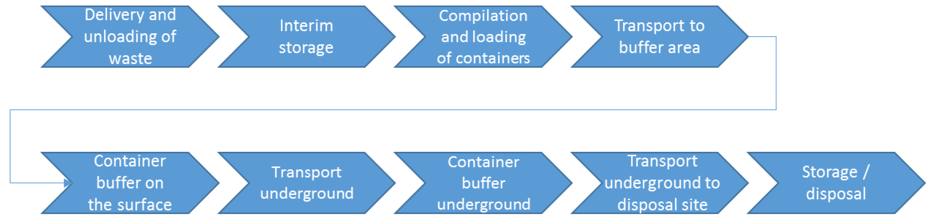
The analyzed process of underground waste storage and disposal can be separated into the following process steps:

• Delivery and unloading of the different types of waste (cf.

  Table 1. Overview of waste types.

  Substance Group	Description
  G1	Arsenic waste
  G2	Acid chemical residues
  G3	Alkaline chemical residues
  G4	Acid dry matter
  G5	Alkaline dry matter
  G6	Alkaline electroplating residues
  G7	Alkaline organic waste
  G8	Recyclable waste

  ), using different load carriers (Big-Bags, drums or steel containers).
• Interim storage in a warehouse (restrictions: Maximum storage period for waste types of seven days, capacity restriction of the storage quantity in the warehouse).
• Compilation and loading of empty containers in preparation for underground transport (restrictions: Only identical groups of substances may be loaded into one empty container, capacity restrictions on the mass and volume of empty containers, restrictions on the availability of empty containers).
• Transport of the containers to a buffer area.
• Buffering of the containers in front of the shaft lift (restriction: Maximum number in the buffer area).
• Transport of the containers underground by means of a shaft lift.
• Buffering of containers underground (restriction: Maximum number in the buffer area).
• Transport of the containers underground to the waste type-specific disposal location (restriction: Available transport operators).
• Unloading and securing the waste at the defined unloading locations (restriction: Available unloading operators).

The process can be summarized as shown in Figure 1.

As seen in the process description, the return transport of empty containers is not considered. It is assumed that a sufficient number of empty containers is always available. In the underground disposal site examined, waste in sixteen different substance groups can be disposed of. However, currently only eight groups are being processed, as shown in Table 1.

Different storage rooms are provided for each substance group. The waste delivered to the underground storage site is collected above ground, loaded into containers according to substance groups and then conveyed underground via an elevator shaft. There, they are picked up by transport vehicles and transported to the intended buffer areas. The final storage is then carried out with the aid of various load handling devices.

The seven groups of substances are delivered in three different containers: Big-Bags, bundles made of sheet steel drums, and sheet steel crates. Big-Bags and drum bundles are delivered on pallets for reasons of stability and handling. Generally, all waste must be packaged, although exceptions may apply to large appliances or containers upon agreement.

After delivery, the material groups are unloaded in the transfer hall and temporarily stored. A maximum interim storage of seven days is prescribed by law. Two forklifts are used to unload the trucks or load the roll-off containers, while a roll-off tipper is used to pick up and transport the containers between the transfer hall and a second shaft. The employees transport the groups of substances into designated transport containers. This container holds either four big-bags, three sheet steel containers or 12 bundles consisting of four sheet steel drums each, as long as the weight restriction is observed.

The next process step is to transport the containers underground through the shaft. The actual available time for material runs results from the shift length minus rope runs, changeover times between rope and material runs (10–15 min), as well as break times and times for testing the system. The net time available varies due to the number of rope rides, as well as maintenance and inspection measures. For example, a three-hour security check takes place weekly in the night shift on Sunday. In addition, there may be intermediate rope rides for visitors or the underground fire brigade.

Underground, a shaftman transports the roll-off containers from the large-area frame to the underground buffer area with another heavy-duty stacker. The roll-off containers are then transported to three different disposal locations by roll-off transport vehicles. There they are unloaded by means of (telescopic) forklifts. The three disposal sites are each intended for different groups of waste substances. While certain groups of substances must be disposed of separately (at different disposal locations), some groups of substances can be disposed of together at one location.

Every time the disposal location is changed, the telescopic forklift must be transferred to the new disposal location. Currently, the planning for this process is carried out manually without any system support. Because the transfer of the forklift is very time-consuming, setup times are comparably high. In summary, it can be stated as our objective in process optimization that the number of setup processes, and thus the setup times, must be minimized.

The described process has two characteristics, which are typical for flow shop scheduling problems. First, the maximum interim storage of seven days can be considered a product specific due date. Second, the substances are disposed of depending on their type of waste. If the disposal destination of substances differs from those of waste disposed of before, the company has to reconfigure the transportation system. In conclusion, the disposal process can be considered as a scheduling problem, whereby the transportation system acts as a single machine with waste specific setup groups, and the substances to dispose of represent the decision objects to schedule. In the following sections, we will shortly describe the theoretical principles of scheduling and present the mathematical optimization model for our problem.

3. Theoretical Principles of Scheduling

Scheduling, by definition, is the deployment of resources to complete a set of tasks during a determined time span. For instance, arrivals and departures of aircraft at an airport, courses and exam planning at an educational institution, dispatching jobs for production in a manufacturing environment and many decision-making processes in the service sectors are treated and studied under the scope of scheduling problems [7].

Scheduling problems are mathematically and formally described using three fields, α|β|γ, according to Graham et al. [8]. In the first field α, the machine environment and configuration are illustrated. The job characteristics are presented in the second field β. The objective functions are then described in the third field γ. Many authors tend to separate the job data and provide them separately to the problem formulation (cf. [8,9]).

Scheduling problems are classified based on different criteria, such as deterministic and stochastic scheduling [9], or flow and job shop scheduling [7]. Another criterion for classifying scheduling problems is the complexity degree of computing their solutions, since the adapted solution methodologies strongly rely on the complexity of an investigated problem. The optimal solution of a scheduling problem requires a complete search of the solution space. Searching the entire solution space of a problem implies enumerating all possible schedules to obtain the value of some objective function for each schedule. However, the number of possible schedules for even a small problem can easily grow exponentially. For instance, Gupta and Stafford [10] demonstrated the complexity of scheduling problems with a simple example, which involves scheduling five jobs to be processed on each of five machines in the same technological order. The problem is to be solved with respect to some objective function to reduce operational costs. They discussed the general case and demonstrated that the possible number of schedules was ${(5!)}^5$, even for such a small problem. They stressed how extensively expensive it is to fully explore all possible solutions.

One of the earliest works, and a comprehensive analysis of the complexity of scheduling problems, has been presented by Lenstra et al. [11]. The authors conducted a survey on the topic and classified standard scheduling problems into two groups. The first group contained most common scheduling problems that are NP-complete, while the other group was dedicated to problems solvable in polynomial time. They discussed the impact of some restrictions, constraints, and other parameters on the complexity of scheduling problems and their formulation. For instance, the sequence-dependent setup time constraint $s_{j,k}$ has a major impact on the complexity of scheduling problems [12]. Considering a problem with this constraint significantly increases its complexity, usually to the degree of NP-hardness, if the objective function is to minimize the makespan. For example, single machine scheduling problems are the easiest form of scheduling problems. Here, n number of jobs must be scheduled on one single machine. Yet, the $1\left|s_{j,k}\right|C_{max}$ problem, in which the objective function is to minimize the makespan under a sequence dependency constraint, is NP-Hard [13]. These complexity results can be derived by reduction to the well-known traveling salesman problem, which has been proven to be NP-Hard [14].

4. Formalization of the Scheduling Problem

Based on the process description of Section 2.1, we want to formulate the mathematical optimization problem. For this purpose, we adapt the conventional scheduling notation to our problem. Note that a job to be scheduled corresponds to a waste product to be disposed.

• Let $J\in \left\{J_1,\dots ,J_j\right\}:\mathsf{\forall }j\in \left\{1,\dots ,n\right\}$ denote a set of n jobs that must be scheduled.
• Let $p_{j,m}\in R_{+}$ denote the processing time to complete a job $J_j$ on machine m.
• Let $d_j\in N_{+}$ denote the due date of a job.
• Let $F=\left\{F_1,\dots ,F_f\right\}:\mathsf{\forall }f\in \left\{1,\dots ,3\right\}$ denote the set of the considered family in a dataset.
• Let $P=\left\{P_1,\dots ,P_p\right\}:\mathsf{\forall }p\in \left\{1,\dots ,8\right\}$ denote a set of the considered job types in a dataset.
• Let $P_p\subset F.$
• Let $\alpha =1$ be the number of machines considered.
• Let $\beta$ denote the required setup time to configure a machine m that was processing a job $J_j\in F_f$ to process a job $J_{j+1}\in {F^{\prime }}_f$ subject to Equation (1).

  $$\beta =45 \min$$

  (1)
• Let $T_j=max\left(c_j-d_j,0\right)$ be the delay of a job completed at the time $c_j$ late to its due date $d_j$.
• Let $U_j=\{\begin{array}{c}1if{c}_j>d_j\\ 0otherwise\end{array}$ be the penalty incurred due to a delayed job.
• Let ${\gamma }_1=T={{\displaystyle \sum }}_{j=1}^n{T}_j$ be the total delay of all jobs.
• Let ${\gamma }_2=U={{\displaystyle \sum }}_{j=1}^n{U}_j$ denote the total unit penalties incurred from the set of scheduled jobs.
• Based on the previous preliminaries and definitions, the investigated problem is $\alpha \left|\beta \right|{\displaystyle \sum }{T}_j,{\displaystyle \sum }{U}_j$.

Let $H$ denote the set of all possible schedules for a set of jobs $J_j$. Based on the mathematical formulation, it is desired to find a schedule $H\in H$, in which the set of jobs $J$ is scheduled on the machine. This schedule is then subject to the minimization of the total delay and the total penalties to produce all jobs as demonstrated in Equation (2).

$$\begin{array}{c}{\gamma }_1\left(H\right)={\displaystyle {\displaystyle \sum }_{j=1}^n}{T}_j,{\gamma }_2\left(H\right)={\displaystyle {\displaystyle \sum }_{j=1}^n}{U}_j\\ minZ\left(H\right)\iff min{\gamma }_1\left(H\right)\mathsf{\wedge }min{\gamma }_2\left(H\right):\mathsf{\forall }H\in H\end{array}$$

(2)

To solve the investigated problem, we adopted a weighted sum approach to formulate our objective function. From Equation (2), we can derive Equation (3).

$$arg\underset{H\in H}{min}Z\left(H\right)=W_1.{\gamma }_1+W_2.{\gamma }_2:\mathsf{\forall }\left(W_1+W_2=1\right),W\ge 0$$

(3)

5. Model Description

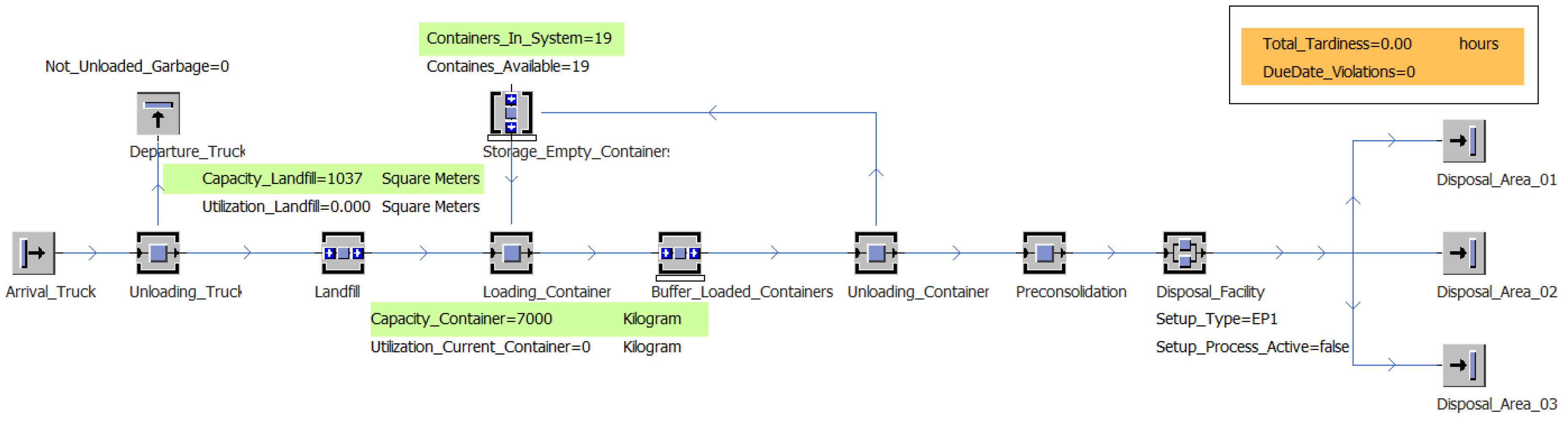
The processes of Section 2.1 were implemented in a simulation model, shown in Figure 2 below. The simulation model was implemented with Plant Simulation 14. Figure 2 only shows the implemented material flow. Control methods and auxiliary variables are hidden for clarity.

In the model, the source “Arrival_Truck” produces an entity representing a truck every 24 h. Before a truck leaves the source, a method defines what the truck has loaded. In the initial model, each truck loaded 25 waste units. The group of materials and the type of load carrier (big-bag, barrel or steel container) are randomly selected for each waste material via an uniform distribution. In the subsequent “Unloading_Truck” process, the waste is transferred from the truck to the landfill site. The transfer can only be carried out if the capacity of the landfill permits it. Waste units that cannot be taken up by the landfill leave the system again with the truck, and are noted in the meter variable “Not_Unloaded_Garbage”. During model initialization, the landfill is filled to approximately 80% of its capacity. The substance group and load carrier of the initial load are determined randomly, in accordance with the definition of the truck load. In the initial model, the waste units are stored according to the First-In-First Out (FIFO) principle. A priority index is introduced to prioritize the storage sequence. When the priority index is applied, the waste units are sorted according to descending indices. The sorting process always takes place as soon as:

• A new waste unit is moved on the storage area.
• A waste unit is moved from the storage area into a container.
• At the hour zero of each new day.

Since the number of containers prepared for the disposal plant is only known on a day-to-day basis, the retrieval of containers was modeled using a triangular distribution. Every 28 to 72 min, with an expected value of 48 min, the model takes an empty container from the “Storage_Empty_Containers” buffer and fills it with waste units from the same material group. The substance group is determined by the first waste object that is loaded into the container. If there are no empty containers, the process fails. Filled containers are temporarily stored in the “Buffer_Loaded_Containers” buffer until the waste disposal facility can receive and process them. The containers are retrieved according to the FIFO principle. In addition to the system’s capacity, the availability of the waste disposal system depends on its current setup. If the setup type of the system does not match the next container to be loaded, the system is blocked for 45 min and converted to the required type. For the disposal process, the waste is first removed from the container (model element “Unloading_Container”) and consolidated as a batch (model element “Preconsolidation”). The empty container is returned to the “Storage_Empty_Containers” buffer. The waste lot is then transferred to the disposal facility, where it remains for 45 min. Depending on the setup category, it then leaves the system via one of the three sinks, “Disposal_Area_01”, “Disposal_Area_02” or “Disposal_Area_03”.

5.1. Initial Situation

The first simulation run modeled the situation ‘as is’. The following process inputs were chosen:

• 100 days of simulation.
• 80% fill rate of the storage.
• 25 deliveries per day.
• 100 simulation runs.

This resulted in delays of 8195 h due to 176 delayed products. The system is therefore not suited to properly process the system inputs. 176 products would have been impossible to dispose of. This corresponds to the current situation and illustrates the need for optimization.

5.2. Implementation of a Priority Index (and Presentation of Results)

A priority index is introduced to optimize system behavior. It should change the sequence of processing in such a way that the number of setups is minimized, and the secondary condition of the maximum wait time of seven days is not exceeded. At this point, it was deliberately decided to use a priority index and not conventional optimization methods, such as metaheuristics.

The landfill currently has neither the necessary software nor appropriately trained personnel to have the daily disposal of waste calculated by a metaheuristic system. A priority index offers the advantage of providing a simple rule with the help of which the waste can be pre-sorted more efficiently. This enables a solution that is as easy to handle as possible to increase capacity through reduced setup times.

The developed priority index is based purely on logical considerations and is composed of the summands A, B, C and D. Each ID is calculated with its own index. As soon as a withdrawal from the warehouse takes place, this index is recalculated for each product. The priority index is structured as follows:

Four influencing variables (A, B, C, D) are to be included in the index, which is to be calculated according to product type and actual waste quantity and type. The four influencing variables are weighted and then summed. Waste IDs with a high priority index should then be given priority for waste storage.

Priority index = 0.1∗A + 0.2∗B + 0.2∗C + 0.5∗D

A: Probability of delivery on the next day (dependent on product type, based on the delivery probabilities over the last year):

For probabilities >30% set 2,

>20% set 1,

>10% set 0.5,

and <10% set 0.

B: Existing storage percentage (How big is the percentage of the total amount stored at this moment?):

For percentages >30% set 2, >20% set 1, >10% set 0.5, and <10% set 0.

• C: Storage duration of this ID
• 1 day set 0.1
• 2 days set 0.2
• 3 days set 0.5
• 4 days set 1
• 5 days set 2
• 6 days set 4
• 7 days set 10

• D: Does the setup currently correspond to this ID?
• True: set 1
• False: set 0

The introduction of the influence variables is initially based on an intuitive understanding of the problem. In the course of the analysis the weights of the influence variables are to be evaluated.

For simulation runs using the priority index to optimize storage, the same conditions were used as in the ‘as is’ simulation:

• 100 days of simulation
• 80% fill rate of the storage
• 25 deliveries per day
• 100 simulation runs

As a result, the sum of all delays could be reduced from 8195 h to 0 h and the number of delays were reduced from 176 to 0. This demonstrated that the use of a priority index could reduce setup times by a huge degree, and that the initial model can shoulder the system load by using different sequence planning.

5.3. Application of a Genetic Algorithm to Optimize the Priority Index

A further step examines whether the selection of the weightings of the priority index is optimal, or whether it can be improved. This optimization is to be carried out using a genetic algorithm. A genetic algorithm is chosen to optimize the weightings, because Plant Simulation already provides an optimization engine relying on a genetic algorithm. Thus, time could be saved by conceptualizing and implementing a custom optimization approach tailored to the discrete-event simulation model. Genetic algorithms are also very appropriate for our problem, as they search for solutions without requiring any information about the problem itself. This property is beneficial, since the available input data for the simulation model are highly aggregated which makes, for instance, the application of machine learning methods infeasible.

Genetic algorithms are metaheuristics belonging to the class of evolutionary algorithms. The term “Metaheuristic” comprises algorithms that guide the search for solutions to an optimization problem according to a specific pattern [15] (p. 270). The search methodology of evolutionary algorithms relies on the ideas of Charles Darwin’s theory of evolution, in particular on the principles of mutation and selection [16] (p. 110). There are several versions of genetic algorithms, but the basic process for determining solutions is always the same: In a first step, the genetic algorithm creates a set of initial solutions. This set of solutions is called the population. The creation of the initial population is random. However, despite the randomness, the algorithm tries to meet specific requirements for the initial population, for instance the achievement of a large-scale distribution of solutions across the complete search space. As soon as the initial population is determined, the evolutionary algorithm starts the iterative search for solutions. First, the algorithm defines a subset of the current best solutions. Second, the algorithm mutates the solutions within the subset to generate new solution candidates. Mutation means that single elements of a solution vector are manipulated in a specific manner. In addition, the algorithm can recombine two subset members to form a new solution. More precisely, the vectors of the parent solutions are mixed to create new child solutions. When the algorithm has generated a satisfying number of new solution candidates, it replaces the worst solution within the population by an equal number of subset members providing the best solutions. Afterwards, the algorithm deletes the subset and enters the next iteration.

The search space for each weight variable ranges from 0 to 1. The objective function corresponds to Formula (3). We assumed the values of 0.7 and 0.3 for the parameters $W_1$ and $W_2$, respectively.

The result of the optimization of the priority index provided the following summands:

• A: 0.1677
• B: 0.1078
• C: 0.4850
• D: 0.2375

The genetic algorithm test has shown that all four selected parameters must influence the priority index. The weightings are slightly different from the previously selected distribution. Since the delay time for the priority index without genetic optimization was already 0 h (thus, the first goal of the investigation was already fulfilled), an improvement is not visible. However, it can be assumed that further potential can be exploited in terms of delivery volumes, so that these can be increased as follows.

6. Results

The objective of this study was to increase the number of waste disposals through improved scheduling, without additional structural or personnel investment. The simulation results from the applied priority index and its optimization by a genetic algorithm suggest that this is possible, and that further potential exists. Up until now, daily delivery of 25 waste units has been permitted at the site examined. The following sensitivity analysis shows the number to which incoming waste deliveries can be increased without causing delays due to the non-storage of waste within the specified time (seven days). The first increase in incoming waste unit deliveries showed that, for the first time, deliveries could not be accepted at 94 deliveries per day, as the capacity limitation of the incoming warehouse would be broken.

A sensitivity analysis was performed to reveal the maximum load (how much more can the company put away or produce) using the following parameters:

• 100 days of simulation
• 80% initial filling of the warehouse
• 20 simulation runs

Table 2. Sensitivity analysis.

Waste Units (System Load) per Day	Sum of Delays in h	Number of Delayed Jobs
98	0.74	0.28
97	0.03	0.05
96	0.07	0.07
96	0.99	0.31
94	0.27	0.12
93	0	0
92	0	0
91	0	0
90	0	0

displays the results of the sensitivity analysis.

The results show that the maximum load of the company can be increased enormously. It is highly probable that the daily supply of waste units can be increased to up to 93 per day without the products to be used being delayed. Almost four times as much as in the current situation (without priority index) can be stored.

It can thus be shown that machine utilization approaches can be used for logistical optimization, to identify and implement improvements in the logistical process. In this example, almost 400% more products could be disposed of than in the current real environment. Thus, it can be shown that the cause for the current limited disposal quantities lies in production planning. The approaches chosen in this paper exceeded the objective by far, and prove that machine utilization approaches can be used.