Theoretical Investigation of Inorganic Particulate Matter: The Case of Water Adsorption on a NaCl Particle Model Studied Using Grand Canonical Monte Carlo Simulations

Abstract

Sodium chloride (NaCl) represents the principal component of atmospheric particulates of marine origin. To gain a molecular-level understanding of the adsorption process of water vapor on the NaCl surface, Monte Carlo simulations performed in the Grand Canonical ensemble were carried out, considering the water adsorption at different water pressures on a NaCl(001) surface. The calculated adsorption isotherm shows four different regions, whose coverages correspond to those of the low-, transition-, high-, and pre-solution-coverage regions experimentally observed. Detailed analysis reveals how the structure of the adsorbed water molecules (islands, layer, and multi-layer) changes depending on water pressure, and how their orientation with respect to the surface varies with the distance from the surface. This detailed information further supports the picture coming from previous experimental IR absorption spectroscopy studies.

1. Introduction

Atmospheric aerosols are colloidal systems with one phase, solid or liquid, dispersed in the gas phase and consist of either an inorganic or organic core (e.g., soluble salts, insoluble black carbon, soil, or soot), promoting the condensation of water as well as other organic and inorganic molecules and acting as a platform for chemical reactions [1]. Aerosols, of both natural and anthropogenic origins, play a pivotal role in affecting climate change [2,3,4,5,6] by altering various atmospheric processes, like Earth’s radiative balance [7,8], cloud formation [9,10,11], and air quality [12,13,14,15].

Water vapor, as one of the most abundant greenhouse gases in the Earth’s atmosphere, extensively interacts with atmospheric particulates (aerosols). The adsorption of water molecules onto particulate-aerosol surfaces depends on the relative humidity (RH) and significantly influences the physicochemical properties of the particles, such as their size, shape, and reactivity [16,17,18].

Among the wide variety of aerosol species, sodium chloride (NaCl) has gained significant attention due to its ubiquity in marine environments and its prevalence in various terrestrial sources, including sea spray, windblown dust, and volcanic emissions [19,20,21,22,23]. Understanding the behavior of NaCl aerosols, particularly their interaction with water molecules, is crucial for comprehending atmospheric processes on a global scale [22,24]. In particular, the adsorption of water on NaCl aerosols can catalyze chemical reactions in the atmosphere [25,26].

Water adsorption on pulverized NaCl crystals was experimentally studied by Barraclough and Hall [27], showing that at 25 °C, a water monolayer is present at a water vapor pressure of 12.8 × 10⁻³ atm. However, these results refer to a system rich in surface defects that can affect water adsorption, and they do not detail the structure of the adsorbed water molecules [28].

Foster and Ewing [29] conducted cutting-edge experiments employing Fourier Transform Infrared (FTIR) spectroscopy to study water adsorption on well-defined NaCl(001) at ambient temperature. They were able to quantitatively relate the integrated absorbances to coverage values, θ, which is the number of water molecules per NaCl ion pair at the (001) surface. To do so, they exploited the fact that the OH stretching vibrations are particularly sensitive probes of hydrogen bonding networks. In particular, they considered that the near-coincidence of the spectroscopic signature of thin-film water on NaCl(001), at 24 °C and above ~12 × 10⁻³ atm, to that of brine or liquid water suggests that the hydrogen bonding network in the adlayer is liquid-like. Therefore, they associated this adlayer with multilayer thin-film water. At lower pressures, e.g., below 9 × 10⁻³ atm, the band center is shifted to a value between the neat liquid value and that of nonhydrogen-bonded, e.g., gas phase, water OH vibrations; they associated this adlayer with thin-film water in submonolayer islands. As far as their adsorption isotherms are concerned, they exhibited distinctive features, manifesting in four distinct regions. In the low-coverage region (θ ≤ 0.5), a gradual rise in θ was observed as the pressure increased. This region was interpreted as small islands of water molecules adsorbed to the surface and bound together by hydrogen bonds. As θ approached approximately 0.5, a transition region (0.5 ≤ θ ≤ 2.5) emerged, marked by a rapid ascent in the isotherm that exhibited an inflection point at around θ = 1.5 and began to turn over around θ = 2.5. This region was interpreted as a co-existence of monolayer islands and multilayer thin-film structures. In the high-coverage region (2.5 ≤ θ ≤ 3.5), the coverage showed a gentle increase with pressure. This was interpreted as a full multilayer structure resembling that of liquid water. At θ = 3.5, another inflection point was observed. That was interpreted as the deliquescence threshold and the θ ≥ 3.5 region was called the pre-solution region. These results imply the existence of different water assemblages at low and high coverage.

Computational studies were also performed to investigate water adsorption on the NaCl(001) surface. Engkvist et al. [30] developed a new potential for the interaction between water and NaCl and used it in conjunction with the ASP-W4 model for bulk water to find out through energy minimization that at 0 K, monolayers of adsorbed water clusters exhibit many different structures with similar energies, highlighting the system’s complexity. However, at room temperature, NVT Metropolis–Monte Carlo calculations, i.e., simulations carried out by keeping constant the number of particles, the volume, and the temperature—revealed a drastically different behavior [31]. At low coverage, clustering into islands was observed, aligning with experimental findings. Remarkably, the clustering phenomenon exhibited insensitivity to the potential accuracy, as even the simple TIP4P water potential successfully predicted clustering. Conversely, at higher coverage, the ASP-W4 potential yielded a more organized adlayer compared to the TIP4P potential. Calculations employing the ASP-W4 potential exhibited good agreement with experimental data, bolstering the reliability of their findings.

Subsequently, other experimental and computational studies have succeeded in the study of water adsorption on the NaCl surface. Verdaguer et al. used scanning polarized force microscopy, combined with classical molecular dynamics (MD) simulations of a monolayer of water molecules on a NaCl slab at room temperature, to study the adsorption behavior of water molecules on cleaved NaCl(001) as a function of the relative humidity (RH) between <5% and 40% [32]. They observed that in dry conditions, the surface contact potential was more negative near atomic steps than over flat terraces; as the humidity was increased, the contact potential of the terraces became more negative and, at 40% RH, the surface-potential differences between steps and terraces vanished. These results were interpreted as the effect of a preferential anion solvation, initially localized near steps, that then involves the entire surface.

Yang et al. investigated the water adsorption on a NaCl (001) surface through MD simulation in the canonical ensemble at 80 K using density functional theory (DFT) [33], showing that beyond a 0.5 monolayer coverage, the water–water interaction becomes stronger than the water–surface interaction. Guo et al. used scanning tunneling microscopy (STM) to observe at 5 K the water monomer and tetramer on a NaCl(001) surface with a Au substrate [34]. Finally, in a recent work, Vlasov et al. used contact force spectroscopy to analyze the water adsorption on the (001) surface of NaCl under atmospheric conditions at 80% relative humidity [35]. The latter cited study as well as the preceding ones we have just mentioned presented breakthrough results in the context of the study of water adsorption on NaCl. However, none of the previous papers addressed the calculation of the adsorption isotherm and the comparison with the experimental counterpart. This task is relevant to check the reliability of the adopted interaction potentials, and to provide realistic models, at the atomic detail, of the adsorbed water molecules at different water pressures. Because our interest concerns the investigation of the adsorption and reactivity of volatile organic compounds on these wet surfaces, these models represent the starting point for the continuation of our future studies.

With NVT Metropolis–Monte Carlo, it is not possible to study the adsorption of water molecules on the NaCl surface as a function of water pressure (in other words, it is not possible to calculate isotherms for comparison with the experimental ones). Instead, one can only choose a fixed value of coverage and analyze the interaction of the adsorbate with the surface. To calculate isotherms, simulations in the Grand Canonical ensemble are needed. In this approach, the system is simulated in the Grand Canonical ensemble (μ,V,T), i.e., keeping constant the chemical potential, the volume, and the temperature. In each simulation, the chemical potential value is set, and the simulation starts inserting/deleting water molecules until equilibrium is reached. Thus, Grand Canonical Monte Carlo (GCMC) provides a way of sampling configurations with a weighting corresponding to the Grand Canonical ensemble, in which the number of molecules is allowed to fluctuate. At equilibrium, the number of molecules in the system oscillates around a constant value and the coverage can then be calculated and analyzed for each value of the chemical potential. In GCMC, it is possible to choose a selection criterion for the insertion/deletion of molecules that allows for the partial pressure to be used as a simulation parameter instead of the chemical potential [36,37]. With the aim of allowing a direct comparison with the experimental isotherms measured by Foster and Ewing [29], this approach was used in our simulations.

In this study, we performed for the first time a Grand Canonical Monte Carlo investigation of the adsorption of water molecules on the NaCl(001) surface. Our results show how water molecules assemble on the NaCl(001) surface at different pressures, in accordance with the hypotheses based on FTIR experiments.

2. Results and Discussion

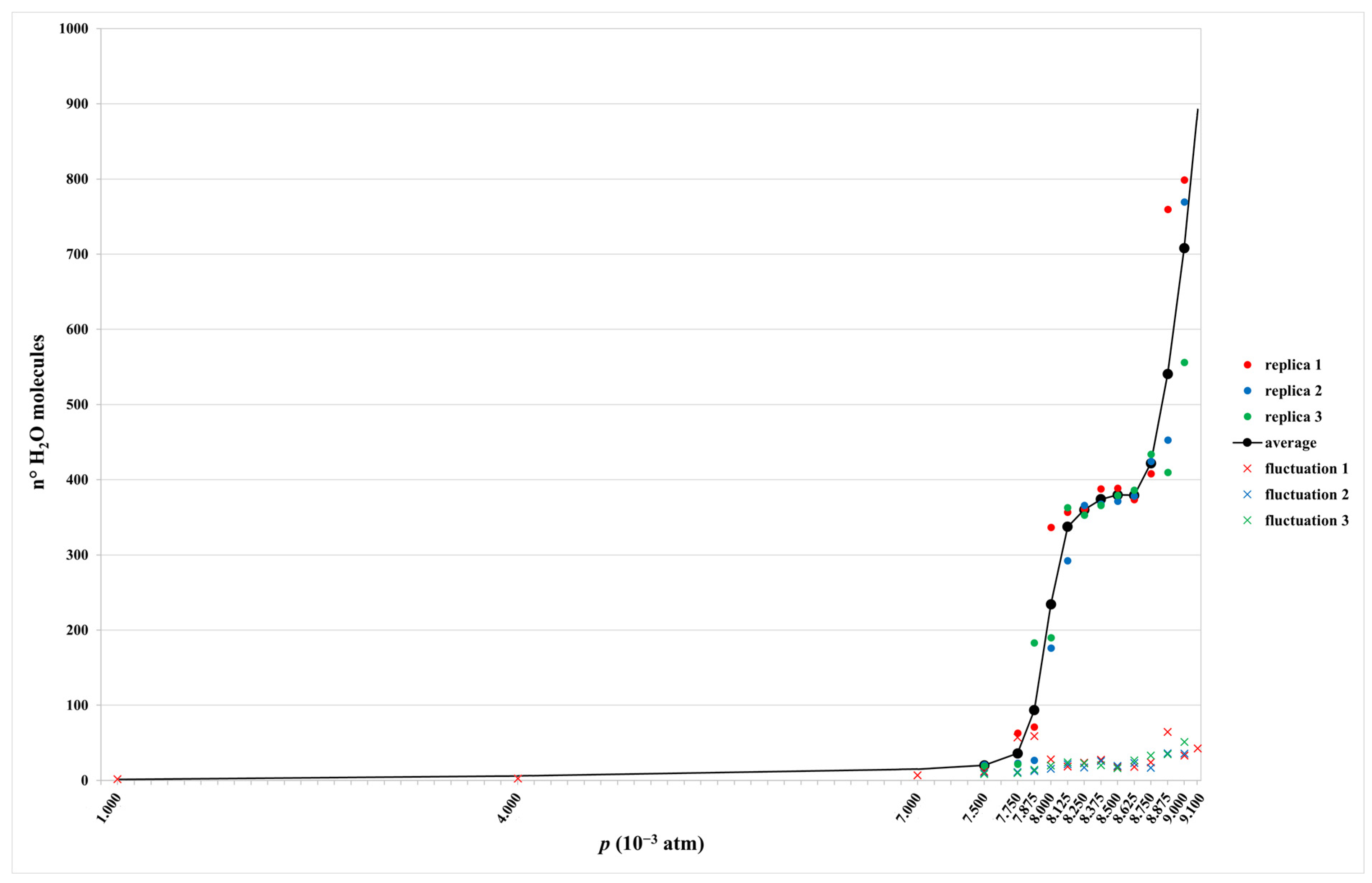
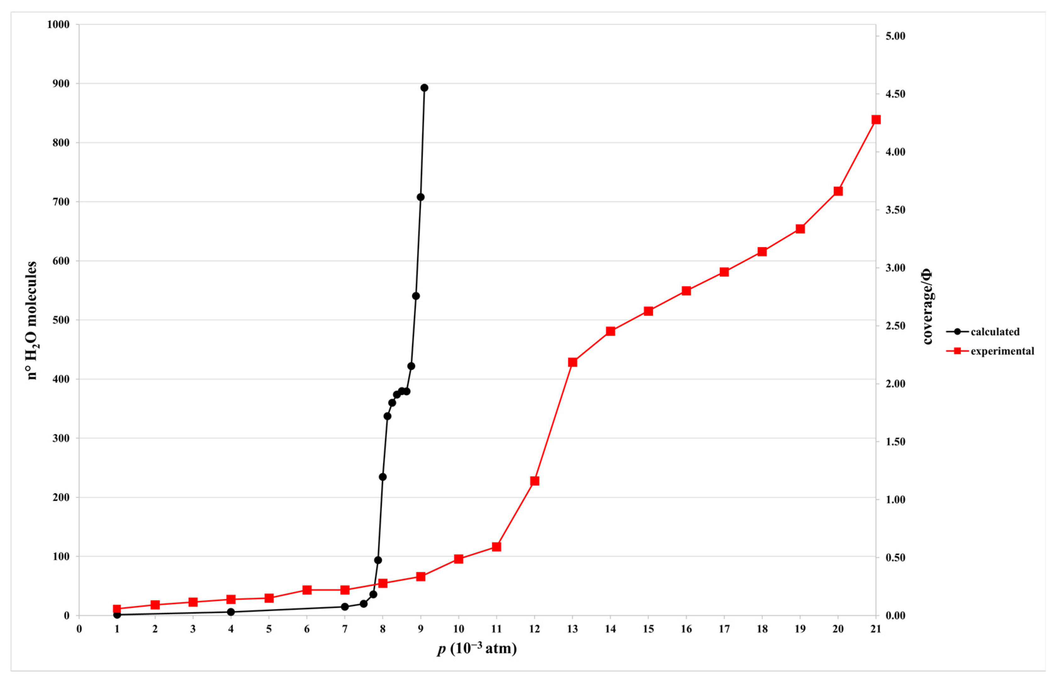
2.1. Isotherm

It is worth starting the analysis of our results by noting that we carried out simulations over a relatively wide pressure range, starting from the very low values considered in the reference experimental study [29] (i.e., from 1.000 × 10⁻³ atm). As highlighted in detail in the following, the water coverage of the NaCl surface up to 7.0 × 10⁻³ atm turned out to be very low, as expected. At the opposite extreme, the outcomes obtained at p > 9.000 × 10⁻³ atm correspond to the attainment of conditions such that the coverage (θ, see Section 3) is θ ≈ 5, which is a value experimentally found to lead to deliquescence; in this regard, it needs to be remarked that the study of the solubilization of NaCl at very high water coverage values is outside the scope of the present study.

The coverage, expressed both in terms of θ (see Section 3) and in terms of average values of the number of water molecules present in the system for each production simulation, is represented in Figure 1 and Figure 2. On the whole, a comparison between the calculated isotherm and the experimental one (see Figure 2) evidences that there are fundamental differences and a lack of consistency between them, despite some qualitative similarities, which are highlighted in the Supplementary Information (Figure S1). In the latter figure and in Figure 2, it can be noticed that in the simulations, the coverage increases up to deliquescence in a pressure range (from 7.5 × 10⁻³ atm to 9.1 × 10⁻³ atm) significantly narrower than in the experimental counterpart. A more detailed comparative analysis of the theoretical and experimental isotherms, including a focus on the abovementioned qualitative similarities, is proposed in the last part of the present paragraph, as attention now needs to be dedicated to the information that Figure 1 conveys on the fluctuations in the average number of water molecules occurring along the three replicates at the various pressure values. The greatest fluctuations in the average number of water molecules obtained for the three replicas are noted in correspondence with the simulations conducted at pressures of 8.000 × 10⁻³ atm and 8.875 × 10⁻³ atm, where the isotherm is characterized by a steep slope. Conversely, the two regions featuring small slopes (p < 7.875 × 10⁻³ atm and 8.125 × 10⁻³ atm < p < 8.875 × 10⁻³ atm) are generally characterized by small or very small fluctuations of H₂O molecules among the three replicas. As expected in the case of successful equilibration, each simulation in these regions shows that the number of water molecules starts fluctuating around an essentially constant value after an initial steep increase (see supporting information, Figure S2). As for the equilibration at points belonging to high-slope regions in the computed isotherm, the analysis needs to be informed by outcomes of a more detailed comparison between computed and experimental isotherms, which is presented in the following.

A notable point is that at pressures lower than 7 × 10⁻³ atm, a negligible water adsorption is observed in the simulations, while a smooth increase in the coverage is experimentally observed (see Figure 2). On the other hand, the coverage value associated with experimental deliquescence is observed around 20 × 10⁻³ atm, while the corresponding values obtained from simulations are around 9 × 10⁻³ atm. These findings suggest that the adopted force field potentials tend to underestimate the water-NaCl interactions and to overestimate the water–water interactions. However, analysis of the calculated isotherm reveals that it is possible to identify four different regions, corresponding to those ones highlighted in the experimental isotherm at similar coverage values (see Figure S1 and Figure 2). In fact, the first region is the one with low coverage and reaches a value of θ equal to 0.4; the second region is the transition region between θ = 0.4 and θ = 1.7; the third is the high-coverage region ranging from θ = 1.7 to θ = 2.5; and the final region is the pre-solution region for values of θ higher than 2.5. Transition and pre-solution regions feature steep slopes both in experiments and in theory; here, large fluctuations in the average number of water molecules among our replicas (see above and Figure 1) call for a detailed analysis of equilibration. For the transition region, during equilibration, the number of water molecules as a function of GCMC reaches values that oscillate around an almost constant value, as reported in SI and shown in Figure S3 for replicas at 8.000 × 10⁻³ atm. Most importantly, for the same replicas, histograms of the number of molecules present in the simulation box show a distribution that is essentially Gaussian, as expected in the case of successful equilibration (Figure 3).

A comparison between Figure 3 and Figure S3 evidences that, after an initial increase in the number of water molecules at some point preceding the last 300 million productive steps, replica 1 starts oscillating at a value of, ca., 340 water molecules, whereas in both replicas 2 and 3, oscillations persist at, ca., 180 water molecules; to better assess whether such a result is consistent with an overall equilibrium picture for our system, we decided to widely extend productive simulations by increasing more than tenfold the number of steps of the latter for replicas 1 and 2 (see SI, Figure S4). Notably, the resulting simulations encompassing more than 6 billion steps each demonstrate that the water molecules continue to oscillate around the values reported above for replicas 1 and 2. The presence of a lower number of water molecules in replicas 2 and 3 corresponds to the co-existence of a fully formed water layer on one face of the NaCl slab and of water molecule islands on the other face, which is consistent with the experimental picture for the transition region within the isotherm (vide infra, Section 2.2). As far as replica 1 is concerned, it shows a fully formed layer on both faces of the NaCl slab, which is also compatible with the local description of a fully water-covered region of a surface occurring in experiments. Although the outcomes of our efforts cannot guarantee that an overall equilibrated picture was actually reached for the transition region, the considerations reported above give us confidence about the fact that the simulations can provide useful chemical insights also in this case. This is corroborated by the observation that our theoretical representation of the transition region smoothly joins together the two well-equilibrated low-coverage and high-coverage isotherm portions, as expected (see Figure 1 and Figure S1).

As far as the pre-solution region is concerned, Figure 4 shows histograms of the number of molecules present in the simulation box for replicas at p = 8.875 × 10⁻³ atm; in this case, distributions significantly deviate from a Gaussian shape. Graphs of the number of water molecules as a function of GCMC steps (Figure S5) are in line with what is seen in Figure 1 for p = 8.875 × 10⁻³ atm, i.e., coverage values tend to differ among replicas. As the computational cost of GCMC simulations significantly increases along with the marked increase in the number of water molecules in the pre-solution region as compared to any other isotherm region analyzed here, equilibration appears to become more problematic as well. This is further illustrated by simulations carried out at p = 9.1 × 10⁻³ atm, in which the number of water molecules maintains the growing trend even when GCMC calculations are continued for 3.3 billion steps (see SI, Figure S6 for details), well beyond the 2.8 billion steps limit we imposed to most of the other simulations as a reasonable target for obtaining equilibrium conditions.

2.2. Identification of Water Aggregate Structures

The results presented in Section 2.1 indicate that simulations can provide reliable information on the organization of the water molecules on the NaCl surface during adsorption, even if the process takes place in a narrower range of pressures than the experimental one.

Now, in order to find groups of water molecules that could be interpreted as islands or layers on the NaCl surface, we analyzed the profiles of the density of the water molecules, defined by the position of the water oxygen atoms, as a function of the distance from the surface. The classification of water aggregates as islands was based on the data reported in the Supplementary Information (Table S1 and Figures S8–S10), and on the considerations reported there and in Methods. As far as fully covered surfaces are concerned, they were classified as monolayer-structured (about 150 water molecules), bilayer-structured (about 300 water molecules), or multilayer-structured (more than 450 water molecules).

Cluster analysis thus provides:

• The mean number (and standard error) of islands identified in each simulation, together with the mean number (and standard error) of water molecules contained in each island.
• The mean number (and standard error) of fully covered surfaces identified in each simulation, and the average number of water molecules on each surface. For example, a value equal to 1 will indicate that, on average, only one of the two NaCl surfaces is completely covered.
• The standard error of the mean ($S_{\underset{\_}{X}}$) is obtained as the ratio between the standard deviation associated with the set of values and the square root of the number of averaged values: $S_{\underset{\_}{X}}=\frac{s}{\sqrt{n}}$.

The results of the cluster analysis, which are shown in Tables S2–S4, mostly corroborate the interpretation of the experimental study by Foster and Ewing, as detailed in the following [29]. The results of simulations carried out under low coverage (θ ≤ 0.5), with p from 7.500 to 7.875 × 10⁻³ atm, confirm the constant presence of islands in the system—specifically, an average number that fluctuates between 1.5 and 2 islands per frame—that have small dimensions (6–10 water molecules per island). The observations are in agreement with the experimentally determined IR absorption frequency, which is related to the presence of two-dimensional aggregate formations with lateral hydrogen bonds that are midway between those of water in the gas and liquid phases. The simultaneous existence of layered structures and islands in some of the low-coverage simulations is a surprising outcome. In particular, in the third replica at 7.875 × 10⁻³ atm (Table S4), the formation of a permanent layer adsorbed on one of the two NaCl surfaces is observed (see Figure 5).

In the transition region (8.000–8.250 × 10⁻³ atm), data regarding p = 8.000 × 10⁻³ atm are analyzed only for the third replica, a choice that is supported by the fact that a great variability among the three replicas is observed at this pressure value; around such a value, where there is a large variability in the degree of coverage among replicas, it was decided to consider only the replica closest to the mean among the three replicas (see Figure 2). The results for the 8.000 × 10⁻³ atm water pressure are consistent with those obtained in the simulation run at 7.875 × 10⁻³ atm: on one of the two surfaces, a permanent layer has formed, while an island of varied size has formed on the other. A total covering of the two NaCl surfaces is present in all replicas at 8.125 and 8.250 × 10⁻³ atm (Tables S2–S4), with stratified structures made up of around 180 molecules on each surface, corresponding to a structure that is prone to a bilayer.

The results relating to simulations conducted in the high-coverage/pre-solution regions and, therefore, for water pressures between 8.375 and 9.000 × 10⁻³ atm, show that the two surfaces of NaCl are constantly completely covered. The size of the layers does not vary for pressure values between 8.375 and 8.625 × 10⁻³ atm; as shown in the calculated adsorption isotherm in Figure 2, this pressure range is characterized by a plateau region of the coverage. In particular, each layered structure is a bilayer, accommodating on average about 200 water molecules. From the pressure of 8.750 × 10⁻³ atm, the size of the layers starts to grow. In the first and second replicas (Tables S2 and S3) of the simulation conducted at 9.000 × 10⁻³ atm, i.e., the last pressure before deliquescence that underwent multiple-replica sampling, each of the two adsorbed layers has about 400 water molecules, a structure formed by four overlapping layers. In the third replica, a number of water molecules between approximately 250 and 300 per layer are reached.

In summary, the results confirm the structures of the adsorbed layer derived in the experimental study by Foster and Ewing [29]. However, contrary to what was reported in that study, the coexistence of islands and stratified structures does not only affect the transition region. The phenomenon is observable for water pressures close to the upper limit of the low-coverage region and in the first part of the pressure range characteristic of the transition region. Despite some differences, the trend in the number of islands and layers identified and in the size of the clusters, as a function of the water pressure, is quite consistent in the three replicas carried out for each simulation. The ability to obtain very similar results from the three replicas, starting from different initial conditions—i.e., from a different position of the single water molecule present in the first step of the equilibration phase—is an indication of good reproducibility of the simulations.

2.3. Orientation of Water Molecules as a Function of Distance from the NaCl Surface

The influence that the surface exerts on the water molecule orientation in the adsorbed layers was evaluated by considering the cosine of the angle, θ, between the opposite of the dipole moment vector of a water molecule and the normal vector to the surface (see Section 3).

For each replica, the following was obtained:

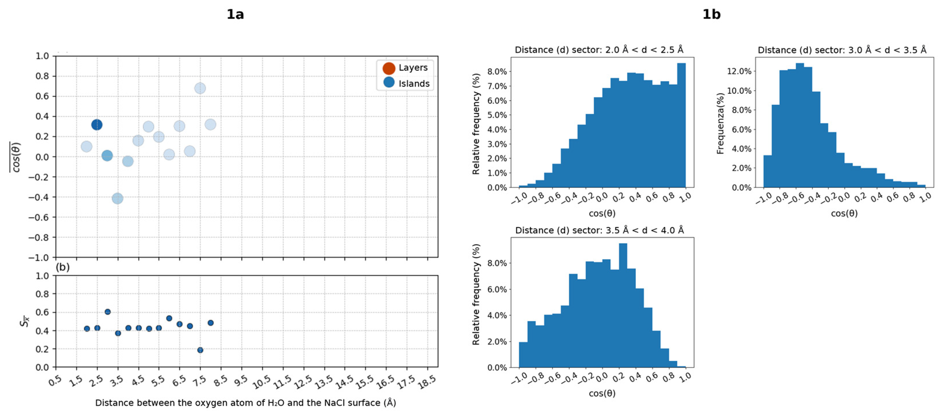
• A plot of the mean cos(θ) value of the water molecules as a function of the distance from the surface. In the plot, cos(θ) values of water molecules belonging to islands or layers are differently colored. The intensity of the color associated with each point of the graph is proportional to the number of averaged values. Each point of the graph, and thus each average value of cos(θ), has been obtained as the average of the orientations of all the water molecules that—during the analysis of the frames—have been classified as belonging to a certain “distance sector” from the NaCl surface. Each “distance sector” includes water molecules that have a distance value from the surface between two extremes separated by a step of 0.5 Å. Each average value will therefore be associated with a distance value from the surface, on the abscissa axis of the graph, which will indicate the upper limit of the “distance sector”. For example, a value of cos(θ), associated with a distance of 0.5 Å from the surface, is the average of the orientations of all water molecules characterized by a distance from the surface between 0 and 0.5 Å.
• For each “distance sector”, a histogram is generated, which represents the distribution of orientations in the entire simulation. The histogram is obtained by dividing the range of cos(θ) values, which go from −1 to +1, into intervals of 0.2 units. The intervals (on the x axis) define the basis of adjacent rectangles, whose height is the percentage frequency associated with the number of orientations identified in the specific interval. The frequencies shown are therefore relative frequencies, obtained from the ratio between the number of water molecules for which an orientation consistent with a certain interval has been determined, and the total number of water molecules belonging to the “distance sector”. The histogram is then normalized, and the sum of the heights of all the rectangles gives a percentage of 100%.

Representative graphs and histograms obtained for the two extreme coverage values (7.500 and 9.000 × 10⁻³ atm) are proposed in Figure 6.

Observing the graph relating to the simulation conducted in conditions of low coverage (Figure 6(1a)), it is possible to distinguish three values of cos(θ) relating to three “distance sectors” particularly relevant in the description of the islands that characterize the adsorbed water molecules. In the graph, there is a maximum corresponding to cos(θ) ≅ 0.4 ± 0.4 for 2.0 Å < d < 2.5 Å. The value and the standard error can be interpreted on the basis of the histogram (Figure 6(1b)) relating to the corresponding specific “distance sector”, in which a much higher relative frequency can be observed for values of cos(θ) > 0, and a maximum for cos(θ) ≅ +1. At a small distance from the surface, the water molecules in the islands will likely be positioned with one hydrogen atom pointing toward the surface (roughly for 0 < cos(θ) < 0.5, that is 60° < θ < 90) or with the oxygen atom on top of the Na⁺ cations (for 0.5 < cos(θ) < 1.0, that is 0° < θ < 60°)), with the hydrogen atoms directed away from the surface. Moving slightly away from the surface, there is a minimum for cos(θ) ≅ −0.4 ± 0.4 at 3.0 Å < d < 3.5 Å and the corresponding histogram shows a maximum relative frequency for −0.8 < cos(θ) < −0.4. The water molecules in this “distance sector” present the hydrogen atoms predominantly oriented toward the surface and will therefore be hydrogen bonded to the Cl⁻ anions. For an even greater distance, we have cos(θ) ≅ 0.0 ± 0.4, with loss of a preferential orientation. For greater distances, the number of water molecules identified is small, and the data are therefore of little relevance.

In the pre-solution simulations (Figure 6(2a)), cos(θ) presents maximum values for molecules very close to the surface; minimum values moving slightly away from it and oscillating, until stabilization; and values around zero for greater distance values. The behavior in the 2.0–3.5 Å region (Figure 6(2b)) resembles what has been observed in the low-coverage case (see above). A significant difference is observed instead for larger distances from the NaCl surface. In fact, the histogram in Figure 6(2b), correlated to a distance from the surface between 5.0 Å and 5.5 Å, shows a distribution that is comparable, although not perfectly, to a uniform distribution as expected for bulk water. The fact that the distribution is not perfectly homogeneous is probably due to the asymmetry of the system and therefore to a residual-orientating effect of the surface.

3. Methods

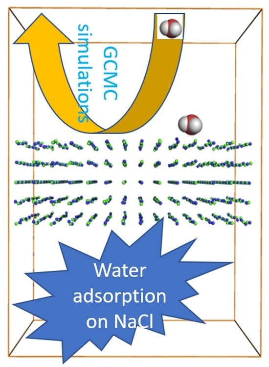
3.1. Grand Canonical Monte Carlo Simulations

The DL_MONTE program [37] was used to run GCMC simulations; this program builds on the highly successful DL_POLY molecular dynamics code and is designed to be complementary to it. In DL_MONTE, the GCMC simulations can be performed assuming two (equivalent) simulation control parameters: the chemical potential or the partial pressure of the gas [34,35]. In our calculations, we used the water pressure to allow a direct comparison with the experimental isotherms measured by Foster and Ewing [29].

The NaCl (001) surface was modeled as 5 layers of Na⁺ and Cl^- ions, each composed of 196 ions (98 Na⁺ and 98 Cl⁻ ions), placed at the center of a cell with sizes of 39.6 Å × 39.6 Å × 50.0 Å); thus, the system presents two surfaces exposed to the water vapor. It has to be noted that 50.0 Å is the maximum value that can be set within DL_MONTE for each of the three box dimensions. We checked the effects of reducing the size of the box along the z axis on the outcome of the productive simulation, taking replica 3 at p = 8.000 × 10⁻³ atm as a test case. In fact, as shown in SI, Figure S7, when the productive simulation is repeated after shrinking the box along the z axis to a value of 35.0 Å, the outcome of the 300-million-step GCMC run remains unaltered in essence. In this context, it needs to be underlined that such a shrinking of the box along the z axis leads to the overall volume not being occupied by water or NaCl, assuming a value comparable to that of the vacuum volume in the productive simulations carried out at the higher pressures within the theoretical isotherm shown in Figure 1. In the analysis of simulations, the coverage value (θ) is defined on the basis of the ratio between the number of water molecules and the number of Na⁺ cations present on the surface, assuming that θ = 1 corresponds to 196 H₂O in our model.

Although the mobility of all atoms of the NaCl slab should be required, we initially tried to reduce the computational effort by freezing first all the atoms of the slab and then allowing mobility of the different layers. These attempts (not reported) showed that to obtain reliable results, the mobility of the two outermost layers of each side of the slab was needed. Thus, during simulations, the ions of the two external layers of each side of the slab were allowed to move, while only those of the central layer were constrained to the crystallographic geometry.

Periodic boundary conditions were applied in all three spatial dimensions. Energies and coordinates were saved every 100 thousand steps.

A full non-bonded (only including point charges and van der Waals parameters) description of the NaCl surface was used according to the force field developed by Joung and Cheatham [38]; LJ parameters and point charges are reported in the Supplementary Information. The three-point model SPC/E was used for water molecules; note that the chosen force field for the description of NaCl was specifically developed to build better models of the monovalent ions, balancing crystal and solution properties in Ewald simulations including a well-known water model such as SPC/E [38]. Van der Waals and short-range Coulomb interactions were cut off at 1.2 nm, long-range Coulomb interactions were calculated using the Particle Mesh Ewald (PME) approach [39].

To compare our results with experimental data, the simulation temperature was set to 297.15 K. Water vapor pressure varied in the range of 1.0 to 9.1 × 10⁻³ atm. Three independent replicas were run for each pressure of water starting from a single initial water molecule (see Figure 7), apart from the cases of simulations with very low coverages (p < 7.5 × 10⁻³ atm) or with no apparent tendency toward equilibration (p > 9.0 × 10⁻³ atm), for which GCMC runs were singly performed. Each simulation consisted of an equilibration run and a subsequent productive run; equilibrations were carried out for 2.5 billion steps, apart from the cases of simulations with very low coverages (p < 7.5 × 10⁻³ atm); in the latter cases, 200 million steps equilibrations were performed. As far as the productive portions of simulations were concerned, they were 300 million for all simulations at the various pressure values, unless otherwise stated. Once equilibration was achieved in each simulation, the arrangement of the water molecules with respect to the surface was analyzed to identify the formation of sub-monolayers (at lower pressure values) and/or adsorbed layers of water. Additionally, the density of water molecules at increasing distances from the surface was evaluated to characterize the water layers present in the system. These analyses were conducted on the output of the three independent replicas performed for each pressure value considered.

3.2. Cluster Analysis

In order to find groups of water molecules that could be interpreted as islands or layers on the NaCl surface, a cluster analysis was performed by means of the DBSCAN (Density-Based Spatial Clustering of Applications with Noise) algorithm [40] on the GCMC sampling. DBSCAN classifies a point P in a dataset as the core point of a cluster if there are at least a threshold number (minPts) of other points within a minimum distance (ε) from P. In our case, the points were the oxygen (O) atoms of water molecules, ε was set to 4 Å, and minPts was set to 3.

Starting from a randomly selected unvisited oxygen atom, DBSCAN was used to perform a density-based region query to retrieve all neighboring O atoms within ε. If the number of retrieved O atoms was equal to or greater than the minPts threshold, a dense region was identified. Subsequently, we expanded the cluster by recursively assigning all directly reachable O atoms in the neighborhood to the same cluster as the current atom. This iterative process involved adding new O atoms to the cluster and exploring their own neighborhoods. We repeated this process for each unvisited O atom in the ensemble until all atoms were processed. The resulting clusters represented groups of water molecules with spatial proximity, while the unassigned oxygen atoms denoted isolated water molecules or noise. Clusters with less than 70 water molecules were classified as islands and clusters with more than 70 water molecules were classified as layers.

3.3. Analysis of the Influence of NaCl Surface on Orientation of Adsorbed H₂O Molecules

In order to investigate how the surface influences the water molecule orientation in the adsorbed layers, the cosine dependence of the θ angle was studied as a function of the distance from the surface. The θ angle is defined as the angle between the opposite of the dipole moment vector of a water molecule and the normal vector to the surface: cos θ = +1 (θ = 0°) denotes a water molecule arranged with the opposite dipole moment perpendicular to the surface, with the oxygen atom facing the surface and the hydrogen atoms moving away from it; cos θ = 0 (θ = 90°) denotes a water molecule arranged with the opposite dipole moment oriented parallel to the surface; cos θ = −1 (θ = 180°) denotes a water molecule arranged with the opposite dipole moment perpendicular to the surface, with the hydrogen atoms facing the surface and the oxygen atom moving away from it.

4. Conclusions

In this study, the Monte Carlo method applied in the Grand Canonical ensemble (GCMC) was employed with the aim of studying the interaction of water with the surface (001) of a crystal of solid sodium chloride. The latter constitutes one of the main components of atmospheric particulate matter of marine origin.

For each pressure value in the 7.5–9.0 × 10⁻³ atm range, three GCMC replicas were performed. In this range, simulations aiming at system equilibration were conducted for a total of 2 billion and 500 million steps followed by 300 million steps of production simulations on which the analyses were carried out.

A comparison of the calculated and experimental isotherms shows that in the former, the coverage increases up to deliquescence in a narrow pressure range. However, it is possible to identify four different regions, whose coverages correspond to those of the low-, transition-, high-, and pre-solution-coverage regions observed experimentally. This indicates that simulations can provide reliable information on the organization of the water molecules on this surface during the adsorption process.

The cluster analysis of the water molecules shows that in the low-coverage region (θ ≤ 0.4), they form small islands on the NaCl surface. Water molecules close to the surface (within 2.5 Å) preferentially adopt an orientation with the oxygen atoms directed toward the surface, while in the 3.0–3.5 Å range, the preferred orientation is such that the hydrogen atoms are oriented toward the surface.

In the transition-coverage region (0.4 ≤ θ ≤ 1.7), a co-presence of islands and mono/bi-layers is observed, while only multi-layer structures are observed in the high-coverage (1.7 ≤ θ ≤ 2.5) and pre-solution (θ ≥ 2.5) regions. When a multi-layer is reached, the orientation of the water molecules close to the surface resembles what has been observed in the low-coverage case (see above), while for larger distances from the NaCl surface, a distribution comparable to that expected for bulk water is observed.

In conclusion, the possibility of individually analyzing all the configurations generated by the simulations has made it possible to obtain a detailed view, at a microscopic level, of the adsorption process of water on model surfaces of atmospheric NaCl particulates, thus not only supporting the picture coming from the experimental IR absorption spectroscopy studies but also providing realistic models in atomistic detail for further investigation of the adsorption and reactivity of volatile organic compounds on these wet surfaces. As far as the water-NaCl interplay is specifically concerned, the results presented here are expected to be functional for future theoretical studies of the free energy profile of water interaction with NaCl surfaces at various coverage values by means of MD- or MC-based simulations.

References

1. Putaud, J.-P.; Van Dingenen, R.; Alastuey, A.; Bauer, H.; Birmili, W.; Cyrys, J.; Flentje, H.; Fuzzi, S.; Gehrig, R.; Hansson, H.C.; et al. A European Aerosol Phenomenology–3: Physical and Chemical Characteristics of Particulate Matter from 60 Rural, Urban, and Kerbside Sites across Europe. Atmos. Environ. 2010, 44, 1308–1320. [Google Scholar] [CrossRef]
2. Zhang, B. The Effect of Aerosols to Climate Change and Society. J. Geosci. Environ. Prot. 2020, 8, 55–78. [Google Scholar] [CrossRef]
3. Andreae, M.O.; Jones, C.D.; Cox, P.M. Strong Present-Day Aerosol Cooling Implies a Hot Future. Nature 2005, 435, 1187–1190. [Google Scholar] [CrossRef] [PubMed]
4. Watson-Parris, D.; Smith, C.J. Large Uncertainty in Future Warming Due to Aerosol Forcing. Nat. Clim. Chang. 2022, 12, 1111–1113. [Google Scholar] [CrossRef]
5. Ramanathan, V.C.; Crutzen, P.J.; Kiehl, J.T.; Rosenfeld, D. Aerosols, Climate, and the Hydrological Cycle. Science 2001, 294, 2119–2124. [Google Scholar] [CrossRef] [PubMed]
6. Boucher, O. Atmospheric Aerosols: Properties and Climate Impacts; Springer: Berlin/Heidelberg, Germany, 2015; ISBN 9789401796491. [Google Scholar]
7. Charlson, R.J.; Langner, J.; Rodhe, H.; Leovy, C.B.; Warren, S.G. Perturbation of the Northern Hemisphere Radiative Balance by Backscattering from Anthropogenic Sulfate Aerosols. Tellus A Dyn. 1991, 43, 152. [Google Scholar]
8. Andrews, E.; Ogren, J.A.; Bonasoni, P.; Marinoni, A.; Cuevas, E.; Rodríguez, S.; Sun, J.Y.; Jaffe, D.A.; Fischer, E.V.; Baltensperger, U.; et al. Climatology of Aerosol Radiative Properties in the Free Troposphere. Atmos. Res. 2011, 102, 365–393. [Google Scholar] [CrossRef]
9. Stevens, B.; Feingold, G. Untangling Aerosol Effects on Clouds and Precipitation in a Buffered System. Nature 2009, 461, 607–613. [Google Scholar] [CrossRef]
10. Carslaw, K.S.; Lee, L.A.; Reddington, C.L.; Pringle, K.J.; Rap, A.; Forster, P.M.; Mann, G.W.; Spracklen, D.V.; Woodhouse, M.T.; Regayre, L.A.; et al. Large Contribution of Natural Aerosols to Uncertainty in Indirect Forcing. Nature 2013, 503, 67–71. [Google Scholar] [CrossRef]
11. Lohmann, U.; Feichter, J. Global Indirect Aerosol Effects: A Review. Atmos. Chem. Phys. 2005, 5, 715–737. [Google Scholar] [CrossRef]
12. Davidson, C.I.; Phalen, R.F.; Solomon, P.A. Airborne Particulate Matter and Human Health: A Review. Aerosol Sci. Technol. 2007, 39, 737–749. [Google Scholar] [CrossRef]
13. Lighty, J.S.; Veranth, J.M.; Sarofim, A.F. Combustion Aerosols: Factors Governing Their Size and Composition and Implications to Human Health. J. Air Waste Manag. Assoc. 2011, 50, 1565–1618. [Google Scholar] [CrossRef] [PubMed]
14. Arden Pope, C., III; Burnett, R.T.; Thurston, G.D.; Thun, M.J.; Calle, E.E.; Krewski, D.; Godleski, J.J. Cardiovascular Mortality and Long-Term Exposure to Particulate Air Pollution. Circulation 2004, 109, 71–77. [Google Scholar] [CrossRef] [PubMed]
15. Bernstein, J.A.; Neil Alexis, C.B.; Leonard Bernstein, I.; Nel, A.; Peden, D.; Diaz-Sanchez, D.; Tarlo, S.M.; Brock Williams, P.; Bernstein, J.A. Health Effects of Air Pollution. J. Allergy Clin. Immunol. 2004, 114, 1116–1123. [Google Scholar] [CrossRef]
16. Tang, M.; Chan, C.K.; Li, Y.J.; Su, H.; Ma, Q.; Wu, Z.; Zhang, G.; Wang, Z.; Ge, M.; Hu, M.; et al. A Review of Experimental Techniques for Aerosol Hygroscopicity Studies. Atmos. Chem. Phys. 2019, 19, 12631–12686. [Google Scholar] [CrossRef]
17. Tang, M.; Cziczo, D.J.; Grassian, V.H. Interactions of Water with Mineral Dust Aerosol: Water Adsorption, Hygroscopicity, Cloud Condensation, and Ice Nucleation. Chem. Rev. 2016, 116, 4205–4259. [Google Scholar] [CrossRef]
18. Valsaraj, K.T. A Review of the Aqueous Aerosol Surface Chemistry in the Atmospheric Context. Open J. Phys. Chem. 2012, 2, 58–66. [Google Scholar] [CrossRef]
19. Sandu, I.; Chirazi, M.; Canache, M.; Sandu, I.G.; Alexianu, M.T.; Sandu, A.V.; Vasilache, V. Research on Nacl Saline Aerosols I. Natural and Artificial Sources and Their Implications. J. Environ. Eng. Landsc. Manag. 2010, 9, 881–888. [Google Scholar] [CrossRef]
20. Sandu, I.; Chirazi, M.; Sandu, I.G. Research on Nacl Saline Aerosols II. New Artificial Halochamber Characteristics. Environmentalist 2010, 9, 1105–1113. [Google Scholar] [CrossRef]
21. Wang, H.; Wang, X.; Yang, X.; Li, W.; Xue, L.; Wang, T.; Chen, J.; Wang, W. Others Mixed Chloride Aerosols and Their Atmospheric Implications: A Review. Aerosol Air Qual. Res. 2017, 17, 878–887. [Google Scholar] [CrossRef]
22. Finlayson-Pitts, B.J. The Tropospheric Chemistry of Sea Salt: A Molecular-Level View of the Chemistry of NaCl and NaBr. Chem. Rev. 2003, 103, 4801–4822. [Google Scholar] [CrossRef] [PubMed]
23. Chi, J.W.; Li, W.J.; Zhang, D.Z.; Zhang, J.C.; Lin, Y.T.; Shen, X.J.; Sun, J.Y.; Chen, J.M.; Zhang, X.Y.; Zhang, Y.M.; et al. Sea Salt Aerosols as a Reactive Surface for Inorganic and Organic Acidic Gases in the Arctic Troposphere. Atmos. Chem. Phys. 2015, 15, 11341–11353. [Google Scholar] [CrossRef]
24. David, D.; Weis, G.E.E. Water Content and Morphology of Sodium Chloride Aerosol Particles. J. Geophys. Res. 1999, 104, 21275–21285. [Google Scholar]
25. Davies, J.A.; Cox, R.A. Kinetics of the Heterogeneous Reaction of HNO3 with NaCl: Effect of Water Vapor. J. Phys. Chem. A 1998, 102, 7631–7642. [Google Scholar] [CrossRef]
26. Allen, H.C.; Laux, J.M.; Vogt, R.; Finlayson-Pitts, B.J.; Hemminger, J.C. Water-Induced Reorganization of Ultrathin Nitrate Films on NaCl: Implications for the Tropospheric Chemistry of Sea Salt Particles. J. Phys. Chem. 1996, 100, 6371–6375. [Google Scholar] [CrossRef]
27. Barraclough, P.B.; Hall, P.G. The Adsorption of Water Vapour by Lithium Fluoride, Sodium Fluoride and Sodium Chloride. Surf. Sci. 1974, 46, 393–417. [Google Scholar] [CrossRef]
28. Peters, S.J.; Ewing, G.E. Thin Film Water on NaCl(100) under Ambient Conditions: An Infrared Study. Langmuir 1997, 13, 6345–6348. [Google Scholar] [CrossRef]
29. Foster, M.C.; Ewing, G.E. Adsorption of Water on the NaCl(001) Surface. II. An Infrared Study at Ambient Temperatures. J. Chem. Phys. 2000, 112, 6817–6826. [Google Scholar] [CrossRef]
30. Engkvist, O.; Stone, A.J. Adsorption of Water on NaCl(001). I. Intermolecular Potentials and Low Temperature Structures. J. Chem. Phys. 1999, 110, 12089–12096. [Google Scholar] [CrossRef]
31. Engkvist, O.; Stone, A.J. Adsorption of Water on the NaCl(001) Surface. III. Monte Carlo Simulations at Ambient Temperatures. J. Chem. Phys. 2000, 112, 6827–6833. [Google Scholar] [CrossRef]
32. Verdaguer, A.; Sacha, G.M.; Luna, M.; Ogletree, D.F.; Salmeron, M. Initial Stages of Water Adsorption on NaCl (100) Studied by Scanning Polarization Force Microscopy. J. Chem. Phys. 2005, 123, 124703. [Google Scholar] [CrossRef] [PubMed]
33. Yang, Y.; Meng, S.; Wang, E.G. Water Adsorption on a NaCl (001) Surface: A Density Functional Theory Study. Phys. Rev. B Condens. Matter Mater. Phys. 2006, 74, 245409. [Google Scholar] [CrossRef]
34. Guo, J.; Meng, X.; Chen, J.; Peng, J.; Sheng, J.; Li, X.-Z.; Xu, L.; Shi, J.-R.; Wang, E.; Jiang, Y. Real-Space Imaging of Interfacial Water with Submolecular Resolution. Nat. Mater. 2014, 13, 184–189. [Google Scholar] [CrossRef] [PubMed]
35. Vlasov, V.P.; Muslimov, A.E.; Kanevsky, V.M. Water Adsorption on the (001) Surface of NaCl. J. Surf. Investig. X-ray Synchrotron Neutron Tech. 2020, 14, 1040–1043. [Google Scholar] [CrossRef]
36. Frenkel, D.; Smit, B. Understanding Molecular Simulation; Elsevier Science & Technology: Amsterdam, The Netherlands, 2002; ISBN 9786611019747. [Google Scholar]
37. Purton, J.A.; Crabtree, J.C.; Parker, S.C. DL_MONTE: A General Purpose Program for Parallel Monte Carlo Simulation. Mol. Simul. 2013, 39, 1240–1252. [Google Scholar] [CrossRef]
38. Joung, I.S.; Cheatham, T.E., 3rd. Molecular Dynamics Simulations of the Dynamic and Energetic Properties of Alkali and Halide Ions Using Water-Model-Specific Ion Parameters. J. Phys. Chem. B 2009, 113, 13279–13290. [Google Scholar] [CrossRef]
39. Essmann, U.; Perera, L.; Berkowitz, M.L.; Darden, T.; Lee, H.; Pedersen, L.G. A Smooth Particle Mesh Ewald Method. J. Chem. Phys. 1995, 103, 8577–8593. [Google Scholar] [CrossRef]
40. Schubert, E.; Sander, J.; Ester, M.; Kriegel, H.P.; Xu, X. DBSCAN Revisited, Revisited. ACM Trans. Database Syst. 2017, 42, 1–21. [Google Scholar] [CrossRef]
Figure 1. Calculated isotherm of water adsorption on NaCl surface. The values corresponding to the replicates report the average of the number of H2O present during the productive steps of the simulations at a given pressure. The black broken line represents the isotherm obtained by considering either the average on replicates carried out at a certain value of pressure (7.5 atm × 10−3p ≤ 9.0 atm × 10−3) or the average of water molecules in a GCMC run when a single simulation was carried out (p = 1.0, 4.0, 7.0, 9.1 atm × 10−3). The standard deviation (fluctuations) values for each simulation are also reported.
Inorganics 11 00421 g001
Figure 2. Water adsorption isotherm calculated by means of Monte Carlo simulations performed in the Grand Canonical ensemble (black line) superimposed on the experimental isotherm measured by Foster and Ewing [29] (red line).
Inorganics 11 00421 g002
Figure 3. Histograms of water counts from GCMC calculations at p = 8.000 × 10⁻³ atm (replicas 1, 2, and 3 in panels (a), (b), and (c), respectively); frames used in each case to produce histograms are the ones in the simulations that follow the steep increase in coverage occurring at each replica, i.e., after 1.6, 0.4, and 0.1 billion steps from the start of GCMC simulation, respectively (see SI, Figure S3).
Inorganics 11 00421 g003
Figure 4. Histograms of water counts from GCMC calculations at p = 8.875 × 10⁻³ atm (replicas 1, 2, and 3 in panels (a), (b), and (c), respectively); frames used in each case to produce histograms are the ones in the simulations that follow the steep increase in coverage occurring at each replica, i.e., after 0.5, 0.15, and 0.6 billion steps from the start of GCMC simulation (see SI, Figure S5).
Inorganics 11 00421 g004
Figure 5. Coexistence of an island and a layer in a frame of a simulation conducted at a pressure value of H2O equal to 7.875 × 10⁻³ atm (O: red, H: white, Na: blue; Cl: cyan).
Inorganics 11 00421 g005
Figure 6. Simulations conducted (1) in low-coverage conditions: second replicate at the pressure of H2O of 7.500 × 10⁻³ atm; (2) in pre-solution conditions: second replicate at the pressure of H2O of 9.000 × 10⁻³ atm. (a) Graphs of the mean value of cos(θ) and of the relative standard error of the mean as a function of the distance from the surface. The intensity of the color is proportional to the number of averaged values. (b) Histograms relating to the distribution of the cos(θ) values of the water molecules in the most relevant “distance sectors”.
Inorganics 11 00421 g006aInorganics 11 00421 g006b
Figure 7. Pictorial representation of the simulation box used for periodic GCMC calculations; Na and Cl ions are represented by small green and blue spheres, respectively, whereas oxygen and hydrogen atoms of a water molecule correspond to red and white balls, respectively.
Inorganics 11 00421 g007
Disclaimer/Publisher’s Note: The statements, opinions and data contained in all publications are solely those of the individual author(s) and contributor(s) and not of MDPI and/or the editor(s). MDPI and/or the editor(s) disclaim responsibility for any injury to people or property resulting from any ideas, methods, instructions or products referred to in the content.