Analysis of Scintillation Effects on Free Space Optical Communication Links in South Africa


Abstract
:1. Introduction
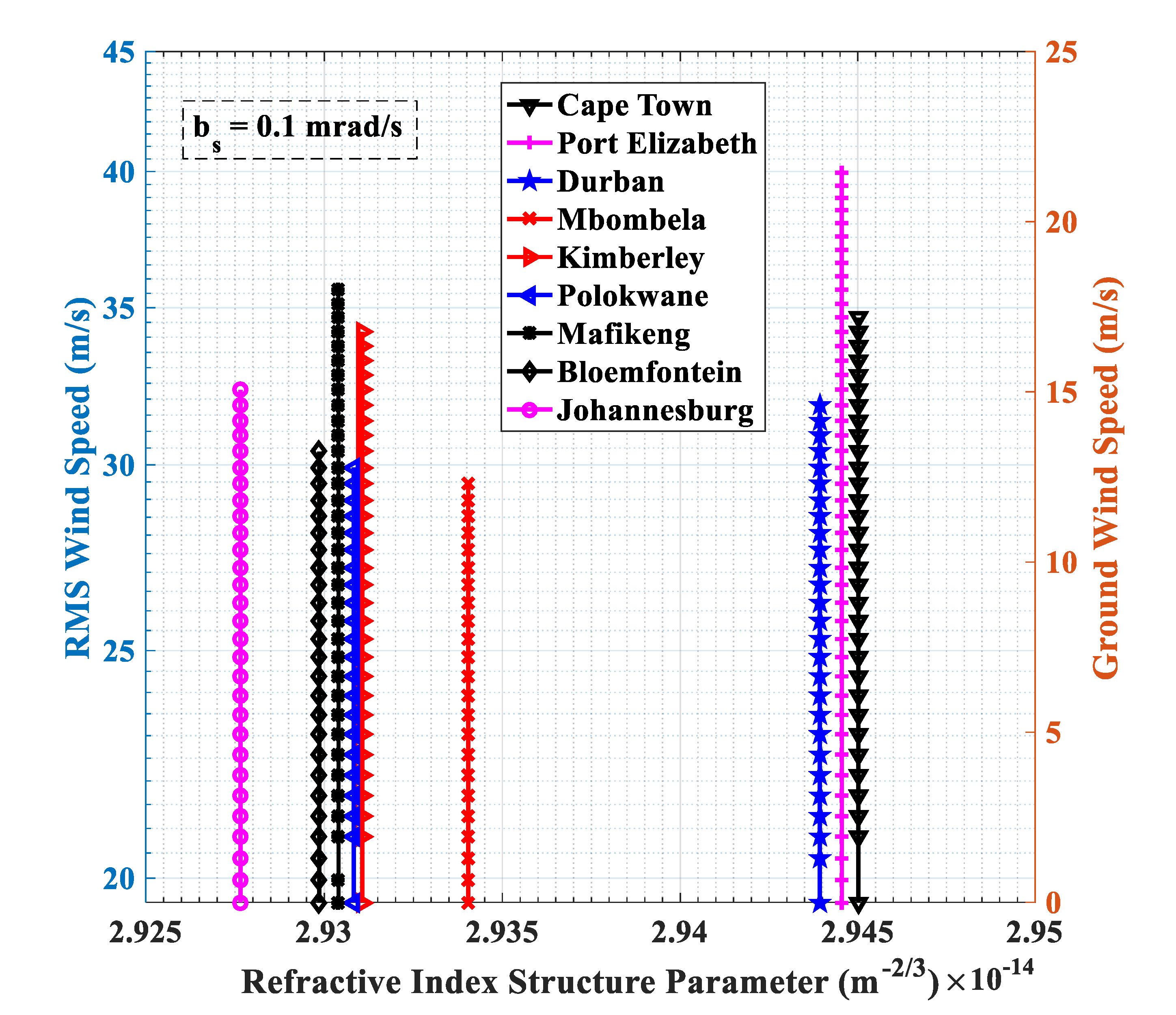
- Computation of the scintillation profile for Gaussian beam FSOC signals in the nine cities under investigation based on the zero inner scale and infinite outer scale model and finite inner and finite outer scale model. To the best of our knowledge, the computation of the scintillation profile for Gaussian beam FSOC links transmitting at 1550 nm in the cities of interest, while considering periods not exceeded 50%, 99%, 99.9%, and 99.99% of the time have not been reported in open literature.
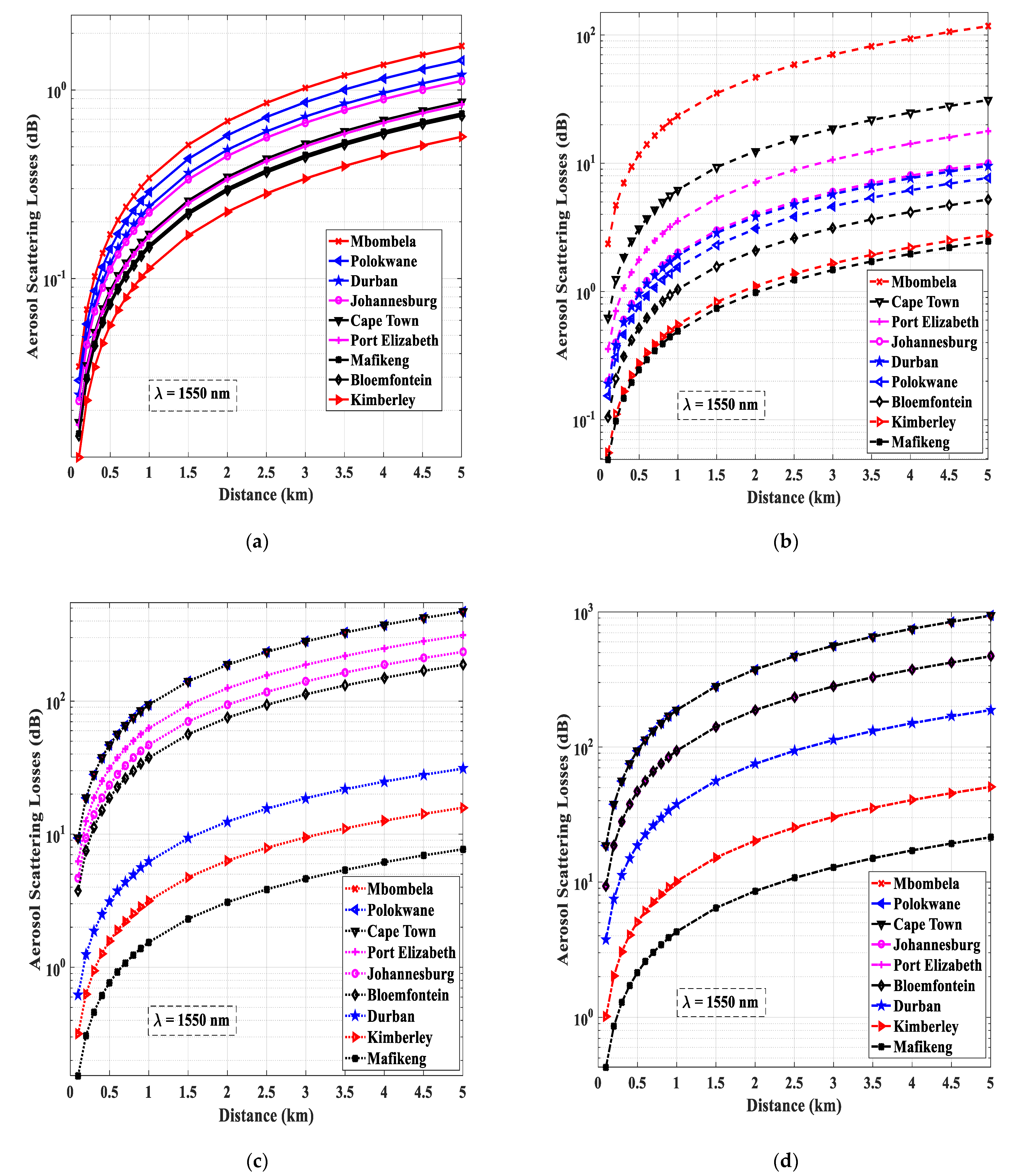
- Aerosol scattering losses over various distances for FSOC links transmitting at 1550 nm with respect to events not exceeded 50%, 99%, 99.9%, and 99.99% of the time, for nine major locations in South Africa, are investigated.
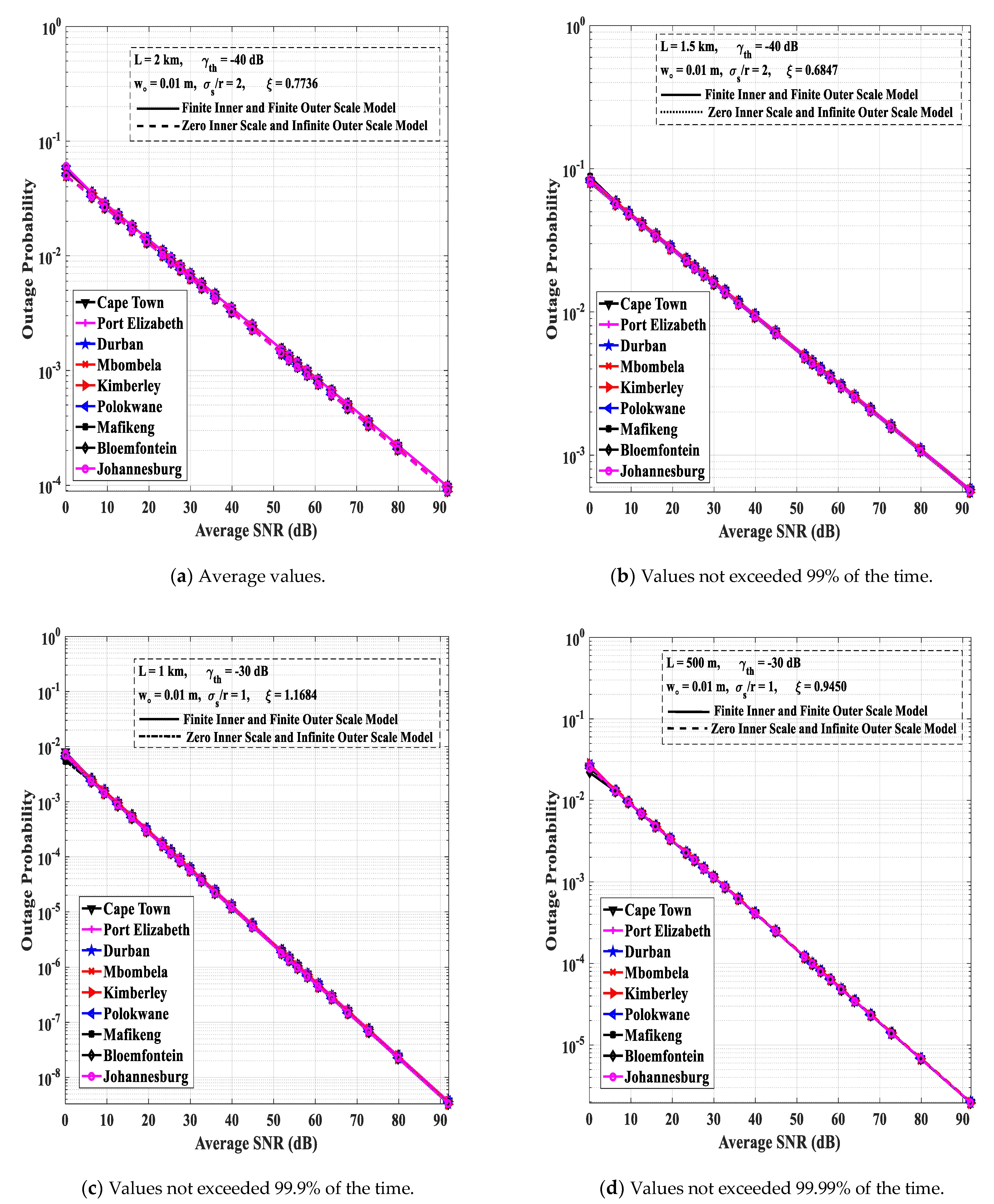
- Outage probabilities of Gaussian beam FSOC links based on the aforementioned scintillation models, while taking into account the effect of pointing errors for events not exceeding the previously mentioned time intervals, are presented for various locations of interest.
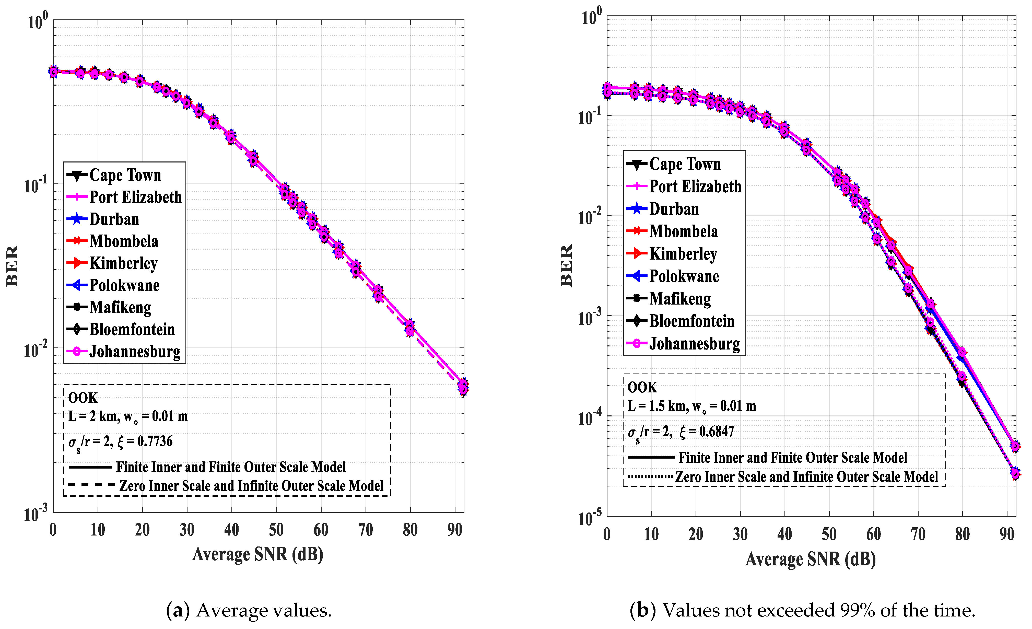
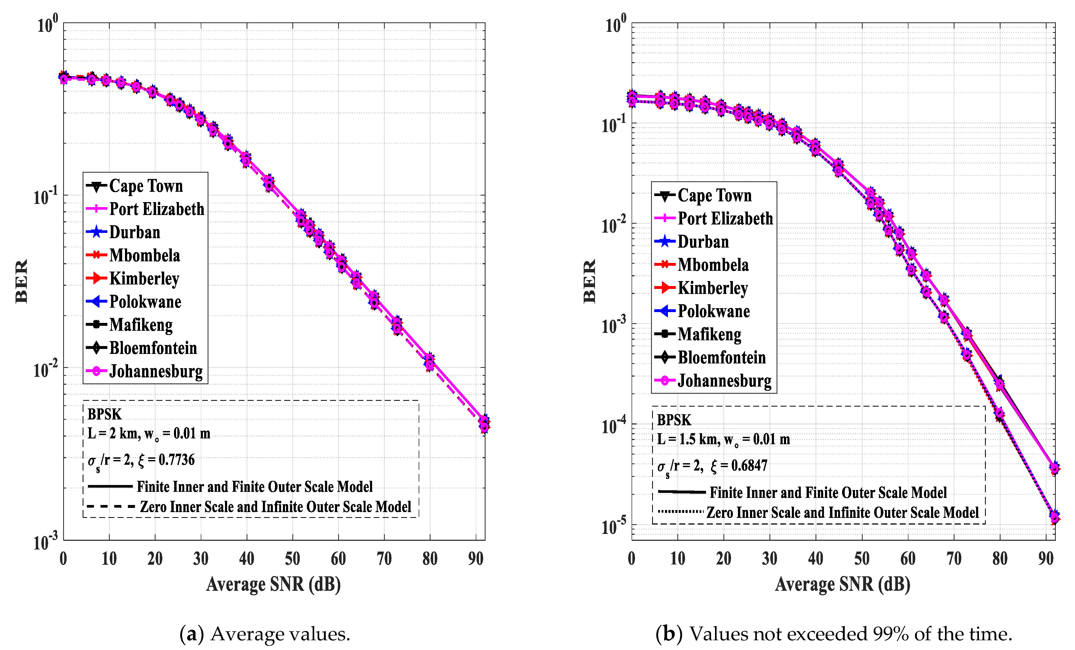
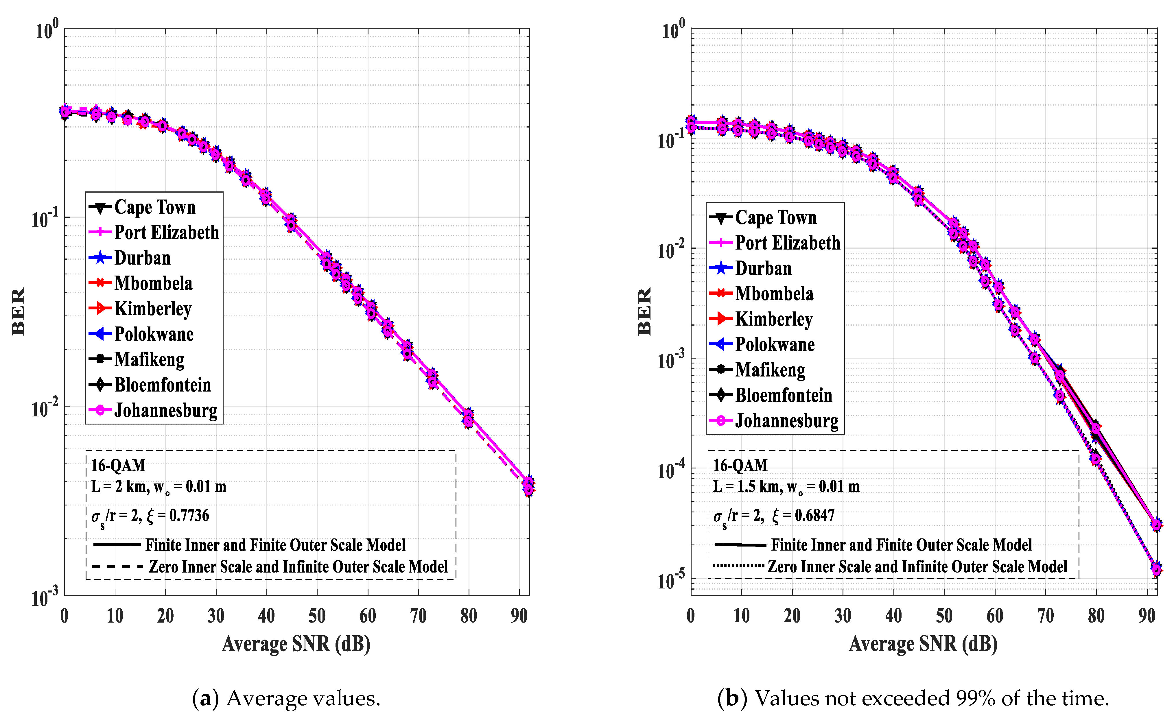
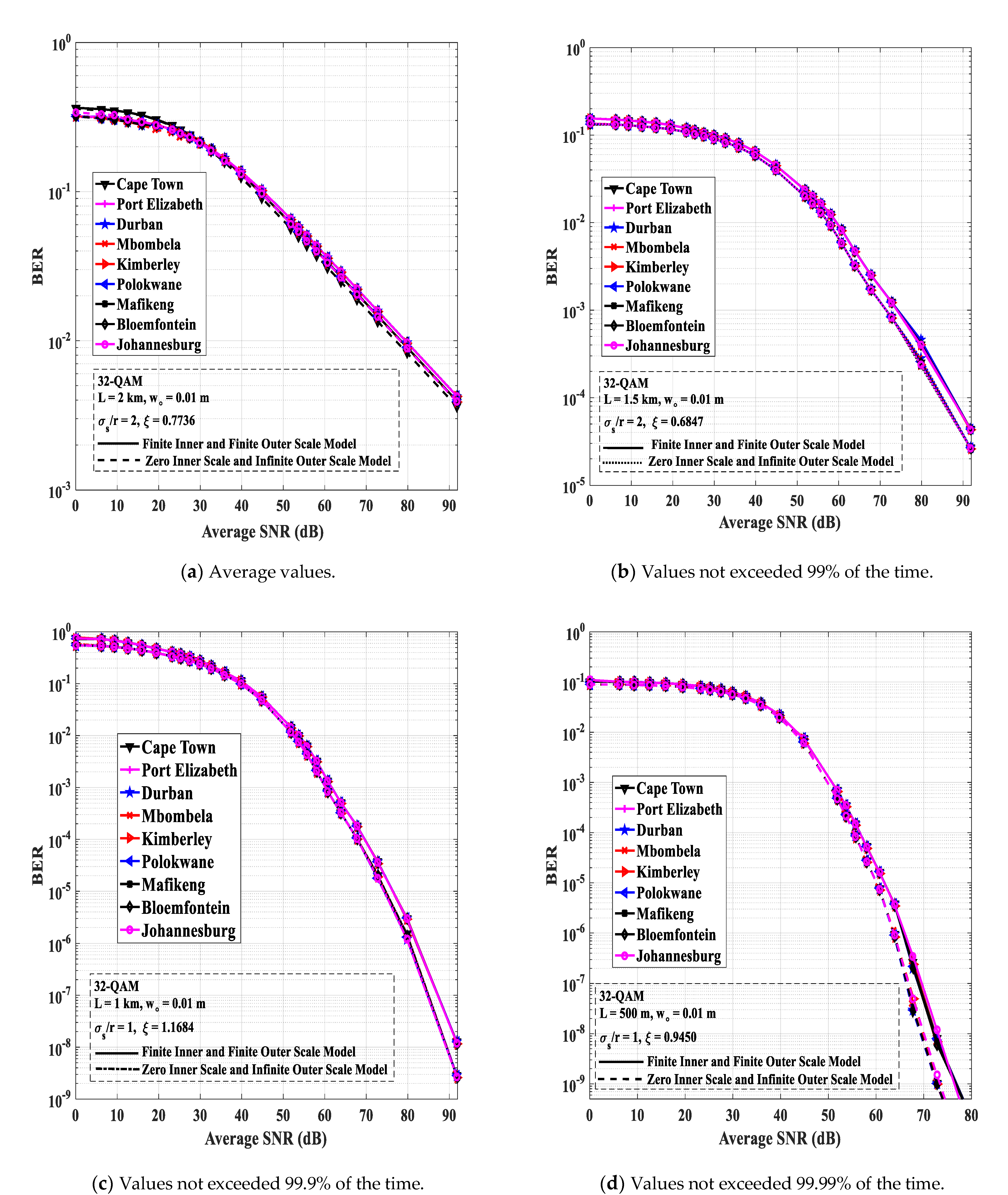
- Analysis of the bit error rate (BER) performance for intensity modulation and direct detection (IM/DD) avalanche photodiode (APD) FSOC systems transmitting at 1550 nm and based on OOK, BPSK, square, and rectangular SIM-QAM schemes during weak, moderate, and strong atmospheric turbulence, with regards to average weather measurements and events not exceeding 99%, 99.9%, and 99.99% of the time are presented.
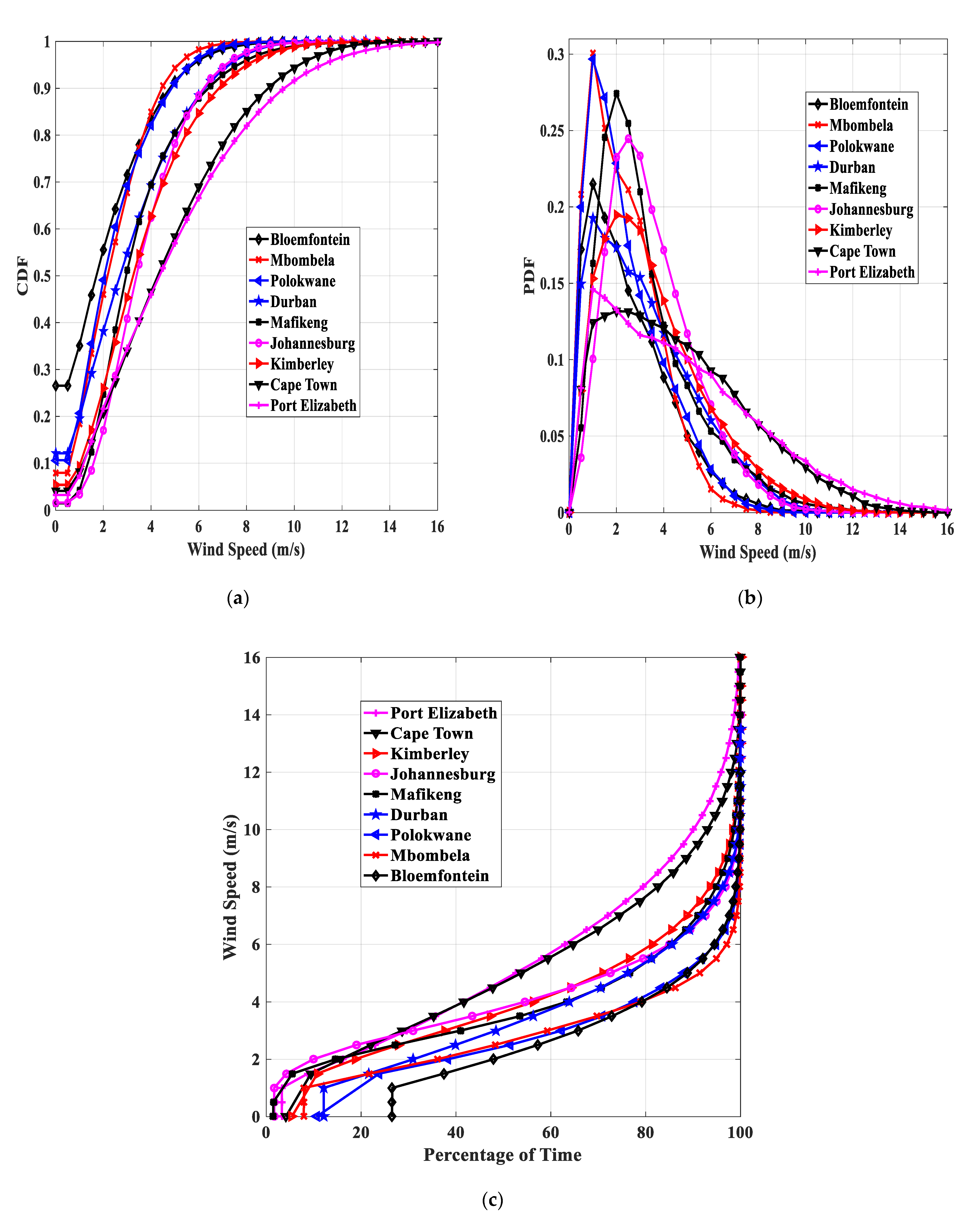
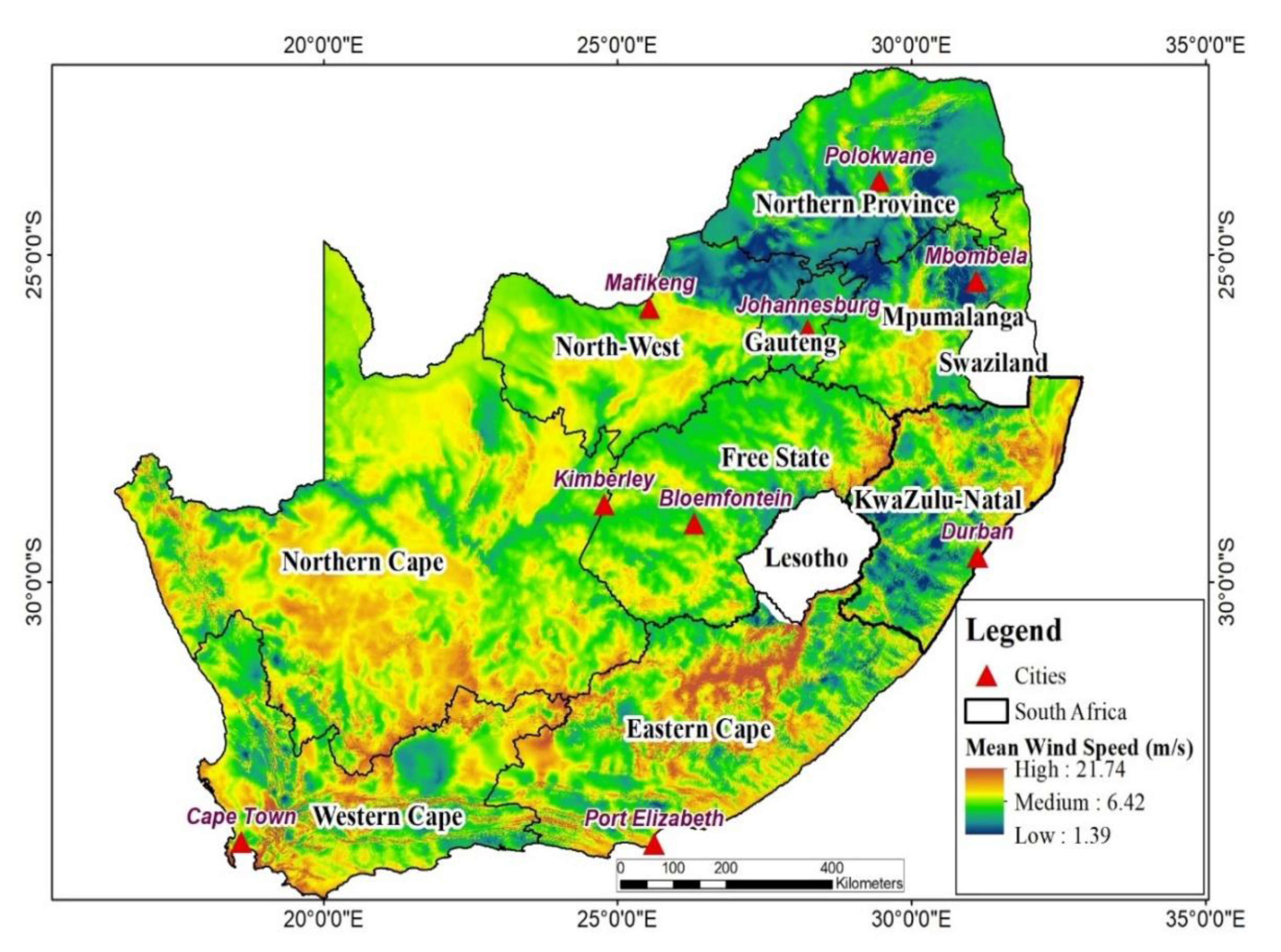
2. Wind Speed Distribution
3. Modified Rytov Theory for Gaussian Beam Waves
3.1. Zero Inner Scale and Infinite Outer Scale Model (Infinite Kolmogorov Inertial Range)
3.2. Finite Inner and Finite Outer Scale Model (Modified Atmospheric Spectrum)
4. Aerosol Scattering Losses
5. Intensity Distribution
6. Outage Probability Analysis
7. Average Bit Error Rate (BER) Analysis
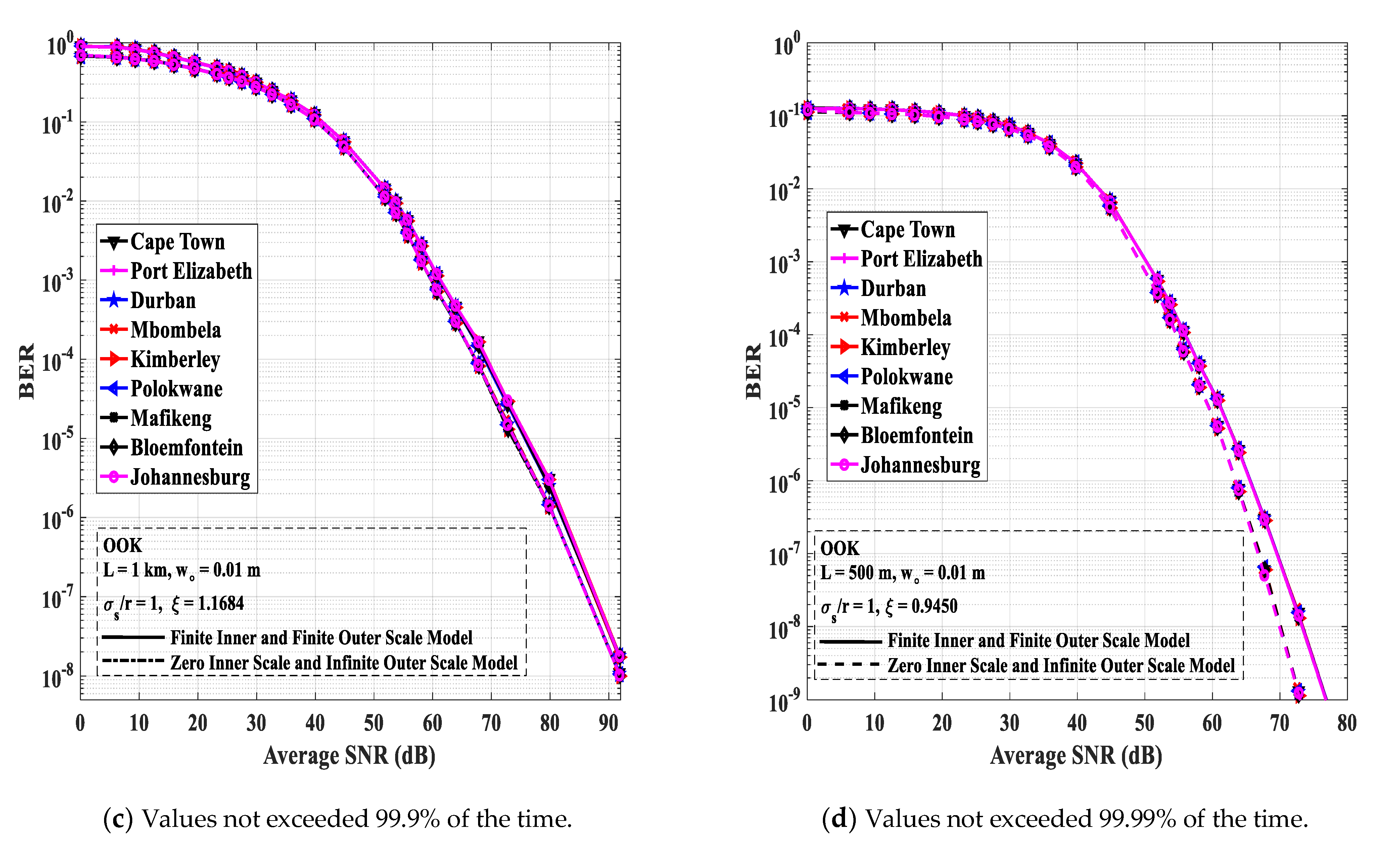
7.1. Return-to-Zero On-Off Keying (RZ-OOK) FSOC Links
- Weak Atmospheric Turbulence
- 2.
- Moderate to Strong Atmospheric Turbulence
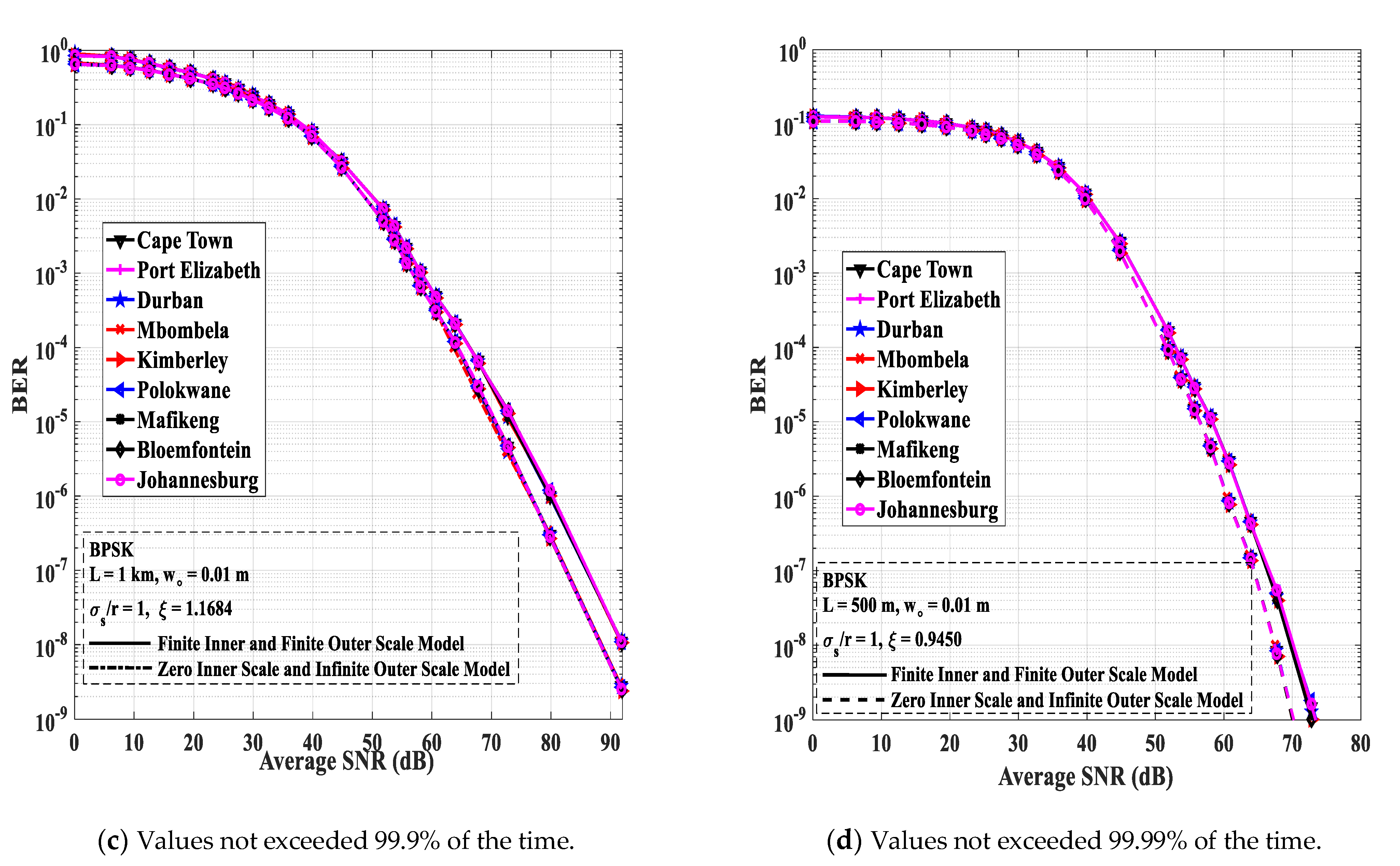
7.2. Binary Phase Shift Keying (BPSK) FSOC Links
- Weak Atmospheric Turbulence
- 2.
- Moderate to Strong Atmospheric Turbulence
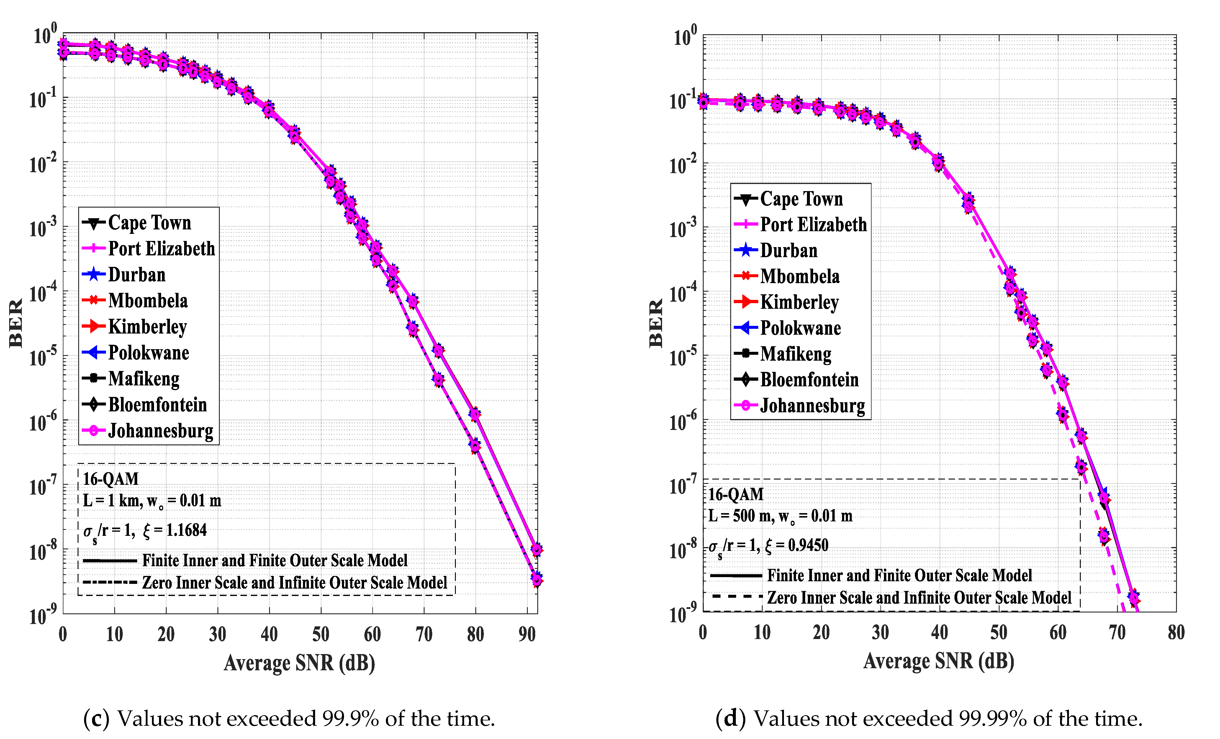
7.3. Quadrature Amplitude Modulation (SIM-QAM) FSOC Links
7.3.1. M-ary Square SIM-QAM FSOC Links
- Weak Atmospheric Turbulence
- 2.
- Moderate to Strong Atmospheric Turbulence
7.3.2. I × J Rectangular QAM FSOC Links
- Weak Atmospheric Turbulence
- 2.
- Moderate to Strong Atmospheric Turbulence
8. Conclusions
Author Contributions
Funding
Institutional Review Board Statement
Data Availability Statement
Acknowledgments
Conflicts of Interest
References
- ITU-R. Detailed Specifications of the Terrestrial Radio Interfaces of International Mobile Telecommunications-2020 (IMT-2020); Rec. ITU-R M.2150-0; M Series; ITU: Geneva, Switzerland, 2022; pp. 1–253. [Google Scholar]
- Erunkulu, O.O.; Zungeru, A.M.; Lebekwe, C.K.; Mosalaosi, M.; Chuma, J.M. 5G mobile communication applications: A survey and comparison of use cases. IEEE Access 2021, 9, 97251–97295. [Google Scholar] [CrossRef]
- Rasheed, I.; Hu, F. Intelligent super-fast Vehicle-to-Everything 5G communications with predictive switching between mmWave and THz links. Veh. Commun. 2021, 27, 100303. [Google Scholar] [CrossRef]
- Lin, Y.B.; Tseng, C.C.; Wang, M.H. Effects of transport network slicing on 5G applications. Future Internet 2021, 13, 69. [Google Scholar] [CrossRef]
- Siriwardhana, Y.; Porambage, P.; Liyanage, M.; Ylianttila, M. A Survey on Mobile Augmented Reality with 5G Mobile Edge Computing: Architectures, Applications, and Technical Aspects. IEEE Commun. Surv. Tutor. 2021, 23, 1160–1192. [Google Scholar] [CrossRef]
- Malik, S.; Sahu, P.K. Free space optics/millimeter-wave based vertical and horizontal terrestrial backhaul network for 5G. Opt. Commun. 2020, 459, 125010. [Google Scholar] [CrossRef]
- Palliyembil, V.; Vellakudiyan, J.; Muthuchidambaranathan, P. Performance analysis of RF-FSO communication systems over the Málaga distribution channel with pointing error. Optik 2021, 247, 167891. [Google Scholar] [CrossRef]
- Garlinska, M.; Pregowska, A.; Masztalerz, K.; Osial, M. From mirrors to free-space optical communication—historical aspects in data transmission. Future Internet 2020, 12, 179. [Google Scholar] [CrossRef]
- Kolawole, O.; Afullo, T.; Mosalaosi, M. Estimation of Optical Wireless Communication Link Availability Using Meteorological Visibility Data for Major Locations in South Africa. In Proceedings of the 2019 PhotonIcs & Electromagnetics Research Symposium-Spring (PIERS-Spring), Rome, Italy, 17–20 June 2019; pp. 319–325. [Google Scholar]
- Kolawole, O.O.; Afullo, T.J.O.; Mosalaosi, M. Initial Modeling of Atmospheric Turbulence Effect on Optical Wireless Communication Links in South Africa. In Proceedings of the Southern Africa Telecommunication Networks and Applications Conference (SATNAC) 2019, Ballito, KwaZulu-Natal, South Africa, 1–4 September 2019; pp. 68–72. [Google Scholar]
- Kolawole, O.O.; Afullo, T.J.O.; Owolawi, P.A. Performance Analysis of Cross M-QAM over Weak Atmospheric Turbulence Channel. In Proceedings of the Southern Africa Telecommunication Networks and Applications Conference (SATNAC) 2016, George, Western Cape, South Africa, 4–7 September 2016; pp. 80–84. [Google Scholar]
- Dordová, L.; Wilfert, O. Calculation and comparison of turbulence attenuation by different methods. Radioengineering 2010, 19, 162–167. [Google Scholar]
- Dubey, D.; Prajapati, Y.K.; Tripathi, R. Error performance analysis of PPM-and FSK-based hybrid modulation scheme for FSO satellite downlink. Opt. Quant. Elect. 2020, 52, 286. [Google Scholar]
- AlQuwaiee, H.; Yang, H.; Alouini, M. On the Asymptotic Capacity of Dual-Aperture FSO Systems with Generalized Pointing Error Model. IEEE Trans. Wirel. Commun. 2016, 15, 6502–6512. [Google Scholar] [CrossRef] [Green Version]
- Borah, D.K.; Voelz, D.G. Pointing Error Effects on Free-Space Optical Communication Links in the Presence of Atmospheric Turbulence. J. Lightwave Tech. 2009, 27, 3965–3973. [Google Scholar] [CrossRef]
- Dubey, D.; Prajapati, Y.K.; Tripathi, R. Optimization of hybrid high-throughput MIMO system with misaligned FSO link under varied weather. Opt. Eng. 2021, 60, 086106. [Google Scholar] [CrossRef]
- Farid, A.A.; Hranilovic, S. Outage Capacity Optimization for Free-Space Optical Links with Pointing Errors. J. Lightwave Tech. 2007, 25, 1702–1710. [Google Scholar] [CrossRef] [Green Version]
- Trung, H.D.; Tuan, D.T.; Pham, A.T. Pointing error effects on performance of free-space optical communication systems using SC-QAM signals over atmospheric turbulence channels. AEU-Int. J. Electron. Commun. 2014, 68, 869–876. [Google Scholar] [CrossRef]
- Ruiz, R.B.; Zambrana, A.G.; Vazquez, B.C.; Vazquez, C.C. Impact of nonzero boresight pointing error on ergodic capacity of MIMO FSO communication systems. Opt. Express 2016, 24, 3513–3534. [Google Scholar] [CrossRef] [PubMed]
- Liu, H.; Liao, R.; Wei, Z.; Hou, Z.; Qiao, Y. BER analysis of a hybrid modulation scheme based on PPM and MSK subcarrier intensity modulation. IEEE Photonics J. 2015, 7, 7201510. [Google Scholar] [CrossRef]
- Sharma, K.; Grewal, S.K. Performance assessment of hybrid PPM–BPSK–SIM based FSO communication system using time and wavelength diversity under variant atmospheric turbulence. Opt. Quant. Elect. 2020, 52, 430. [Google Scholar] [CrossRef]
- Singya, P.K.; Shaik, P.; Kumar, N.; Bhatia, V.; Alouini, M.S. A Survey on Higher-Order QAM Constellations: Technical Challenges, Recent Advances, and Future Trends. IEEE Open J. Commun. Soc. 2021, 2, 617–655. [Google Scholar] [CrossRef]
- Vu, B.T.; Truong, C.T.; Pham, A.T.; Dang, N.T. Performance of rectangular QAM/FSO systems using APD receiver over atmospheric turbulence channels. In Proceedings of the TENCON 2012 IEEE Region 10 Conference, Cebu, Philippines, 19–22 November 2012; pp. 1–5. [Google Scholar]
- Vu, B.T.; Dang, N.T.; Thang, T.C.; Pham, A.T. Bit error rate analysis of rectangular QAM/FSO systems using an APD receiver over atmospheric turbulence channels. J. Opt. Commun. Netw. 2013, 5, 437–446. [Google Scholar] [CrossRef] [Green Version]
- Sprung, D.; van Eijk, A.M.J.; Sucher, E.; Eisele, C.; Seiffer, D.; Stein, K. First results on the Experiment FESTER on optical turbulence over False Bay South Africa: Dependencies and consequences. In Proceedings of the Volume 10002 SPIE Remote Sensing, Edinburgh, UK, 26–29 September 2016; pp. 1–9. [Google Scholar]
- Sprung, D.; van Eijk, A.M.J.; Ullwer, C.; Gunter, W.; Eisele, C.; Seiffer, D.; Sucher, E.; Stein, K. Optical turbulence in the coastal area over False Bay, South Africa: Comparison of measurements and modeling results. In Proceedings of the Volume 10787 SPIE Remote Sensing, Berlin, Germany, 10–13 September 2016; pp. 1–8. [Google Scholar]
- Aly, A.M.; Fayed, H.A.; Ismail, N.E.; Aly, M.H. Plane wave scintillation index in slant path atmospheric turbulence: Closed form expressions for uplink and downlink. Opt. Quant. Elect. 2020, 52, 350. [Google Scholar] [CrossRef]
- Handura, M.; Ndjavera, K.; Nyirenda, C.; Olwal, T.O. Determining the feasibility of free space optical communication in Namibia. Opt. Commun. 2016, 366, 425–430. [Google Scholar] [CrossRef]
- Mohale, J.; Handura, M.R.; Olwal, T.O.; Nyirenda, C.N. Feasibility study of free-space optical communication for South Africa. Opt. Eng. 2016, 55, 056108. [Google Scholar] [CrossRef]
- Mukherjee, A.; Kar, S.; Jain, V.K. Analysis of beam wander effect in high turbulence for FSO communication link. IET Commun. 2018, 12, 2533–2537. [Google Scholar] [CrossRef]
- Abaza, M.; Mesleh, R.; Mansour, A.; el-Hadi, A. Performance analysis of MISO multi-hop FSO links over log-normal channels with fog and beam divergence attenuations. Opt. Commun. 2015, 334, 247–252. [Google Scholar] [CrossRef]
- Kolawole, O.O.; Afullo, T.J.; Mosalaosi, M. Initial Estimation of Scintillation Effect on Free Space Optical Links in South Africa. In Proceedings of the 2019 IEEE AFRICON Conference, Accra, Ghana, 25–27 September 2019. [Google Scholar]
- Shahiduzzaman, K.; Haider, M.F.; Karmaker, B.K. Terrestrial free space optical communications in Bangladesh: Transmission channel characterization. Int. J. Electr. Comput. Eng. 2019, 9, 3130–3138. [Google Scholar] [CrossRef]
- Global Wind Atlas. Available online: https://globalwindatlas.info/ (accessed on 21 September 2021).
- Karp, S.; Stotts, L.B. Communications in the turbulent channel. In Fundamentals of Electro-Optic Systems Design: Communications, LiDAR, and Imaging; Cambridge University Press: Cambridge, UK, 2013; pp. 179–248. [Google Scholar]
- Stotts, L.B. Optical channel effects. In Free Space Optical Systems Engineering: Design and Analysis; John Wiley & Sons, Inc.: Hoboken, NJ, USA, 2017; pp. 239–295. [Google Scholar]
- Andrews, L.C.; Phillips, R.L.; Crabbs, R.; Wayne, D.; Leclerc, T.; Sauer, P. Atmospheric channel characterization for ORCA testing at NTTR. In Proceedings of the Atmospheric and Oceanic Propagation of Electromagnetic Waves IV, San Francisco, CA, USA, 26 February 2010. [Google Scholar]
- Andrews, L.C.; Phillips, R.L. Laser Beam Propagation through Random Media, 2nd ed.; SPIE Press: Bellingham, WA, USA, 2005; pp. 1–773. [Google Scholar]
- Andrews, L.C. Field Guide to Atmospheric Optics, 2nd ed.; SPIE Press: Bellingham, WA, USA, 2004; pp. 1–90. [Google Scholar]
- Engelbrecht, C.J.; Engelbrecht, F.A. Shifts in Köppen-Geiger climate zones over southern Africa in relation to key global temperature goals. Theor. Appl. Climatol. 2016, 123, 247–261. [Google Scholar] [CrossRef]
- Tyson, P.D.; Preston-Whyte, R.A. Atmospheric circulation and weather over Southern Africa. In Weather and Climate of Southern Africa, 2nd ed.; Oxford University Press Southern Africa: Cape Town, South Africa, 2000; pp. 176–217. [Google Scholar]
- Kolawole, O.O.; Afullo, T.J.O.; Mosalaosi, M. Terrestrial free space optical communication systems availability based on meteorological visibility data for South Africa. SAIEE Afr. Res. J. 2022, 113, 20–36. [Google Scholar] [CrossRef]
- Prokeš, A. Modeling of atmospheric turbulence effect on terrestrial FSO link. Radioengineering 2009, 18, 42–47. [Google Scholar]
- Andrews, L.C.; Phillips, R.L.; Hopen, C.Y. Laser Beam Scintillation with Applications, 1st ed.; SPIE Press: Bellingham, WA, USA, 2001; pp. 1–368. [Google Scholar]
- Katsilieris, T.D.; Latsas, G.P.; Nistazakis, H.E.; Tombras, G.S. An accurate computational tool for performance estimation of FSO communication links over weak to strong atmospheric turbulent channels. Computation 2017, 5, 18. [Google Scholar] [CrossRef] [Green Version]
- Recolons, J.; Andrews, L.C.; Phillips, R.L. Analysis of beam wander effects for a horizontal-path propagating Gaussian-beam wave: Focused beam case. Opt. Eng. 2007, 46, 086002. [Google Scholar]
- Prokes, A. Atmospheric effects on availability of free space optics systems. Opt. Eng. 2009, 48, 066001. [Google Scholar] [CrossRef] [Green Version]
- Kim, I.I.; McArthur, B.; Korevaar, E.J. Comparison of laser beam propagation at 785 nm and 1550 nm in fog and haze for optical wireless communications. In Proceedings of the SPIE 4214 Optical Wireless Communications III, Boston, MA, USA, 6 February 2001; pp. 26–37. [Google Scholar]
- Ijaz, M. Experimental Characterisation and Modelling of Atmospheric Fog and Turbulence in FSO. Ph.D. Thesis, Northumbria University, Faculty Eng. Env., Newcastle upon Tyne, UK, 2013. [Google Scholar]
- Ijaz, M.; Ghassemlooy, Z.; Pesek, J.; Fiser, O.; Le Minh, H.; Bentley, E. Modeling of fog and smoke attenuation in free space optical communications link under controlled laboratory conditions. J. Lightwave Tech. 2013, 31, 1720–1726. [Google Scholar] [CrossRef]
- Luong, D.A.; Thang, T.C.; Pham, A.T. Effect of avalanche photodiode and thermal noises on the performance of binary phase-shift keying subcarrier-intensity modulation/free-space optical systems over turbulence channels. IET Commun. 2013, 7, 738–744. [Google Scholar] [CrossRef] [Green Version]
- Andrews, L.C.; Phillips, R.L. Field Guide to Probability, Random Processes, and Random Data Analysis, 1st ed.; SPIE Press: Bellingham, WA, USA, 2012; pp. 1–89. [Google Scholar]
- Wolfram Research Inc. 2008. Available online: https://functions.wolfram.com/PDF/MeijerG.pdf (accessed on 9 August 2021).
- Andrews, L.C. Field Guide to Special Functions for Engineers, 1st ed.; SPIE Press: Bellingham, WA, USA, 2011; pp. 1–101. [Google Scholar]
- Djordjevic, G.T.; Petkovic, M.I.; Cvetkovic, A.M.; Karagiannidis, G.K. Mixed RF/FSO Relaying With Outdated Channel State Information. IEEE J. Sel. Areas Commun. 2015, 33, 1935–1948. [Google Scholar] [CrossRef]
- Feng, J.; Zhao, X. Performance analysis of OOK-based FSO systems in Gamma–Gamma turbulence with imprecise channel models. Opt. Commun. 2017, 402, 340–348. [Google Scholar] [CrossRef]
- Song, X.; Yang, F.; Cheng, J. Subcarrier BPSK modulated FSO communications with pointing errors. In Proceedings of the 2013 IEEE Wireless Communications and Networking Conference (WCNC), Shanghai, China, 7–10 April 2013; pp. 4261–4265. [Google Scholar]
- Ismail, T.; Leitgeb, E. Performance analysis of SIM-DPSK FSO system over lognormal fading with pointing errors. In Proceedings of the 2016 18th International Conference on Transparent Optical Networks (ICTON), Trento, Italy, 10–14 July 2016; pp. 1–4. [Google Scholar]
- Petković, M.I.; Đorđević, G.T.; Milić, D.N. Average BER performance of SIM-DPSK FSO system with APD receiver. Autom. Control Robot. 2015, 14, 111–121. [Google Scholar]
- Petković, M.I.; Đorđević, G.T.; Milić, D.N. BER performance of IM/DD FSO system with OOK using APD receiver. Radioengineering 2014, 23, 480–487. [Google Scholar]
- Zedini, E.; Ansari, I.S.; Alouini, M.S. Performance Analysis of Mixed Nakagami-m and Gamma–Gamma Dual-Hop FSO Transmission Systems. IEEE Photonics J. 2014, 7, 7900120. [Google Scholar] [CrossRef] [Green Version]
- Abramowitz, M.; Stegun, I.A. Handbook of Mathematical Functions with Formulas, Graphs, and Mathematical Tables; US Government Printing Office: Washington, DC, USA, 1964; Volume 55, pp. 1–1062.
- Scheid, F. Schaum’s Outline of Theory and Problems of Numerical Analysis, 2nd ed.; McGraw-Hill: New York, NY, USA, 1989; pp. 1–479. [Google Scholar]
- Mishra, A.; Giri, R.K. Performance Analysis Of Different Modulation Techniques In SIM Based FSO Using Different Receivers Over Turbulent Channel. In Proceedings of the 2018 International Conference on Communication, Computing and Internet of Things (IC3IoT), Chennai, India, 15–17 February 2018; pp. 459–464. [Google Scholar]
- Xu, Z.; Xu, G.; Zheng, Z. BER and Channel Capacity Performance of an FSO Communication System over Atmospheric Turbulence with Different Types of Noise. Sensors 2021, 21, 3454. [Google Scholar] [CrossRef]
- Cho, K.; Yoon, D. On the general BER expression of one- and two-dimensional amplitude modulations. IEEE Trans. Commun. 2002, 50, 1074–1080. [Google Scholar]
- Djordjevic, G.T.; Petkovic, M.I. Average BER performance of FSO SIM-QAM systems in the presence of atmospheric turbulence and pointing errors. J. Mod. Opt. 2015, 63, 715–723. [Google Scholar] [CrossRef]


| City | |
|---|---|
| Cape Town | 42 |
| Port Elizabeth | 69 |
| Durban | 106 |
| Mbombela | 865 |
| Polokwane | 1226 |
| Kimberley | 1196 |
| Mafikeng | 1281 |
| Bloemfontein | 1354 |
| Johannesburg | 1695 |
| City | Ground Wind Speed (m/s) | RMS Wind Speed (m/s) | Propagation Length of 2 km | ||||||
|---|---|---|---|---|---|---|---|---|---|
| Zero Inner Scale and Infinite Outer Scale Model | Finite Inner and Finite Outer Scale Model | ||||||||
| α | β | α | β | ||||||
| Johannesburg | 3.8 | 22.85 | 2.9277 × 10⁻¹⁴ | 0.7488 | 3.3001 | 2.9230 | 0.9311 | 2.6207 | 2.5143 |
| Bloemfontein | 2.2 | 21.43 | 2.9299 × 10⁻¹⁴ | 0.7492 | 3.2985 | 2.9214 | 0.9317 | 2.6192 | 2.5130 |
| Mafikeng | 3.4 | 22.49 | 2.9304 × 10⁻¹⁴ | 0.7494 | 3.2981 | 2.9210 | 0.9318 | 2.6188 | 2.5127 |
| Polokwane | 2.5 | 21.70 | 2.9308 × 10⁻¹⁴ | 0.7494 | 3.2978 | 2.9207 | 0.9319 | 2.6185 | 2.5124 |
| Kimberley | 3.7 | 22.76 | 2.9311 × 10⁻¹⁴ | 0.7495 | 3.2976 | 2.9205 | 0.9320 | 2.6184 | 2.5123 |
| Mbombela | 2.6 | 21.78 | 2.9340 × 10⁻¹⁴ | 0.7501 | 3.2955 | 2.9183 | 0.9328 | 2.6163 | 2.5105 |
| Durban | 3.1 | 22.23 | 2.9439 × 10⁻¹⁴ | 0.7521 | 3.2884 | 2.9110 | 0.9354 | 2.6096 | 2.5047 |
| Port Elizabeth | 4.8 | 23.75 | 2.9446 × 10⁻¹⁴ | 0.7522 | 3.2879 | 2.9106 | 0.9356 | 2.6092 | 2.5044 |
| Cape Town | 4.7 | 23.66 | 2.9450 × 10⁻¹⁴ | 0.7523 | 3.2876 | 2.9102 | 0.9357 | 2.6089 | 2.5041 |
| City | Ground Wind Speed (m/s) | RMS Wind Speed (m/s) | Propagation Length of 1.5 km | ||||||
|---|---|---|---|---|---|---|---|---|---|
| Zero Inner Scale and Infinite Outer Scale Model | Finite Inner and Finite Outer Scale Model | ||||||||
| α | β | α | β | ||||||
| Johannesburg | 9.3 | 27.87 | 2.9277 × 10⁻¹⁴ | 0.4775 | 4.8389 | 4.4556 | 0.5947 | 3.8983 | 3.7156 |
| Bloemfontein | 8.0 | 26.67 | 2.9299 × 10⁻¹⁴ | 0.4778 | 4.8360 | 4.4527 | 0.5951 | 3.8957 | 3.7133 |
| Mafikeng | 10.5 | 28.99 | 2.9304 × 10⁻¹⁴ | 0.4779 | 4.8353 | 4.4520 | 0.5952 | 3.8951 | 3.7128 |
| Polokwane | 7.6 | 26.30 | 2.9308 × 10⁻¹⁴ | 0.4779 | 4.8347 | 4.4515 | 0.5953 | 3.8946 | 3.7123 |
| Kimberley | 10.6 | 29.08 | 2.9311 × 10⁻¹⁴ | 0.4780 | 4.8344 | 4.4511 | 0.5953 | 3.8943 | 3.7121 |
| Mbombela | 6.9 | 25.65 | 2.9340 × 10⁻¹⁴ | 0.4784 | 4.8305 | 4.4473 | 0.5959 | 3.8909 | 3.7090 |
| Durban | 9.4 | 27.96 | 2.9439 × 10⁻¹⁴ | 0.4799 | 4.8175 | 4.4346 | 0.5978 | 3.8795 | 3.6989 |
| Port Elizabeth | 14.5 | 32.76 | 2.9446 × 10⁻¹⁴ | 0.4800 | 4.8167 | 4.4338 | 0.5979 | 3.8788 | 3.6983 |
| Cape Town | 12.7 | 31.05 | 2.9450 × 10⁻¹⁴ | 0.4800 | 4.8161 | 4.4332 | 0.5980 | 3.8783 | 3.6978 |
| City | Ground Wind Speed (m/s) | RMS Wind Speed (m/s) | Propagation Length of 1 km | ||||||
|---|---|---|---|---|---|---|---|---|---|
| Zero Inner Scale and Infinite Outer Scale Model | Finite Inner and Finite Outer Scale Model | ||||||||
| α | β | α | β | ||||||
| Johannesburg | 11.4 | 29.83 | 2.9277 × 10⁻¹⁴ | 0.2362 | 9.2025 | 8.6921 | 0.2956 | 7.4062 | 7.0664 |
| Bloemfontein | 10.1 | 28.61 | 2.9299 × 10⁻¹⁴ | 0.2364 | 9.1962 | 8.6859 | 0.2959 | 7.4009 | 7.0615 |
| Mafikeng | 13.2 | 31.53 | 2.9304 × 10⁻¹⁴ | 0.2364 | 9.1946 | 8.6844 | 0.2959 | 7.3996 | 7.0603 |
| Polokwane | 9.3 | 27.87 | 2.9308 × 10⁻¹⁴ | 0.2365 | 9.1934 | 8.6832 | 0.2960 | 7.3986 | 7.0593 |
| Kimberley | 13.0 | 31.34 | 2.9311 × 10⁻¹⁴ | 0.2365 | 9.1927 | 8.6826 | 0.2960 | 7.3980 | 7.0588 |
| Mbombela | 8.5 | 27.13 | 2.9340 × 10⁻¹⁴ | 0.2367 | 9.1841 | 8.6743 | 0.2963 | 7.3909 | 7.0522 |
| Durban | 11 | 29.46 | 2.9439 × 10⁻¹⁴ | 0.2375 | 9.1557 | 8.6469 | 0.2973 | 7.3673 | 7.0304 |
| Port Elizabeth | 17.2 | 35.33 | 2.9446 × 10⁻¹⁴ | 0.2376 | 9.1539 | 8.6451 | 0.2973 | 7.3658 | 7.0290 |
| Cape Town | 14.7 | 32.95 | 2.9450 × 10⁻¹⁴ | 0.2376 | 9.1526 | 8.6439 | 0.2974 | 7.3647 | 7.0280 |
| City | Ground Wind Speed (m/s) | RMS Wind Speed (m/s) | Propagation Length of 500 m | ||||||
|---|---|---|---|---|---|---|---|---|---|
| Zero Inner Scale and Infinite Outer Scale Model | Finite Inner and Finite Outer Scale Model | ||||||||
| α | β | α | β | ||||||
| Johannesburg | 12.7 | 31.05 | 2.9277 × 10⁻¹⁴ | 0.0672 | 30.927 | 29.602 | 0.0834 | 24.755 | 24.182 |
| Bloemfontein | 11.2 | 29.64 | 2.9299 × 10⁻¹⁴ | 0.0673 | 30.904 | 29.580 | 0.0835 | 24.736 | 24.164 |
| Mafikeng | 16.3 | 34.47 | 2.9304 × 10⁻¹⁴ | 0.0673 | 30.898 | 29.575 | 0.0835 | 24.732 | 24.160 |
| Polokwane | 10.4 | 28.89 | 2.9308 × 10⁻¹⁴ | 0.0673 | 30.894 | 29.571 | 0.0835 | 24.728 | 24.156 |
| Kimberley | 14.6 | 32.85 | 2.9311 × 10⁻¹⁴ | 0.0673 | 30.891 | 29.568 | 0.0835 | 24.726 | 24.154 |
| Mbombela | 10.2 | 28.71 | 2.9340 × 10⁻¹⁴ | 0.0674 | 30.860 | 29.539 | 0.0836 | 24.701 | 24.130 |
| Durban | 12.1 | 30.49 | 2.9439 × 10⁻¹⁴ | 0.0676 | 30.758 | 29.440 | 0.0839 | 24.619 | 24.050 |
| Port Elizabeth | 19.7 | 37.73 | 2.9446 × 10⁻¹⁴ | 0.0676 | 30.752 | 29.434 | 0.0839 | 24.614 | 24.045 |
| Cape Town | 15.9 | 34.09 | 2.9450 × 10⁻¹⁴ | 0.0676 | 30.747 | 29.430 | 0.0839 | 24.610 | 24.041 |
| FSOC Link Parameters | |
|---|---|
| Light Source | Laser |
| Wavelength | 1550 nm |
| Transmit Power | 20 dBm |
| Receiver Sensitivity | −40 dBm |
| Receiver Aperture Diameter | 10 cm |
| Eye Safety | Class 1M |
| Transmit Beam Divergence Angle | 1.75 mrad |
| Responsivity | 0.5 A/W |
| Bit Rate | 10 Gb/s |
| Detector | Avalanche Photodiode (APD) |
| Boltzmann’s Constant | 1.381 × 10⁻²³ J/K |
| Temperature | 298 K |
| Planck’s Constant | 6.626 × 10⁻³⁴ Js |
| Speed of Light | 3 × 10⁸ m/s |
| APD Load Resistance | 1000 Ω |
| APD Gain | 50 |
| Amplifier Noise Figure | 2 |
| Charge of an Electron | 1.602 × 10⁻¹⁹ C |
| Ionization factor for InGaAs APD | 0.7 |
Publisher’s Note: MDPI stays neutral with regard to jurisdictional claims in published maps and institutional affiliations. |
© 2022 by the authors. Licensee MDPI, Basel, Switzerland. This article is an open access article distributed under the terms and conditions of the Creative Commons Attribution (CC BY) license (https://creativecommons.org/licenses/by/4.0/).
Share and Cite
Kolawole, O.O.; Afullo, T.J.O.; Mosalaosi, M. Analysis of Scintillation Effects on Free Space Optical Communication Links in South Africa. Photonics 2022, 9, 446. https://doi.org/10.3390/photonics9070446
Kolawole OO, Afullo TJO, Mosalaosi M. Analysis of Scintillation Effects on Free Space Optical Communication Links in South Africa. Photonics. 2022; 9(7):446. https://doi.org/10.3390/photonics9070446
Chicago/Turabian StyleKolawole, Olabamidele O., Thomas J. O. Afullo, and Modisa Mosalaosi. 2022. "Analysis of Scintillation Effects on Free Space Optical Communication Links in South Africa" Photonics 9, no. 7: 446. https://doi.org/10.3390/photonics9070446
APA StyleKolawole, O. O., Afullo, T. J. O., & Mosalaosi, M. (2022). Analysis of Scintillation Effects on Free Space Optical Communication Links in South Africa. Photonics, 9(7), 446. https://doi.org/10.3390/photonics9070446