Scale-Aware Network with Scale Equivariance


Abstract
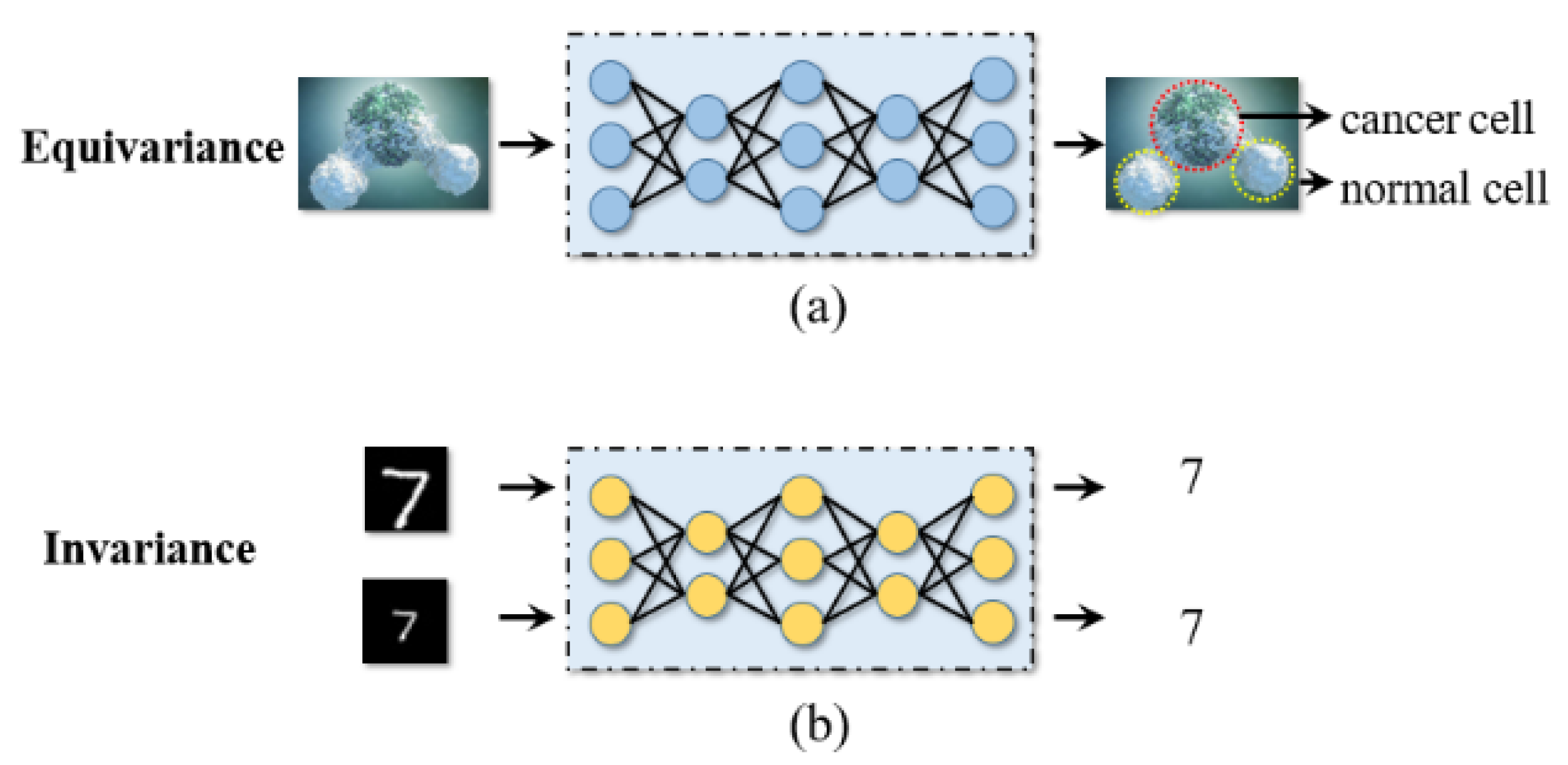
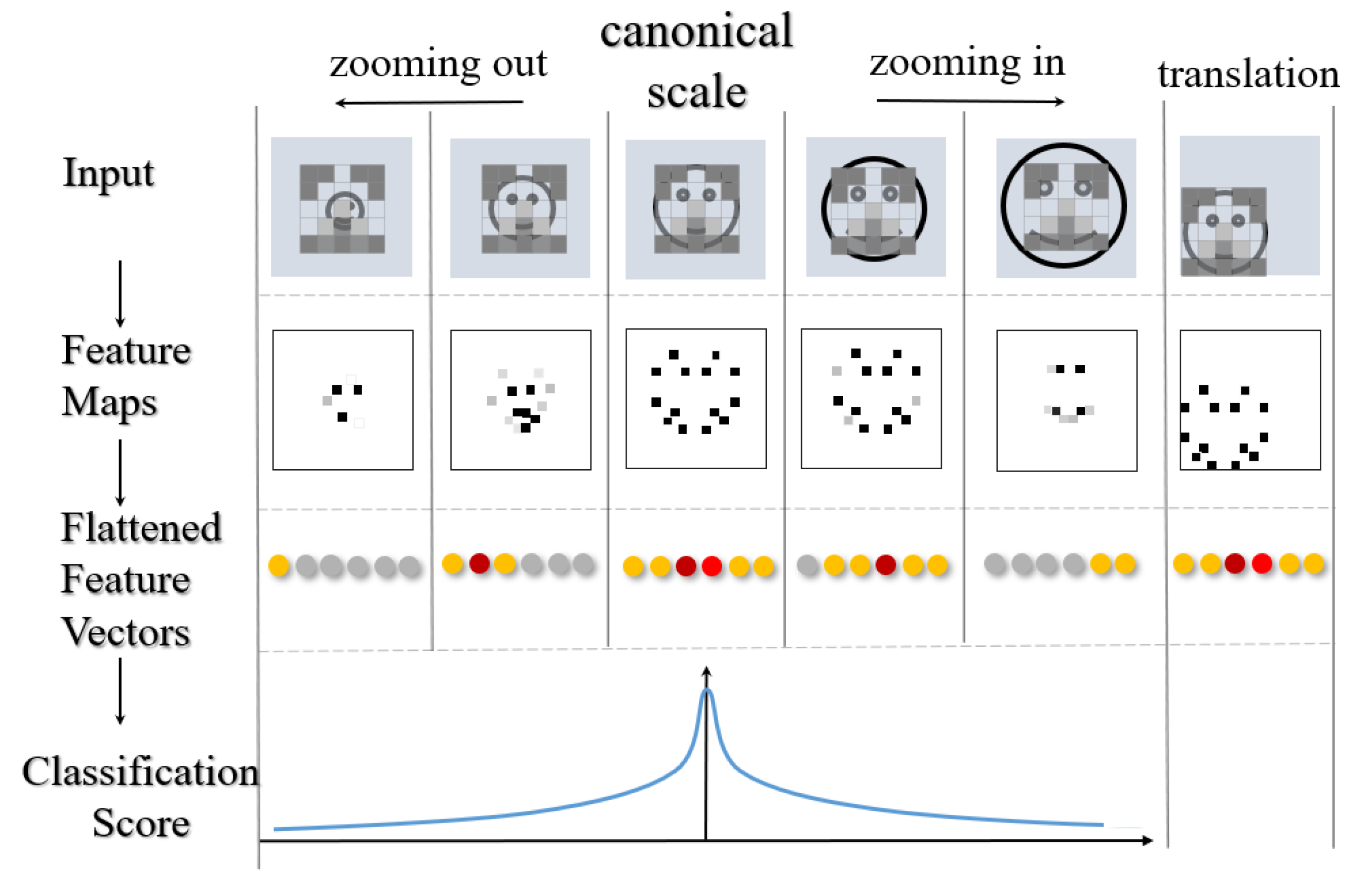
:1. Introduction
2. Related Work
2.1. Multi-Scale Training
2.2. Single-Scale Training
3. Methods
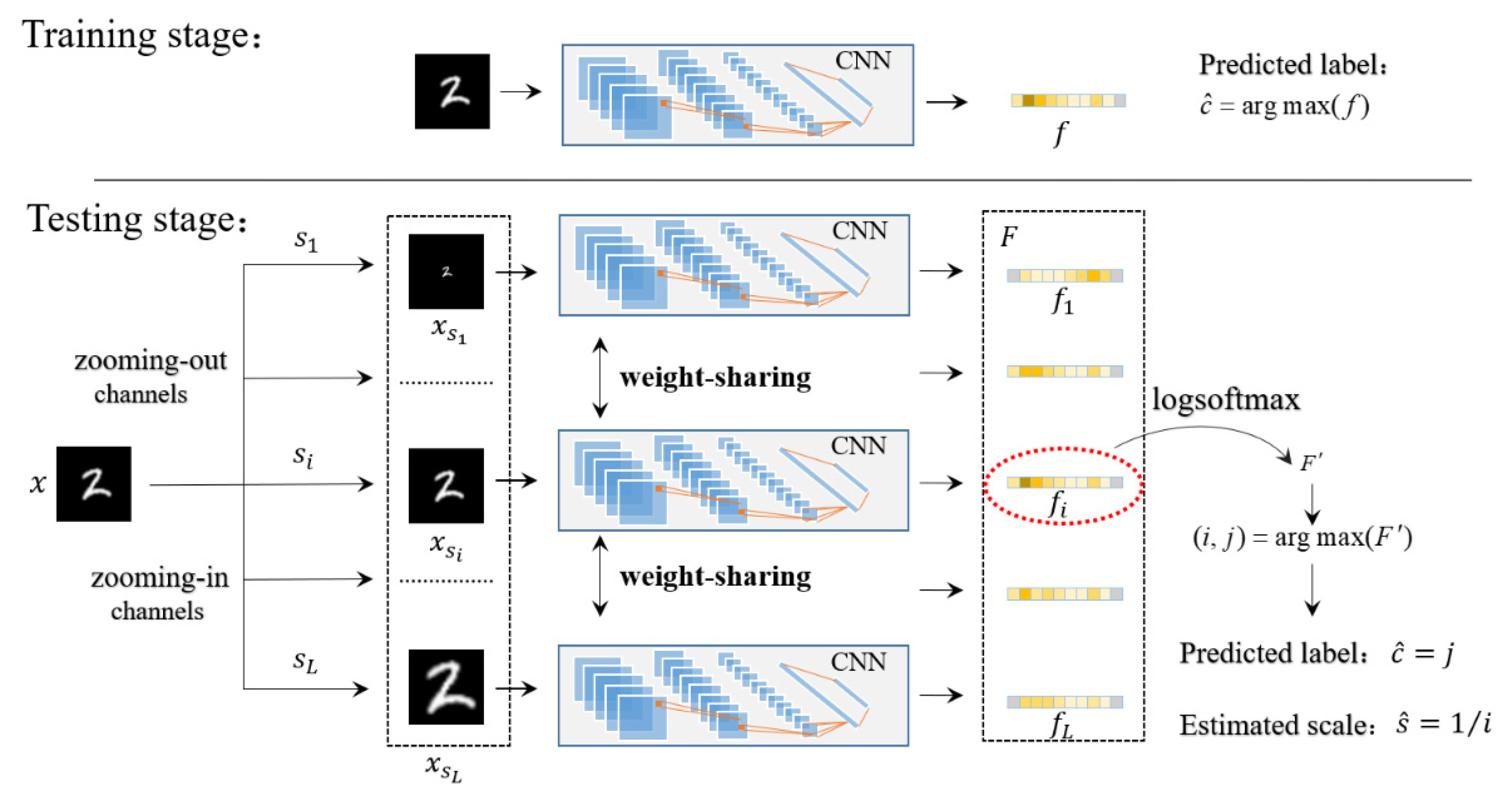
3.1. Training Stage
3.2. Testing Stage
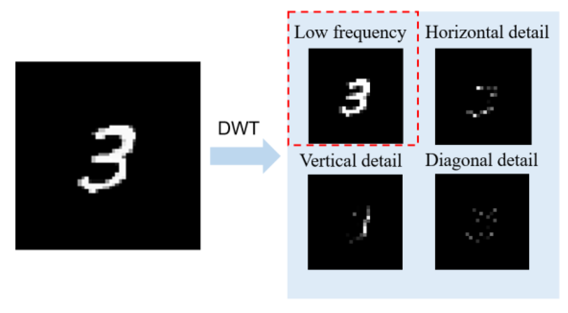
3.2.1. Discrete-Wavelet Transform
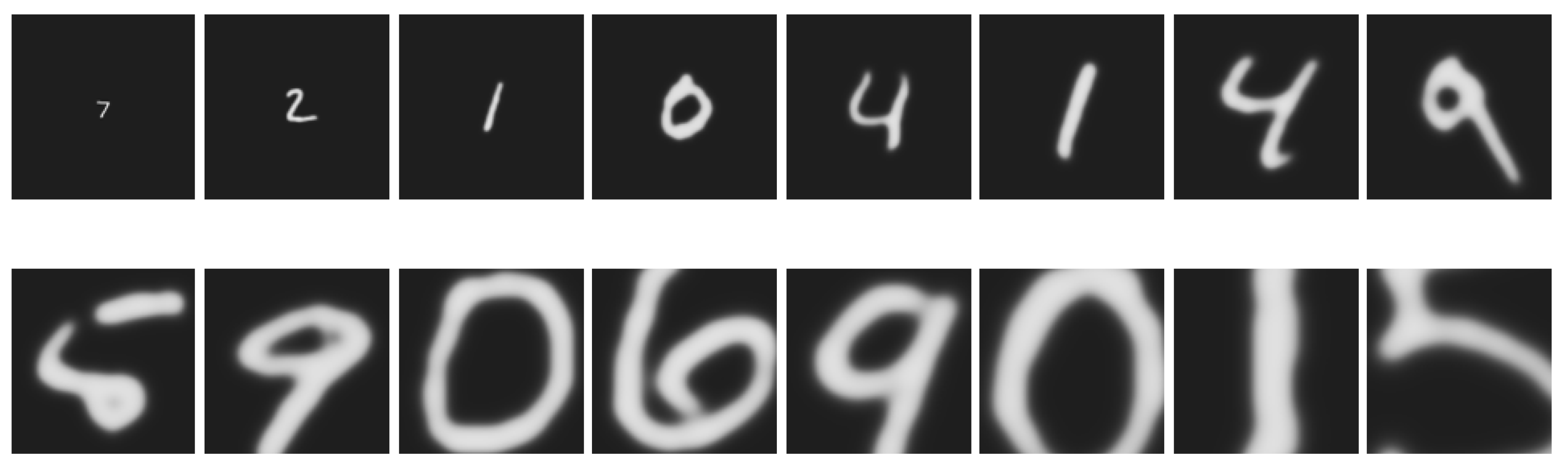
3.2.2. Image Pyramid
3.2.3. Classification and Scale Estimation
| Algorithm 1: Classification and scale estimation algorithm of SA Net |
| Input: Testing set |
| For do Select a sample in order; For do ; ; end // 2-D classification-score matrix ; ; ;…………//label prediction ;…………//scale estimation if then ; end end |
| Output: , |
4. Experiments and Discussion
4.1. Scale Datasets
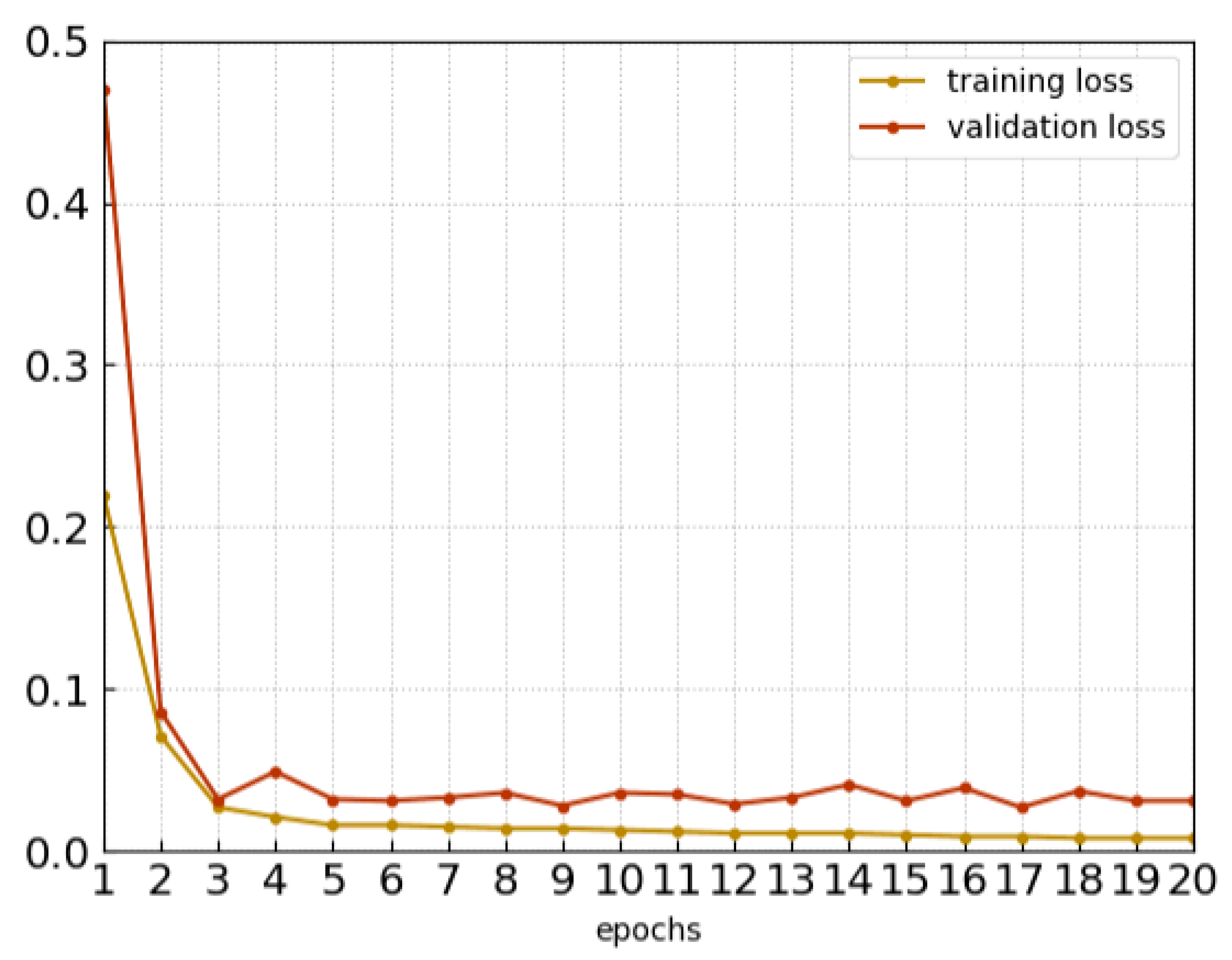
4.2. Implementation Details and Network Parameters
4.3. Classification Experiment
4.4. Scale-Estimation Experiment
4.4.1. Dataset
4.4.2. Receptive Field
- the number of feature channels are 32 and 64, respectively.
- the size of the convolution kernels is three for two blocks.
- the other parameters of the blocks are suitable for the convolution layer.
4.4.3. Experiment Results
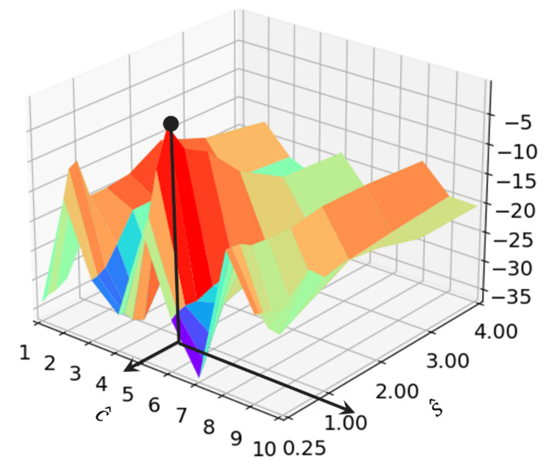
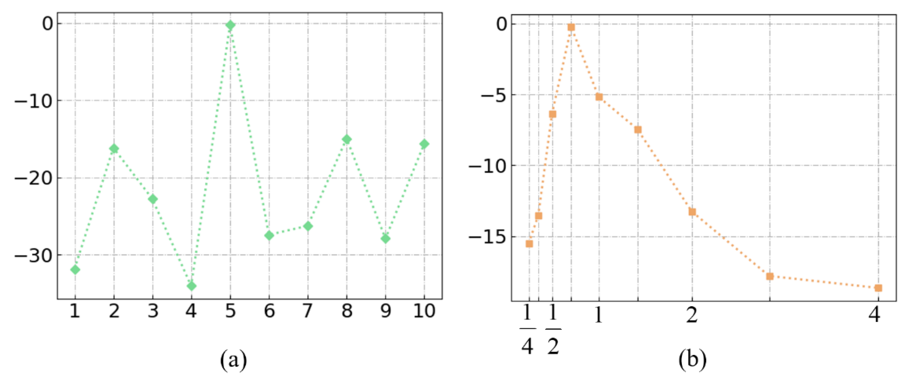
4.4.4. Visualization of Scale Estimation
5. Conclusions
Author Contributions
Funding
Institutional Review Board Statement
Informed Consent Statement
Data Availability Statement
Conflicts of Interest
References
- Krizhevsky, A.; Sutskever, I.; Hinton, G.E. ImageNet Classification with Deep Convolutional Neural Networks. In Proceedings of the 26th Annual Conference on Neural Information Processing Systems (NIPS), Lake Tahoe, NV, USA, 3–6 December 2012; pp. 1106–1114. [Google Scholar]
- Lecun, Y.; Bottou, L.; Bengio, Y.; Haffner, P. Gradient-based learning applied to document recognition. Proc. IEEE 1998, 86, 2278–2324. [Google Scholar] [CrossRef] [Green Version]
- Cohen, T.; Welling, M. Group Equivariant Convolutional Networks. In Proceedings of the 33rd International Conference on Machine Learning (ICML), New York, NY, USA, 19–24 June 2016; pp. 2990–2999. [Google Scholar]
- Marcos, D.; Volpi, M.; Komodakis, N.; Tuia, D. Rotation Equivariant Vector Field Networks. In Proceedings of the IEEE International Conference on Computer Vision (ICCV), Venice, Italy, 22–29 October 2017; pp. 5058–5067. [Google Scholar]
- Lang, M. The Mechanism of Scale-Invariance. arXiv 2021, arXiv:2103.00620v1. [Google Scholar]
- Ma, T.; Gupta, A.; Sabuncu, M.R. Volumetric Landmark Detection with a Multi-Scale Shift Equivariant Neural Network. In Proceedings of the 2020 IEEE 17th International Symposium on Biomedical Imaging (ISBI), Iowa City, IA, USA, 3–7 April 2020; pp. 981–985. [Google Scholar] [CrossRef]
- Azulay, A.; Weiss, Y. Why do deep convolutional networks generalize so poorly to small image transformations? J. Mach. Learn. Res. 2019, 20, 1–25. [Google Scholar]
- Sosnovik, I.; Moskalev, A.; Smeulders, A.W.M. Scale Equivariance Improves Siamese Tracking. In Proceedings of the IEEE Winter Conference on Applications of Computer Vision (WACV), Waikoloa, HI, USA, 3–8 January 2021; pp. 2764–2773. [Google Scholar]
- Wang, Q.; Zheng, Y.; Yang, G.; Jin, W.; Yin, Y. Multi-Scale Rotation-Invariant Convolutional Neural Networks for Lung Texture Classification. IEEE J. Biomed. Health Inform. 2018, 22, 184–195. [Google Scholar] [CrossRef] [PubMed]
- Hanieh, N.; Leili, G.; Shohreh, K. Scale Equivariant CNNs with Scale Steerable Filters. In Proceedings of the International Conference on Machine Vision and Image Processing (MVIP), Tehran, Iran, 18–20 February 2020; pp. 1–5. [Google Scholar]
- Jaderberg, M.; Simonyan, K.; Zisserman, A.; Kavukcuoglu, K. Spatial Transformer Networks. In Proceedings of the Advances in Neural Information Processing Systems, Montreal, QC, Canada, 7–12 December 2015; pp. 2017–2025. [Google Scholar]
- Lindeberg, T. Scale-Covariant and Scale-Invariant Gaussian Derivative Networks. In Proceedings of the 8th International Conference on Scale Space and Variational Methods in Computer Vision (SSVM), Virtual Event, 16–20 May 2021; pp. 3–14. [Google Scholar] [CrossRef]
- Kanazawa, A.; Sharma, A.; Jacobs, D. Locally Scale-Invariant Convolutional Neural Networks. arXiv 2014, arXiv:1412.5104. [Google Scholar]
- Laptev, D.; Savinov, N.; Buhmann, J.M.; Pollefeys, M. TI-POOLING: Transformation-Invariant Pooling for Feature Learning in Convolutional Neural Networks. In Proceedings of the 2016 IEEE Conference on Computer Vision and Pattern Recognition (CVPR), Las Vegas, NV, USA, 27–30 June 2016; pp. 289–297. [Google Scholar] [CrossRef] [Green Version]
- Esteves, C.; Allen-Blanchette, C.; Zhou, X.; Daniilidis, K. Polar Transformer Networks. In Proceedings of the 6th International Conference on Learning Representations (ICLR), Vancouver, BC, Canada, 3 May 2018. [Google Scholar]
- Shorten, C.; Khoshgoftaar, T.M. A survey on Image Data Augmentation for Deep Learning. J. Big Data 2019, 6, 60. [Google Scholar] [CrossRef]
- Marcos, D.; Kellenberger, B.; Lobry, S.; Tuia, D. Scale equivariance in CNNs with vector fields. arXiv 2018, arXiv:1807.11783. [Google Scholar]
- Cohen, T.S.; Welling, M. Steerable CNNs. In Proceedings of the 5th International Conference on Learning Representations (ICLR), Toulon, France, 24–26 April 2017. [Google Scholar]
- Sosnovik, I.; Szmaja, M.; Smeulders, A.W.M. Scale-Equivariant Steerable Networks. In Proceedings of the 8th International Conference on Learning Representations (ICLR), Addis Ababa, Ethiopia, 26–30 April 2020. [Google Scholar]
- Xu, Y.; Xiao, T.; Zhang, J.; Yang, K.; Zhang, Z. Scale-Invariant Convolutional Neural Networks. arXiv 2014, arXiv:1411.6369. [Google Scholar]
- Ghosh, G.; Gupta, A.K. Scale Steerable Filters for Locally Scale-Invariant Convolutional Neural Networks. arXiv 2019, arXiv:1906.03861. [Google Scholar]
- Jansson, Y.; Lindeberg, T. Exploring the ability of CNN s to generalise to previously unseen scales over wide scale ranges. In Proceedings of the 2020 25th International Conference on Pattern Recognition (ICPR), Milan, Italy, 10–15 January 2021; pp. 1181–1188. [Google Scholar] [CrossRef]
- Mallat, S.G. A theory for multiresolution signal decomposition: The wavelet representation. IEEE Trans. Pattern Anal. Mach. Intell. 1989, 11, 674–693. [Google Scholar] [CrossRef] [Green Version]
- Ben Chaabane, C.; Mellouli, D.; Hamdani, T.M.; Alimi, A.M.; Abraham, A. Wavelet Convolutional Neural Networks for Handwritten Digits Recognition. In Proceedings of the 2017 International Conference on Hybrid Intelligent Systems (HIS), Delhi, India, 14–16 December 2017; pp. 305–310. [Google Scholar] [CrossRef]
- Burrus, C.S. Introduction to Wavelets and Wavelet Transforms: A Primer, 1st ed.; Prentice-Hall: Englewood Cliffs, NJ, USA, 1997; pp. 34–36. [Google Scholar]
- Kingma, D.P.; Ba, J. Adam: A Method for Stochastic Optimization. In Proceedings of the 3rd International Conference on Learning Representations (ICLR), San Diego, CA, USA, 7–9 May 2015. [Google Scholar]
- Ioffe, S.; Szegedy, C. Batch Normalization: Accelerating Deep Network Training by Reducing Internal Covariate Shift. In Proceedings of the 32nd International Conference on Machine Learning (ICML), Lille, France, 6–11 July 2015; pp. 448–456. [Google Scholar]
- Xu, L.; Choy, C.-S.; Li, Y.-W. Deep sparse rectifier neural networks for speech denoising. In Proceedings of the IEEE International Workshop on Acoustic Signal Enhancement (IWAENC), Xi’an, China, 13–16 September 2016; pp. 1–5. [Google Scholar]
- Hinton, G.E.; Srivastava, N.; Krizhevsky, A.; Sutskever, I.; Salakhutdinov, R. Improving neural networks by preventing co-adaptation of feature detectors. arXiv 2012, arXiv:1207.0580. [Google Scholar]
- Luo, W.; Li, Y.; Urtasun, R.; Zemel, R. Understanding the Effective Receptive Field in Deep Convolutional Neural Networks. In Proceedings of the 30th International Conference on Neural Information Processing Systems, Barcelona, Spain, 5–10 December 2016. [Google Scholar]
- Zhou, B.; Khosla, A.; Lapedriza, À.; Oliva, A.; Torralba, A. Object Detectors Emerge in Deep Scene CNNs. In Proceedings of the 3rd International Conference on Learning Representations (ICLR), San Diego, CA, USA, 7–9 May 2015. [Google Scholar]
- Xiao, H.; Rasul, K.; Vollgraf, R. Fashion-MNIST: A Novel Image Dataset for Benchmarking Machine Learning Algorithms. arXiv 2017, arXiv:1708.07747. [Google Scholar]
- Yang, Z.; Bai, Y.-M.; Sun, L.-D.; Huang, K.-X.; Liu, J.; Ruan, D.; Li, J.-L. SP-ILC: Concurrent Single-Pixel Imaging, Object Location, and Classification by Deep Learning. Photonics 2021, 8, 400. [Google Scholar] [CrossRef]


| Datasets | Methods | Wavelet Basis | 8 | ||||||||
|---|---|---|---|---|---|---|---|---|---|---|---|
| MNIST Large Scale | CNN | — | 20.86 | 38.67 | 68.35 | 96.60 | 99.38 | 94.98 | 45.83 | 21.84 | 12.42 |
| FovMax | — | 98.51 | 99.26 | 99.31 | 99.32 | 99.32 | 99.29 | 99.30 | 97.40 | 77.75 | |
| FovAvg | — | 98.75 | 98.81 | 98.36 | 98.85 | 99.33 | 98.84 | 99.31 | 98.73 | 88.44 | |
| SA Net | bior | 98.81 | 99.26 | 99.30 | 99.38 | >99.41 | 99.37 | 99.31 | 99.12 | 90.15 | |
| haar | 98.68 | 99.17 | 99.25 | 99.34 | 99.39 | 99.35 | 99.28 | 98.96 | 89.74 | ||
| db | 98.74 | 99.20 | 99.27 | 99.38 | 99.41 | 99.36 | 99.29 | 99.12 | 90.13 | ||
| FMNIST Large Scale | CNN | — | 15.47 | 17.12 | 37.64 | 58.56 | 90.64 | 61.30 | 36.33 | 14.78 | 9.62 |
| SA Net | bior | 82.31 | 82.75 | 83.46 | 82.60 | 90.64 | 88.86 | 86.12 | 68.32 | 41.20 | |
| haar | 82.07 | 82.36 | 83.18 | 82.08 | 90.64 | 88.73 | 85.92 | 68.03 | 41.04 | ||
| db | 82.24 | 82.79 | 83.39 | 82.23 | 90.64 | 88.81 | 86.03 | 68.16 | 41.13 |
| Datasets | Wavelet Basis | 4 | |||||||||
|---|---|---|---|---|---|---|---|---|---|---|---|
| /% | MNIST Large Scale | bior | 7.1 | 23.2 | 22.7 | 28.3 | 26.5 | 21.6 | 15.7 | 17.2 | 13.9 |
| haar | 9.3 | 25.9 | 27.1 | 30.2 | 28.3 | 24.6 | 17.4 | 19.5 | 14.2 | ||
| db | 7.2 | 21.8 | 23.9 | 29.5 | 26.5 | 21.3 | 15.9 | 17.4 | 14.1 | ||
| FMNIST Large Scale | bior | 13.65 | 24.51 | 36.60 | 42.13 | 51.19 | 39.83 | 58.90 | 59.91 | 53.68 | |
| haar | 14.10 | 23.16 | 36.81 | 42.31 | 51.32 | 40.32 | 60.80 | 62.30 | 55.73 | ||
| db | 13.74 | 24.59 | 36.60 | 42.07 | 51.23 | 40.02 | 59.18 | 60.08 | 53.71 |
Publisher’s Note: MDPI stays neutral with regard to jurisdictional claims in published maps and institutional affiliations. |
© 2022 by the authors. Licensee MDPI, Basel, Switzerland. This article is an open access article distributed under the terms and conditions of the Creative Commons Attribution (CC BY) license (https://creativecommons.org/licenses/by/4.0/).
Share and Cite
Ning, M.; Tang, J.; Zhong, H.; Wu, H.; Zhang, P.; Zhang, Z. Scale-Aware Network with Scale Equivariance. Photonics 2022, 9, 142. https://doi.org/10.3390/photonics9030142
Ning M, Tang J, Zhong H, Wu H, Zhang P, Zhang Z. Scale-Aware Network with Scale Equivariance. Photonics. 2022; 9(3):142. https://doi.org/10.3390/photonics9030142
Chicago/Turabian StyleNing, Mingqiang, Jinsong Tang, Heping Zhong, Haoran Wu, Peng Zhang, and Zhisheng Zhang. 2022. "Scale-Aware Network with Scale Equivariance" Photonics 9, no. 3: 142. https://doi.org/10.3390/photonics9030142
APA StyleNing, M., Tang, J., Zhong, H., Wu, H., Zhang, P., & Zhang, Z. (2022). Scale-Aware Network with Scale Equivariance. Photonics, 9(3), 142. https://doi.org/10.3390/photonics9030142