1. Introduction
Retroreflectors are passive devices that return the incident signal through the same propagation path. For our intended application on UAVs, a retroreflector is ideal, due to its size and zero power consumption. The fact that this is a dynamic link (with changing distance between the transmitter and the point where the signal is reflected occurring quickly or discretely) means that signal degradation is expected due to atmospheric turbulence induced effects, but also due to the general nature of a propagating beam. In order to ameliorate these effects, we relied on low order adaptive optics correction, in this case, focus control. Due to the constraints in SWaP, we have designed and fabricated an adaptive retroreflector which allows us to change the divergence of the beam in order to optimize the link, achieving higher link performance or longer distances than can normally be obtained with a passive system. This device enables the control of the divergence, which can be used to optimize the return signal in a monostatic configuration or to increase the return footprint of the beam in a bi-static, dynamic, or reconfigurable link (moving link), this latter case being the motivation for the following types of devices [
1,
2].
Adaptive optical devices (also known as active or tunable devices) are devices that can adjust their surface/curvature (such as deformable mirrors, fluidic lenses, elastic/elastomeric solids) or modify their index of refractions (such as liquid crystals) in order to change the optical properties of the element, such as its focal length. This leads to the design and fabrication of an adaptive retroreflector—the one described in this paper is based on fluidic optical elements, for which NRL has extensive expertise [
3,
4,
5].
2. AR Design and Configurations
Our adaptive retroreflector (AR) can be used with a corner cube retroreflector, solid or hollow, and consists of an optical fluid, encapsulated by an elastomeric membrane that can be deformed via an actuator—in this case, the same actuator we use for our adaptive polymer lenses. This actuator and its electronics have been designed for tactical applications in which SWaP is key, making this ideal for UAV applications.
Depending on the application, both the membrane and fluid can be replaced with an elastomeric optical polymer (which can be made from the same material as the optical membrane) that can be deformed mechanically to make the adaptive retroreflector. This device enables contro-l of the divergence.
The device can be fabricated in two ways: (1) using an elastomeric optical polymer, or (2) a fluidic adaptive/tunable device with a hollow or solid retroreflector. While manufacturing errors could change the operation of a retroreflector with an elastic polymer in front, by slightly changing the direction of return light, such errors can be easily quantified and corrected, for example, by monitoring the overall optical performance with an interferometer.
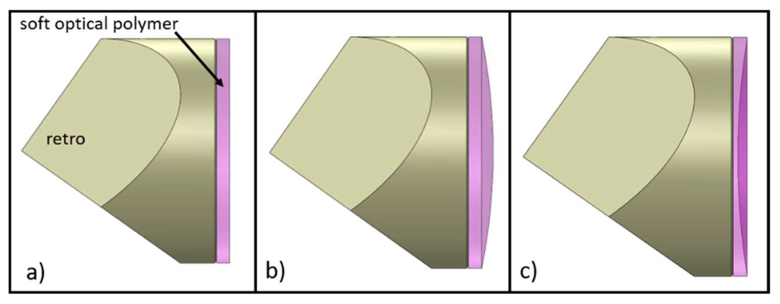
For the elastomeric optical polymer option, the elastic polymer is molded to a desired initial shape and the change on the polymer surface can be affected by means of applying a pressure/compression to the polymer. An elastomeric optical polymer is a polymer that has high transmission at the user-desired operational wavelength and has elastic properties which allow the solid substrate to be deformed. A second alternative to deform the polymer can be achieved by the use of dielectric elastomer actuation in which a voltage is applied to a pliable electrode and the polymer is deformed, creating the change on its surface.
Figure 1 shows the configuration of the elastomer optical polymer, as well as three operational states of the adaptive retroreflector.
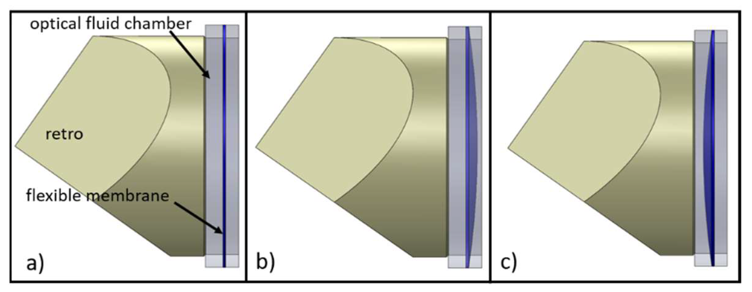
For a fluidic adaptive/tunable option, an elastomeric membrane encapsulates an optical fluid which is mounted on the front of a hollow or solid retroreflector. The elastomeric membrane needs to have similar optical and mechanical properties to those described above for the solid option. The optical fluid, needs to be optically and chemically compatible with the membrane and needs to have high transmission at the operational wavelength. Polydimethylsiloxane is a common polymer that can be used for the membrane as well as for the elastomeric solid option. For the optical fluids, there are numerous oils, polymers and resins that have been studied (for example, water, glycerol, etc.) [
3]. The actuation of this system can be achieved by compressing/decompressing the flexible membrane, which creates a change on its surface. This occurs by moving a cylinder along the optical axis of the system, thus compressing the circumference of the flexible membrane. Besides the mechanical action, magnetic actuation or use of a compliant electrode (dielectric elastomer) can achieve actuation of the membrane. There are other actuation techniques that are situatable and could be implemented as well, such as those used by commercially available fluidic lenses, for example, Varioptics, Optotune and Holochip [
6,
7,
8,
9,
10,
11,
12].
Figure 2, shows a conceptual sketch of the adaptive retroreflector based on the flexible membrane/fluidic concept.
The latter configuration was selected for this paper. The device changes the divergence of the returned beam but can also work as a regular passive retroreflector if the system requires.
3. Fabrication, Characterization and Results
Here, we present the optical design of the AR as fabricated and in the configuration we used for testing. We describe the optical setups used for testing and comparing the device to a passive retroreflector. Data for the repeatability and arbitrary radius of curvature measurements was acquired using a Zygo Verifire HD optical interferometer. Furthermore, we show images taken comparing a passive retroreflector in comparison with AR, both actuated and flat.
3.1. AR Optical Design
We used OpticStudio nonsequential tools to model the corner cube retroreflector and adaptive components and, for visualization purposes, a beam splitter cube was added, as shown in
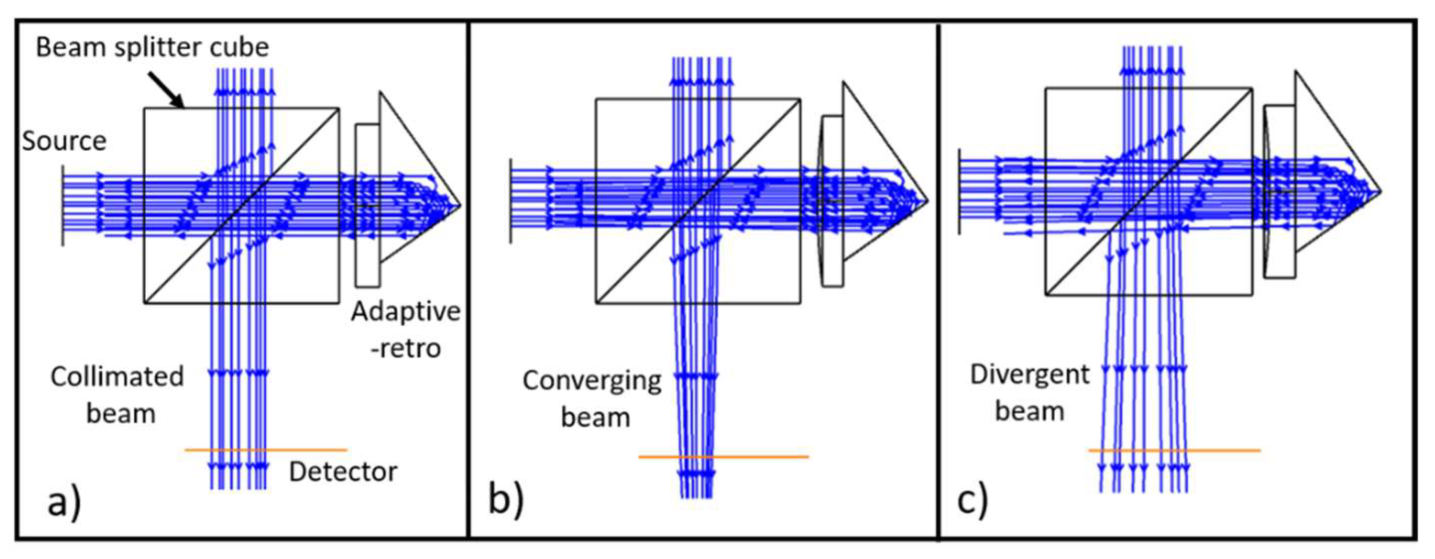
Figure 3. This was also the configuration chosen for the test. Note that we did not model the thickness of the membrane, since the effects of the membrane are negligible in OpticStudio for this type of application. The model was performed using the volume of the fluid, the fluid acting as a lens which changes its radius of curvature and center thickness. The figure shows a collimated beam, incident on a beam splitter cube which reflects part of the incident light and transmits a portion, which then impinges on the adaptive retroreflector. Light is reflected back from the retroreflector and reflected again from the beam splitter cube and incident on the detector. In field operations, the beam splitter can be used to monitor the incoming beam and direct the adaptive retroreflector in order to control the divergence. It can also be used without the beam splitter cube, such that the beam can be monitored at the receiver side and the system optimized in a power-in-the-bucket (PIB) configuration using well-known algorithms (e.g., stochastic parallel-gradient-descent) [
13,
14]; the AR is then instructed by this information.
3.2. Fabrication of the AR
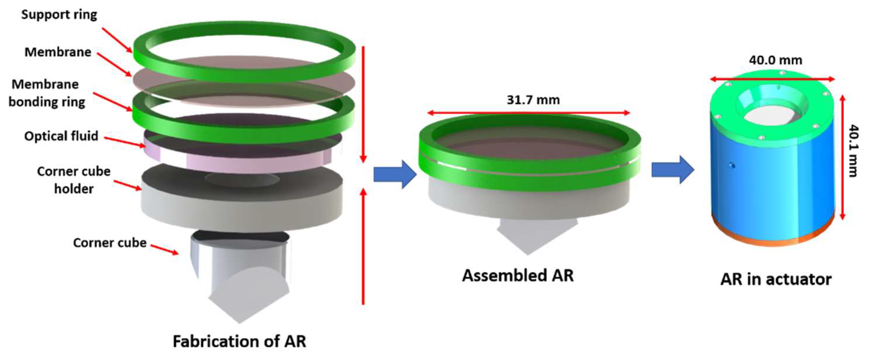
For this particular design we used a 12.7 mm corner cube retroreflector from Thorlabs, polydimethysiloxane (PDMS) as the membrane, glass support structures for the PDMS, and an optical fluid with an index of refraction of 1.45 and an Abbe number of 45.0 (at λ = 589 nm). The first step consisted in making the PDMS membrane which was then bonded to the glass support structure. The fluid was added to the membrane/glass structure and the corner cube was bonded to it. The last step was to mount the AR into the actuator and start the testing—the assembly steps are shown in
Figure 4. An important note: for this proof of concept, we did not follow the special fabrication procedures that we normally utilize to reduce the surface wavefront error which involve the reduction of coma induced by gravity and astigmatism resulting from the materials and fabrication procedures.
Figure 4 shows the top-level schematic of the assembly procedure, as well as pictures of the assembled AR (in its actuator). The actuator was custom-made for our adaptive lenses, and we were able to modify one to accommodate the AR. The actuator consists of a modified motor in a custom housing, with a maximum clear aperture of 19.5 mm, optical encoder with a resolution of ~50 nm, speed of ~2.5 mm/s, peak power consumption ~15 W, idle power consumption of ~1–500 µW and temperature monitoring of 0.01 °C. The electronics can control two actuators at the same time and can run off three CR-123 batteries (two batteries for a single actuator) with an average number of actuations of about 6000 per set of batteries.
3.3. Laboratory Optical Setup
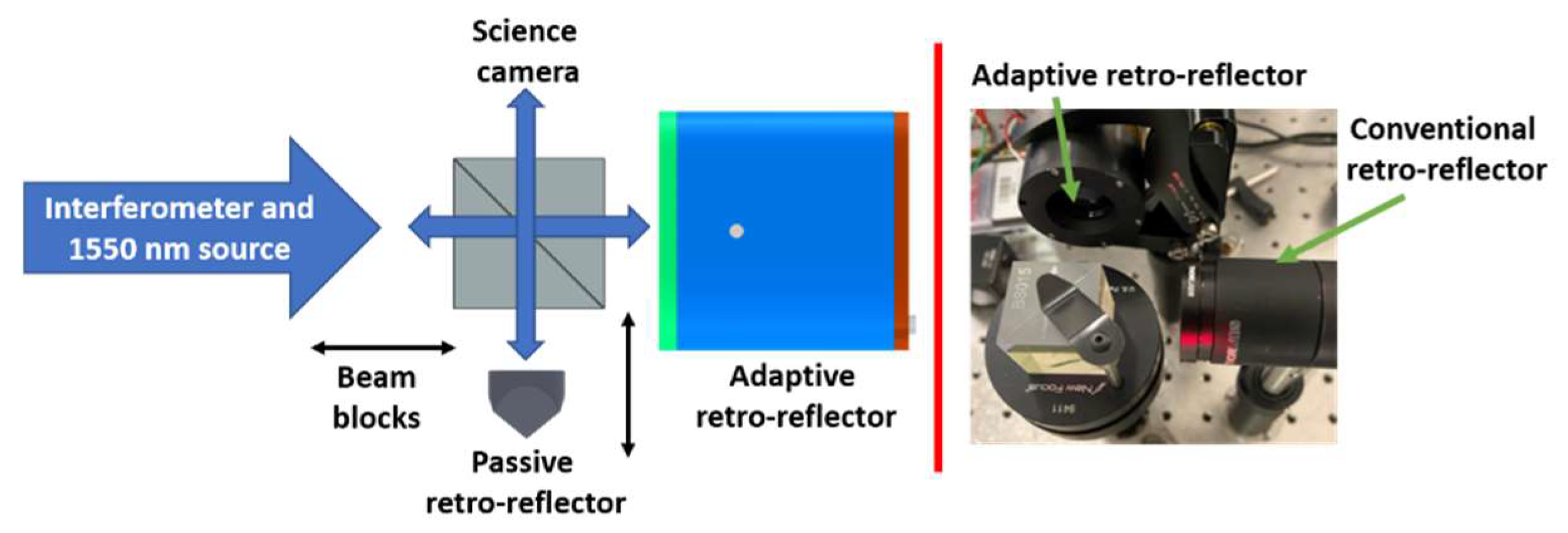
The AR was tested in various ways. Firstly, in the same way that we measured the radius of curvature (ROC) of lenses using a Zygo interferometer—for this device we measured two ROCs as a test, a positive (convex surface) with a ROC of 234 mm and a negative (concave surface) of −185 mm. The second setup was to compare the performance and proof of concept of the AR in comparison with a passive retroreflector, as shown in
Figure 5. We used the HeNe 633 nm source of the Zygo interferometer and a 1550 nm was co-aligned for further testing. Data from the 1550 nm was not included but performance of the active surface component at this wavelength has been demonstrated in a previous report [
5]. We were able to use the beam collimated or with the addition of a known divergence that could be removed with the AR and compared with the passive retroreflector. The setup with the beam splitter cube allowed us to look at the return beam with the interferometer and, on the other arm, to look at the output with a camera, photodetector or power meter, while we were able to use beam blocks to look at each retroreflector individually or additionally, enabling viewing of the interference fringes formed by the two. This facilitated alignment, but also monitoring of the difference when the AR is actuated. This same setup was also used to perform first order measurements of the repeatability of the AR by actuating the AR from a flat state to a convex or concave state and back to a flat state, while measuring the surface form with the interferometer. An important note: temperature was monitored in the room, but temperature compensation of the AR was not used—the room environment was stable and thus compensation was not required.
3.4. Results/Discussion
3.4.1. ROC and Surface Measurements
The first test consisted of measurements of the ROC, positive and negative, in order to evaluate the performance of the device.
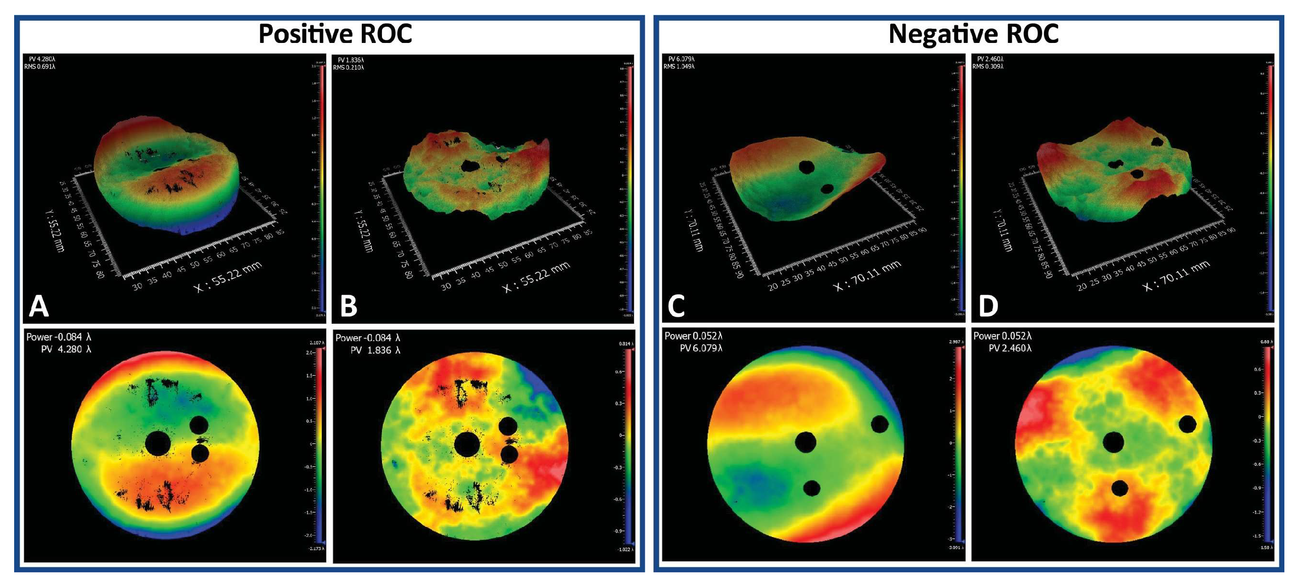
Figure 6 shows a set of measurements, including a (left) measurement for a positive ROC of 255 mm and a (right) measurement for a negative ROC of 184 mm. The top row shows the 3D surface profile, and the bottom row indicates the 2D profile. The black circles in the figure are software masks used to remove unnecessary back reflections created by dust particles in the reference sphere. Within the respective figures, the left column (A or C) is the raw measurement and the right side (B or D) is with the dominant aberrations removed. As mentioned before, fabrication was not optimized for the surface figure, but what can be seen is the typical dominant aberration of coma and astigmatism, which are characteristic for this type of fluidic structures. Coma is due to gravity and astigmatism is due to fabrication or assembly procedures. For the positive ROC case demonstrated below, coma is the dominant aberration. On the negative ROC, there is a combination of coma and astigmatism, because measurements were taken close to the negative resting ROC (fabricated ROC) of the membrane for the fabricated AR device. The fabricated aberrations were more noticeable closer to the resting ROC because, for this type of actuation mechanism, this is the point of contact where boundary conditions are established between the membrane and actuation surface for the clear aperture. At this point, the amplitude of any existing aberrations can be enhanced. Another aberration that can be noticed is trefoil on both ROCs—this was purely due to the assembly in the actuator. We developed procedures for fabrication and assembly that reduce the dominant aberrations which are implemented when building adaptive polymer lenses, with the caveat that we can minimize coma based on the application, but do not completely eliminate it. The procedure to eliminate coma during fabrication is extremely complex, costly and time consuming if performed at the active surface. There are other ways to minimize it, including using a corrective element along the optical path of the system or close to the active surface, and this is a typical configuration used in commercial adaptive/tunable lenses [
11].
Using the data from
Figure 6, a Zernike fit was performed using the Mx software tools from the interferometer and coefficients of the fit for both the positive and negative ROCs are shown in
Table 1.
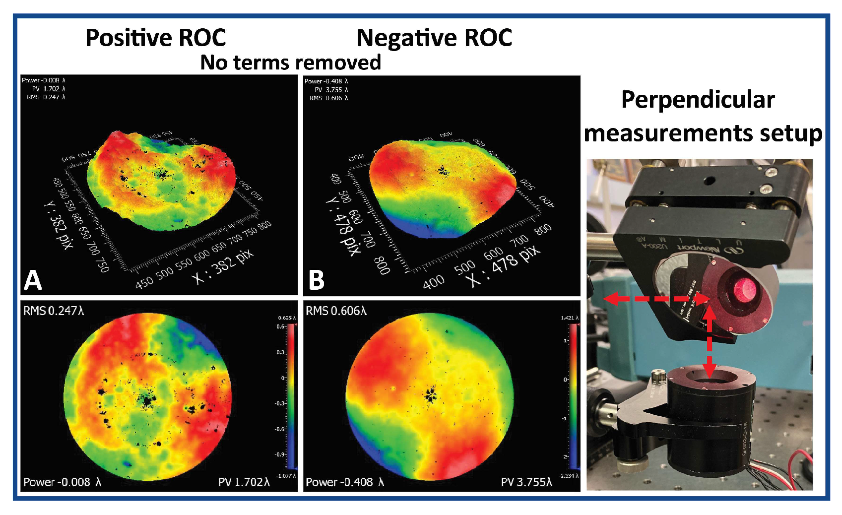
Figure 7, shows data taken for the AR at the same ROCs mentioned above but in a perpendicular configuration in order to eliminate the effects of coma due to gravity. Note, that for the data no terms have been removed. Astigmatism and trefoil were noticeable but the large magnitude due to coma was absent.
The same procedure was performed on the results from
Figure 7 and
Table 2 shows the Zernike fit coefficients for the perpendicular measurements.
3.4.2. Repeatability Measurements
Repeatability measurements were taken using the setup in
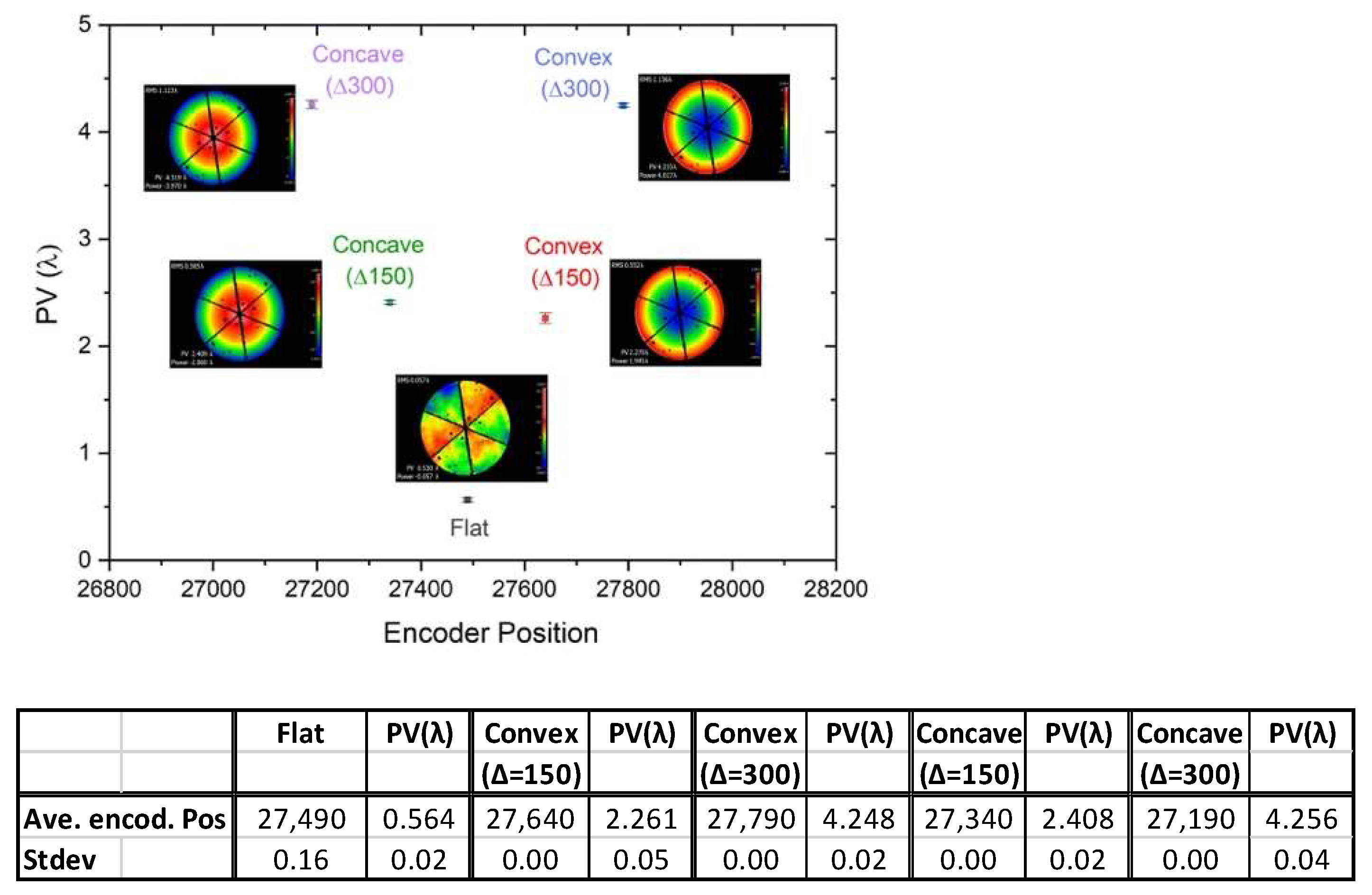
Figure 5. The data collection consisted in changing the actuation state by a known encoder count from a flat state to a convex/concave state, while recording the encoder position as well as the data from the inferferometer. The encoder data is in the form of a set of three numbers: the set position by user (state of the lens), the temperature compensate position (once thermal compensation is activated) and the measured position. This last position, or the difference from the set position, was recorded. Readings from the interferometer PV(λ) (peak to valley) and power(λ) were recorded as well. Data was taken for a delta for encoder counts of 150 and 300 from flat, on both positive (convex or higher encoder counts), and negative (concave or lower encoder counts) direction.
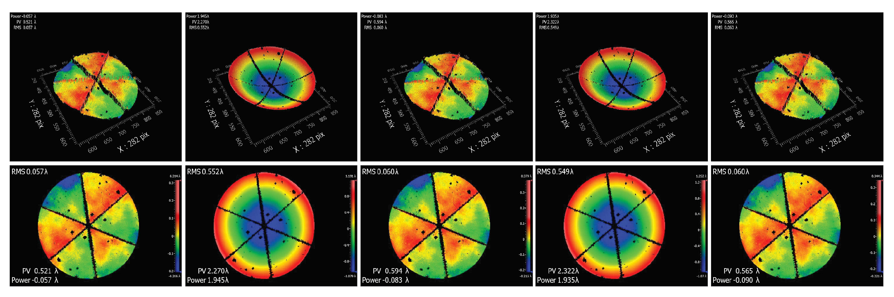
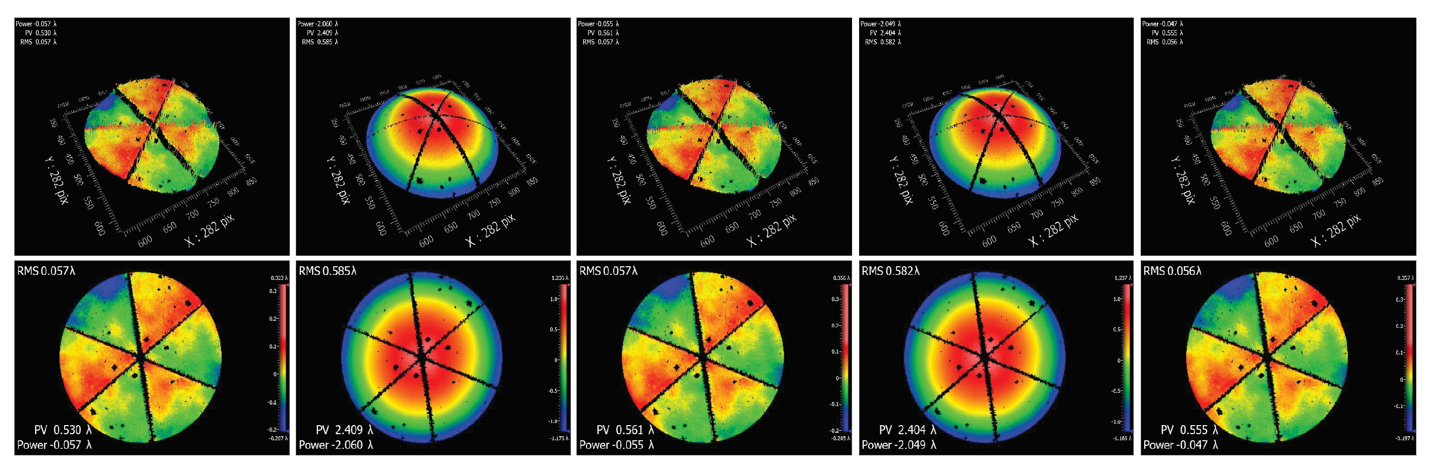
Figure 8 shows a sequence of consecutive measurements from flat to positive and
Figure 9 shows measurements from flat to negative for a delta of 150 encoder counts. Note, the hexagonal pattern was a result of the facets of the corner cube. This was noticeable in this configuration based on the testing setup with the interferometer using a transmission flat. For the ROCs the measurements differed, since we were using a reference sphere and the spherical wavefront matched the deformed membrane, not the retroreflector.
In
Figure 10, data is presented in graphical (with error bars based on the standard deviation), and tabular, form for the sequences, with 20 data points for delta 150 and 10 points for delta 300, and all cases starting from the same initial flat position. The average and standard deviation for the encoder position and peak-to-valley for the cases are shown in the table.
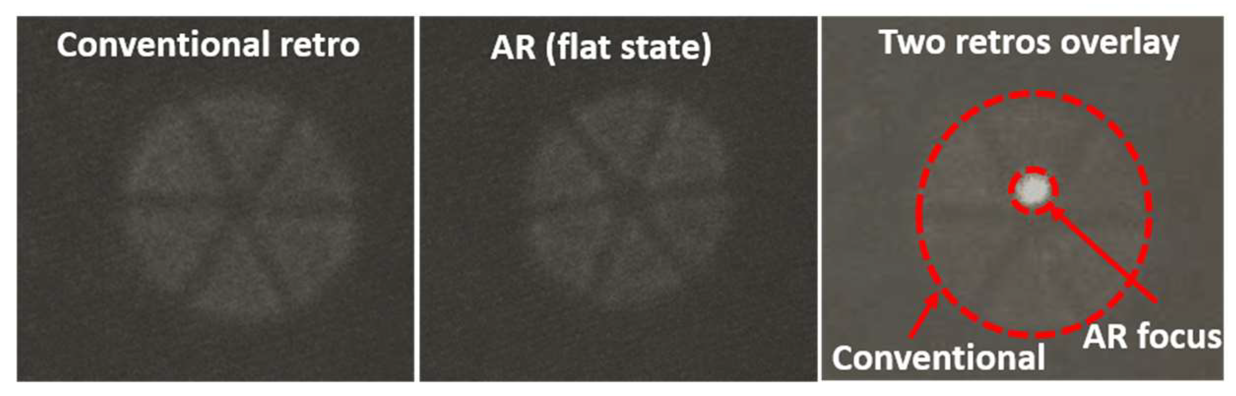
Figure 11 shows a comparison of the AR with a passive retroreflector. A screen was placed at a distance of approximately 1500 mm and the response from a collimated beam recorded and the AR was actuated in order to focus the beam on the screen.
4. Conclusions
We have presented the concept of an adaptive retroreflector. This concept was developed during a data campaign to study the atmospheric turbulence in a dynamic link, with the end goal of an optical anemometer for UAV applications in which the propagation distance is changing rapidly. The concept of the AR was then designed, fabricated and tested in a laboratory environment as a proof of concept. This particular device can operate from the VIS to the SWIR and preliminary parameters of its performance were studied. The next step will consist of fabricating a device following the tighter tolerance procedures developed previously for adaptive lenses. A follow-up report will consist of performing a calibration in a laboratory environment, including thermal compensation and quantification of losses added by absorption and/or scattering due to the membrane/fluid combination in comparison with a conventional retroreflector. The latter case will be studied in more detail in a field experiment where we can compare the losses due to the addition of the membrane/fluid combination with the losses of a conventional retroreflector (e.g., due to diffraction, or divergence introduced by atmospheric turbulence) at a propagation path. A power-in-the-bucket configuration will be used to compare the divergence control of the adaptive retroreflector and a conventional one. While the overall losses depend on configuration and materials, our experience with fluidic lenses has shown that the transmission losses are negligible compared to effects induced by turbulence.
5. Patents
A provisional patent application has been submitted, U.S. Patent Application Serial No. 62/695,310.
Author Contributions
Conceptualization, F.S. and C.O.F.; methodology, F.S., C.O.F., B.E.B. and S.R.R.; formal analysis, F.S., S.N.Q. and S.R.R.; writing—original draft preparation, F.S., C.O.F., S.R.R.; writing—review and editing, S.R.R., S.N.Q. and B.E.B.; funding acquisition, F.S. All authors have read and agreed to the published version of the manuscript.
Funding
This research received no external funding.
Institutional Review Board Statement
Not applicable.
Informed Consent Statement
Not applicable.
Data Availability Statement
Data is contained within the article.
Conflicts of Interest
The authors declare no conflict of interest.
References
- Font, C.; Apker, T.; Santiago, F. Laser Anemometer for Autonomous Systems Operations. In AIAA Infotech@ Aerospace; AIAA SciTech: San Diego, CA, USA, 2016; p. 1230. [Google Scholar] [CrossRef]
- Font, C.; Santiago, F.; Apker, T. Atmospheric Turbulence Measurements in Dynamical Links. In Propagation Through and Characterization of Atmospheric and Oceanic Phenomena, OSA Technical Digest (Online), 3rd ed.; Paper M2A.3.; Optical Society of America: Washington, DC, USA, 2016; pp. 154–196. [Google Scholar]
- Santiago, F.; Bagwell, B.; Martinez, T.; Restaino, S.; Krishna, S. Large aperture adaptive doublet polymer lens for imaging applications. J. Opt. Soc. Am. A 2014, 31, 1842–1846. [Google Scholar] [CrossRef]
- Santiago, F.; Font, C.; Restaino, S. Adaptive Polymer Lenses at NRL. In Applied Industrial Optics 2019, OSA Technical Digest; Paper T2A.2.; Optical Society of America: Washington, DC, USA, 2019. [Google Scholar]
- Santiago, F.; Bagwell, B.E.; Pinon, V., III; Krishna, S. Adaptive polymer lens for rapid zoom shortwave infrared imaging applications. Opt. Eng. 2014, 53, 125101. [Google Scholar] [CrossRef]
- Berge, B.; Peseux, J. Variable focal lens controlled by an external voltage: An application of electrowetting. Eur. Phys. J. E 2000, 3, 159–163. [Google Scholar] [CrossRef]
- Berge, B. Electrocapillarite et mouillage de films isolants par l’eau. C.R. Acad. Sci. Ser. II Mec. Phys. Chim. Sci. Terre Univ. 1993, 317, 157. [Google Scholar]
- Mugele, F.; Baret, J. Electrowetting: From basics to applications. J. Phys. Condens. Matter IOP Publ. 2005, 17, R705–R774. [Google Scholar] [CrossRef]
- Heikenfeld, J.; Smith, N.; Dhindsa, M.; Zhou, K.; Kilaru, M.; Hou, L.; Zhang, J.; Kreit, E.; Raj, B. Recent Progress in Arrayed Electrowetting Optics. Opt. Photonics News 2009, 20, 20–26. [Google Scholar] [CrossRef]
- Yiu, J.; Batchko, R.; Robinson, S.; Szilagyi, A. A fluidic lens with reduced optical aberration. In Intelligent Robots and Computer Vision XXIX: Algorithms and Techniques; Proc. SPIE 8301; SPIE: Burlingame, CA, USA, 2012; p. 830117. [Google Scholar]
- Blum, M.; Büeler, M.; Grätzel, C.; Giger, J.; Aschwanden, M. Optotune focus tunable lenses and laser speckle reduction based on electroactive polymers. In MOEMS and Miniaturized Systems XI; Proc. SPIE 8252; SPIE: San Francisco, CA, USA, 2012; p. 825207. [Google Scholar]
- Vorontsov, M.A.; Sivokon, V.P. Stochastic parallel-gradient-descent technique for high-resolution wave-front phase-distortion correction. J. Opt. Soc. Am. A 1998, 15, 2745–2758. [Google Scholar] [CrossRef]
- Font, C.O.; Gilbreath, G.C.; Bajramaj, B.; Kim, D.S.; Santiago, F.; Martinez, T.; Restaino, S.R. Characterization and training of a 19-element piezoelectric deformable mirror for lensing. J. Opt. Fiber. Commun. Res. 2010, 7, 1–9. [Google Scholar] [CrossRef]
- Ma, S.; Yang, P.; Lai, B.; Su, C.; Zhao, W.; Yang, K.; Jin, R.; Cheng, T.; Xu, B. Adaptive Gradient Estimation Stochastic Parallel Gradient Descent Algorithm for Laser Beam Cleanup. Photonics 2021, 8, 165. [Google Scholar] [CrossRef]
Figure 1.
Schematic of an adaptive retroreflector using a solid elastomeric polymer: (a) flat (b) convex and (c) concave.
Figure 1.
Schematic of an adaptive retroreflector using a solid elastomeric polymer: (a) flat (b) convex and (c) concave.
Figure 2.
Schematic of an adaptive retroreflector using an optical liquid/fluidic: (a) flat (b) convex and (c) concave.
Figure 2.
Schematic of an adaptive retroreflector using an optical liquid/fluidic: (a) flat (b) convex and (c) concave.
Figure 3.
Optical design setup used for testing including the collimated source incident on the beam splitter cube with the outputs: (a) a collimated beam, (b) a converging beam, and (c) a divergent beam.
Figure 3.
Optical design setup used for testing including the collimated source incident on the beam splitter cube with the outputs: (a) a collimated beam, (b) a converging beam, and (c) a divergent beam.
Figure 4.
Schematic representation of the fabrication and assembly process of the AR.
Figure 4.
Schematic representation of the fabrication and assembly process of the AR.
Figure 5.
(Left) Layout of the optical testing setup. (Right) Picture of optical devices used for measurements.
Figure 5.
(Left) Layout of the optical testing setup. (Right) Picture of optical devices used for measurements.
Figure 6.
(Left) Positive ROC measurement (A,B columns) 2D and 3D profiles with dominant aberration removed, in this instance being coma (B column). (Right) Negative ROC measurement (C,D columns) 2D and 3D profiles with dominant aberration removed, in this instance, coma and astigmatism (D column).
Figure 6.
(Left) Positive ROC measurement (A,B columns) 2D and 3D profiles with dominant aberration removed, in this instance being coma (B column). (Right) Negative ROC measurement (C,D columns) 2D and 3D profiles with dominant aberration removed, in this instance, coma and astigmatism (D column).
Figure 7.
(A) Positive and (B) negative ROC, 2D and 3D surface representation for the perpendicular setup. Right side shows a picture of the setup.
Figure 7.
(A) Positive and (B) negative ROC, 2D and 3D surface representation for the perpendicular setup. Right side shows a picture of the setup.
Figure 8.
The AR was actuated from the flat state to a compressed state (or convex surface) and back to flat. For each case the top row is the 3D surface and the bottom row the 2D surface.
Figure 8.
The AR was actuated from the flat state to a compressed state (or convex surface) and back to flat. For each case the top row is the 3D surface and the bottom row the 2D surface.
Figure 9.
The AR was actuated from the flat state to a less compressed state (or concave surface) and back to flat. For each case the top row is the 3D surface and the bottom row the 2D surface.
Figure 9.
The AR was actuated from the flat state to a less compressed state (or concave surface) and back to flat. For each case the top row is the 3D surface and the bottom row the 2D surface.
Figure 10.
Graphical and tabular representation of the actuation sequence for the cases described above. Delta values refer to the change in encoder position from the flat state.
Figure 10.
Graphical and tabular representation of the actuation sequence for the cases described above. Delta values refer to the change in encoder position from the flat state.
Figure 11.
Images taken in the laboratory at a known distance from the retroreflector are shown (left) conventional retroreflector, (middle) AR in the flat state, and (right) both retroreflectors overlapping in the screen with the AR actuated to focus the beam at that particular distance.
Figure 11.
Images taken in the laboratory at a known distance from the retroreflector are shown (left) conventional retroreflector, (middle) AR in the flat state, and (right) both retroreflectors overlapping in the screen with the AR actuated to focus the beam at that particular distance.
Table 1.
Results from the Zernike fit coefficients obtained from the data in
Figure 6, for positive ROC (top) and negative ROC (bottom).
Table 1.
Results from the Zernike fit coefficients obtained from the data in
Figure 6, for positive ROC (top) and negative ROC (bottom).
| ROC = 225 mm |
| Zernike Fit |
| Coeff | Value (λ) | n | m | Representation |
| ZFR 0 | 0.000 | 0 | 0 | 1 |
| ZFR 1 | 0.000 | 1 | 1 | ρcos(θ) |
| ZFR 2 | 0.000 | 1 | −1 | ρsin(θ) |
| ZFR 3 | 0.018 | 2 | 0 | −1 + 2ρ2 |
| ZFR 4 | −0.085 | 2 | 2 | ρ2cos(2θ) |
| ZFR 5 | −0.407 | 2 | −2 | ρ2sin(2θ) |
| ZFR 6 | −0.122 | 3 | 1 | (−2ρ + 3ρ3)cos(θ) |
| ZFR 7 | 2.191 | 3 | −1 | (−2ρ + 3ρ3)sin(θ) |
| ZFR 8 | −0.047 | 4 | 0 | 1 − 6ρ2 + 6ρ4 |
| ROC = −184 mm |
| Zernike Fit |
| Coeff | Value (λ) | n | m | Representation |
| ZFR 0 | 0.000 | 0 | 0 | 1 |
| ZFR 1 | 0.000 | 1 | 1 | ρcos(θ) |
| ZFR 2 | 0.000 | 1 | −1 | ρsin(θ) |
| ZFR 3 | −0.049 | 2 | 0 | −1 + 2ρ2 |
| ZFR 4 | −0.211 | 2 | 2 | ρ2cos(2θ) |
| ZFR 5 | −1.823 | 2 | −2 | ρ2sin(2θ) |
| ZFR 6 | −0.108 | 3 | 1 | (−2ρ + 3ρ3)cos(θ) |
| ZFR 7 | −2.115 | 3 | −1 | (−2ρ + 3ρ3)sin(θ) |
| ZFR 8 | −0.372 | 4 | 0 | 1 − 6ρ2 + 6ρ4 |
Table 2.
Results from the Zernike fit coefficients obtained from the data in
Figure 7, for positive ROC (top) and negative ROC (bottom).
Table 2.
Results from the Zernike fit coefficients obtained from the data in
Figure 7, for positive ROC (top) and negative ROC (bottom).
| ROC = 225 mm Perpendicular |
| Zernike Fit |
| Coeff | Value (λ) | n | m | Representation |
| ZFR 0 | 0.000 | 0 | 0 | 1 |
| ZFR 1 | 0.000 | 1 | 1 | ρcos(θ) |
| ZFR 2 | 0.000 | 1 | −1 | ρsin(θ) |
| ZFR 3 | 0.038 | 2 | 0 | −1 + 2ρ2 |
| ZFR 4 | 0.137 | 2 | 2 | ρ2cos(2θ) |
| ZFR 5 | −0.390 | 2 | −2 | ρ2sin(2θ) |
| ZFR 6 | 0.065 | 3 | 1 | (−2ρ + 3ρ3)cos(θ) |
| ZFR 7 | −0.071 | 3 | −1 | (−2ρ + 3ρ3)sin(θ) |
| ZFR 8 | −0.099 | 4 | 0 | 1 − 6ρ2 + 6ρ4 |
| ROC = −184 mm Perpendicular |
| Zernike Fit |
| Coeff | Value (λ) | n | m | Representation |
| ZFR 0 | 0.000 | 0 | 0 | 1 |
| ZFR 1 | 0.000 | 1 | 1 | ρcos(θ) |
| ZFR 2 | 0.000 | 1 | −1 | ρsin(θ) |
| ZFR 3 | −0.202 | 2 | 0 | −1 + 2ρ2 |
| ZFR 4 | −0.052 | 2 | 2 | ρ2cos(2θ) |
| ZFR 5 | −1.248 | 2 | −2 | ρ2sin(2θ) |
| ZFR 6 | 0.126 | 3 | 1 | (−2ρ + 3ρ3)cos(θ) |
| ZFR 7 | −0.112 | 3 | −1 | (−2ρ + 3ρ3)sin(θ) |
| ZFR 8 | −0.224 | 4 | 0 | 1 − 6ρ2 + 6ρ4 |
| Publisher’s Note: MDPI stays neutral with regard to jurisdictional claims in published maps and institutional affiliations. |
© 2022 by the authors. Licensee MDPI, Basel, Switzerland. This article is an open access article distributed under the terms and conditions of the Creative Commons Attribution (CC BY) license (https://creativecommons.org/licenses/by/4.0/).

 ,
, 


