Identification of Model Particle Mixtures Using Machine-Learning-Assisted Laser Diffraction

Abstract

We put forward and demonstrate with model particles a smart laser-diffraction analysis technique aimed at particle mixture identification. We retrieve information about the size, shape, and ratio concentration of two-component heterogeneous model particle mixtures with an accuracy above 92%. We verify the method by detecting arrays of randomly located model particles with different shapes generated with a Digital Micromirror Device (DMD). In contrast to commonly-used laser diffraction schemes—In which a large number of detectors are needed—Our machine-learning-assisted protocol makes use of a single far-field diffraction pattern contained within a small angle (∼0.26°) around the light propagation axis. Therefore, it does not need to analyze particles of the array individually to obtain relevant information about the ensemble, it retrieves all information from the diffraction pattern generated by the whole array of particles, which simplifies considerably its implementation in comparison with alternative schemes. The method does not make use of any physical model of scattering to help in the particle characterization, which usually adds computational complexity to the identification process. Because of its reliability and ease of implementation, this work paves the way towards the development of novel smart identification technologies for sample classification and particle contamination monitoring in industrial manufacturing processes.

1. Introduction

Particle characterization techniques have long played a fundamental role in many different branches of science and technology. In biology, they assist in schemes for the detection of bacteria [1] and viruses [2]. They are important in the pharmaceutical [3,4], food processing [5,6], and the semiconductor industries [7]. Particularly important are applications aimed at environmental monitoring and protection [8,9]. Some potential applications include the detection of microplastics in marine waters [10], and the characterization of airborne particles, given that their size is strongly correlated with pulmonary toxicity [11,12] leading to respiratory illnesses.

Remarkably, more than 75% of all materials processed in the industry are in particulate form. These particles may be contained in substances in any of the three known phases (solid, liquid, or gaseous) and can be divided into three broad groups: natural, industrially processed from natural products, and completely synthetic particles [13]. In general, one can identify two important reasons for industries routinely employing particle characterization [14]: better understanding of products and processes, and better control of product quality. While the former allows for the optimization of the manufacturing processes, the latter can translate into a potentially important economic benefit.

During the past two decades, several light scattering technologies used for particle characterization have matured and even become a key part of industrial production lines [15]. These techniques may be classified into three main categories: static light scattering (SLS), dynamic light scattering (DLS), and scattering tracking analysis (STA). In the first class, the measured scattering signal results from the light-particle interaction at various spatial locations, whereas in the second and third, the recorded signal results from the monitoring of light-particle interaction as a function of time.

Different techniques aim, or are better suited, for particles in different size classes. Particle dimension ranges from very small, such as viruses (20–100 nm) [16], to larger ensembles such as bacteria colonies of 1–2 mm dimension, with a number of possible shapes [1]. For instance, while dynamic light scattering techniques can resolve particles deep in the submicron region [17], static methods work best in the range of hundreds of $\mathsf{\mu }$m to mm [18,19]. Here we aim at this regime of size particles, with the smaller particles considered being tens of microns in size.

Static light scattering, also known as laser diffraction (LD) analysis has become the most widely used technique for extracting information about the particle size distribution of an unknown sample [20]. This technique is based both on Mie light scattering theory, and on far-field Fraunhofer diffraction. In LD analysis, the light intensity vs scattering angle is related to the dimensions of the particles participating in the scattering process, with other variables, such as wavelength, kept constant. Thus, information about particle size is extracted from the angular intensity variation of laser light scattered from a given sample: larger particles scatter light at smaller angles, while smaller particles scatter at wider angles [14]. It is worth pointing out that while for Fraunhofer diffraction the particle size analysis is somewhat straightforward, the Mie scattering approach requires knowledge of the real and imaginary parts of the sample’s refractive index [13].

Commercial LD instruments have been used extensively in the industry due to their high precision and reliability. Important drawbacks include their limited portability and their inability to fully discern among different particle shapes. In particular, given that LD is based on the precise detection at different scattering angles, typical instruments require in the region of 16 to 32 detectors positioned at different angles with respect to the main optical axis (see, for instance, Figure 4 of Ref. [15]). Unfortunately, increasing the number of detectors does not necessarily lead to a better resolution [18] and thus, finding the optimum number and location of detectors for a particular application becomes a crucial task. Most LD schemes are based upon the assumption that particles, although different in size, are always spherical; this poses a problem if the goal is to identify samples containing particles with different shapes [21,22].

Although it is well known that particle shape influences the properties and behavior of substances, for example affecting material strength and deformation mechanisms [23] as well as the compaction/flux of powders [24], it remains challenging to determine it experimentally. Some studies have used LD for the development of sensors to obtain particle shape information for online process control and monitoring, however, these have only achieved limited success [25,26]. Many different measures have been suggested for the characterization of particle shape, involving roundness and angularity (sharpness) [27,28]. More rigorously, extensions of the Mie theory for arbitrarily-shaped particles can be approached numerically; however, applying such numerical solutions to mixtures of many particles would be computationally very costly [29,30].

Neural network (NN) algorithms have been applied for particle characterization allowing for the estimation of relevant parameters such as particle size and concentration. In addition, they have also been shown to outperform ill-conditioned inverse scattering problems in Mie theory by reducing significantly the required computational time [31]. In this sense, machine learning (ML) techniques are known to be powerful for pattern recognition in large data sets, providing reliable parameter estimation. The standard procedure is to train NNs with either experimental or synthetic data spanning the parameter range of interest, and subsequently estimate the desired parameters by using measurements as input to the trained NN [32]. The key point is that NNs make use of their self-learning capabilities to enhance the performance of optical systems in terms of reliability and resolution without the need to increase their complexity. ML techniques have been applied for particle shape characterization by recognizing the morphology of particle aggregation, ref. [33] or by defining the boundaries of each particle from direct imaging measurements [34]. Interestingly, neural networks have been shown to significantly improve the detection of spatial features in out-of-the-lab technologies such as mobile-phone-based microscopes [35]. These features combined undoubtedly facilitate the deployment of machine-learning-assisted methods in industrial settings.

In this work, we provide the first steps towards “smart” laser diffraction analysis of heterogeneous mixtures [36]. This technique makes use of a trained artificial NN to identify spatial features of heterogeneous mixtures of microscopic objects. Our analysis relies on monitoring the far-field diffraction pattern produced by laser light impinging on two-dimensional arrays of model particles which, for the sake of simplicity and generality, are simulated with the help of a Digital Micromirror Device (DMD). We would like to point out that, although these model particles are not real three-dimensional objects, they exhibit certain advantages [37,38]. In particular, given their two-dimensional nature, they reasonably fulfill the theoretical pre-assumptions for Fraunhofer diffraction, and by excluding other possible effects derived from real three-dimensional particles help focus our attention on the advantages of using smart technologies, i.e., those based on pre-programmed rules or patterns learned during a training stage, for laser diffraction analysis.

The technique hereby proposed, in which relevant sample information is reliably extracted from a single and static far-field diffraction pattern, offers two main advantages over typical LD devices. Firstly, it allows for efficient particle identification by detecting the signal within a small angle (∼0.26°) with respect to the light propagation axis, thus effectively reducing the number of detectors needed for its implementation, as is also the case in recent micro- and nano-particle identification proposals that make use of Machine Learning (ML) algorithms [31,39,40,41,42,43].

Secondly, our technique permits the identification of particle shapes in two-component heterogeneous mixtures resolving the shapes of the particles that make up the mixture, as opposed to currently available techniques in which only the particle size can be obtained [36,44]. In addition, this proposed technique allows for the determination of the predominance (or balance) between particle geometries. These features might be relevant for monitoring particle contamination in industrial manufacturing processes [45].

2. Experimental Methods

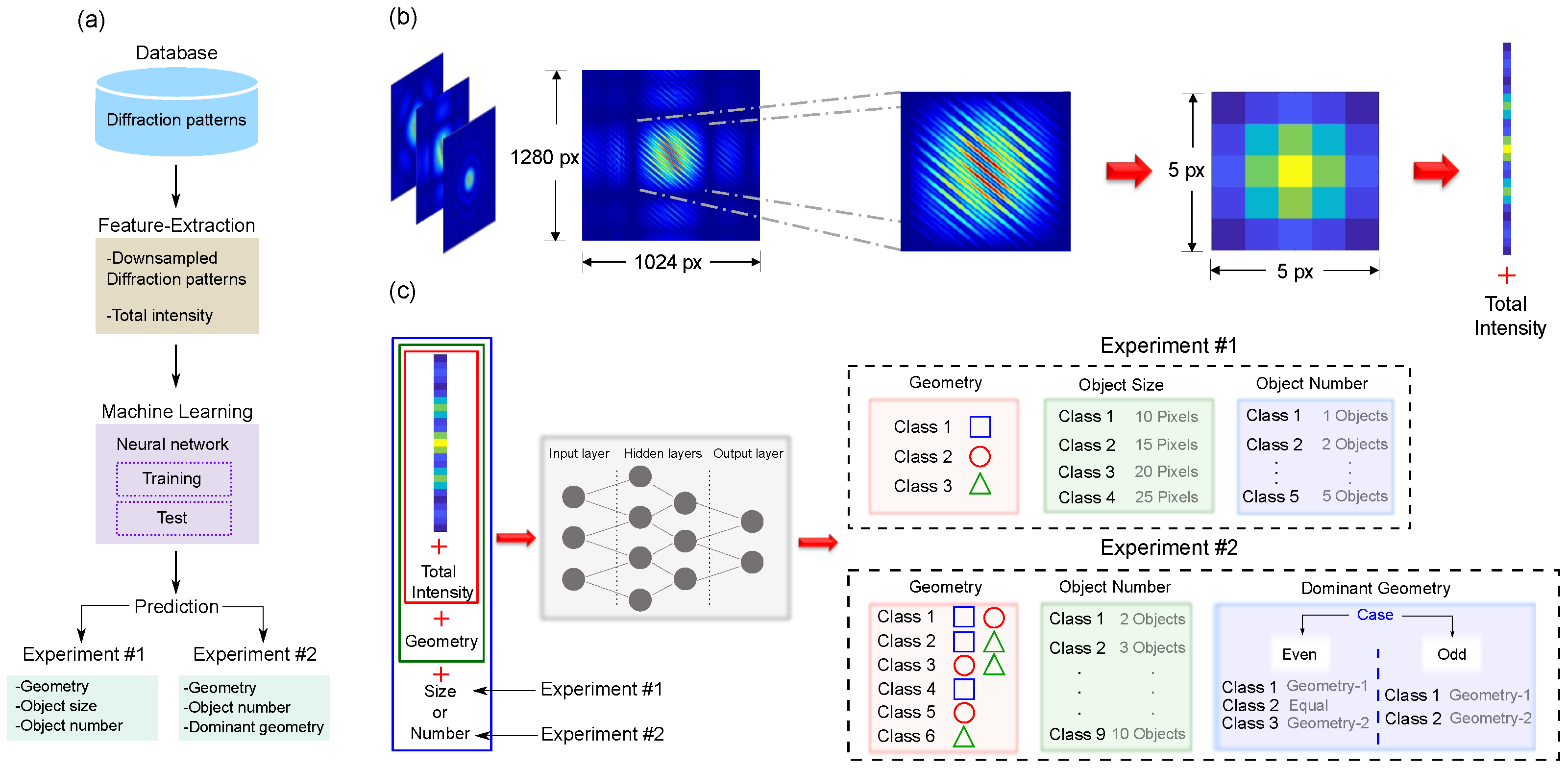
2.1. Setup and Data Acquisition

To generate a large set of different particle mixture configurations, we create objects of different geometries and sizes using a DMD consisting of a 6.57  mm × 3.69  mm chip containing a grid of square mirrors of $7.63\mathsf{\mu }$m per side. The mirrors can be selectively rotated ±12° in an “on” or “off” configuration such that when illuminated, the DMD reflects light selectively.

The DMD is illuminated with a 405 nm wavelength collimated beam of 2.46 mm diameter. The beam size is set to be smaller than the DMD window to avoid diffraction effects caused by the borders of the chip. Each object in the mixture corresponds to a contiguous array of mirrors in the “on” configuration that reflects a part of the beam. The objects are randomly positioned on the DMD plane assuring no overlap between particles. Due to the periodicity of the mirror grid, a mesh of diffraction order beams is produced. A single diffraction order is selected to be transmitted through a Fourier transform lens, and the diffraction pattern is collected with a CCD camera, as shown in Figure 1. Note that due to the dimensions of the beam, the model particle images, and the focal length of the Fourier lens L5 (200 mm), the DMD diffraction orders are naturally separated with propagation, so that no additional spatial filtering is required to isolate a single diffraction order. The collected diffraction patterns are stored as bitmaps, scaling the intensity values monitored with the CCD camera to 8-bits, associating the maximum intensity (saturated detector) to 255 gray-scale values.

We consider mixtures of microscopic particles. The aim is to retrieve information such as their size, geometry (shape), and concentration. To demonstrate in principle the effectiveness of the method, in this work we consider only three geometries, namely: squares, triangles, and circles. However, our results seem to indicate that one can consider two-dimensional arbitrarily shaped objects in more general scenarios, given that the different shapes to be identified produce a spatial far-field pattern which is sufficiently distinguishable. These mixtures are analyzed following the steps shown as a flowchart in Figure 2a.

To demonstrate that we can successfully retrieve the sought-after information about the microscopic objects, we carry out two different experiments. The first experiment (Experiment #1) aims at recognizing sets of microscopic objects that have the same shape but different characteristic lengths; in this case: 11, 15, 21, or 25 times the DMD mirror length (7.63 $\mathsf{\mu }$m). The total number of particles varies from one to five.

The second experiment (Experiment #2) considers mixtures containing two types (out of the three available geometries) of microscopic objects. In this experiment, the size of the particles is kept constant (15 micromirrors), while the total number of objects ranges from 2 to 10. All possible combinations $n_1+n_2=N$ are considered, where $n_1$ and $n_2$ are the number of sources belonging to geometries 1 and 2, respectively. The dataset for each experiment is created by randomly assigning the position of the objects, avoiding any overlap between them, and registering their corresponding far-field diffraction pattern. One hundred diffraction patterns were considered for each category. Given the total number of combinations of size, shape, and number of objects, Experiment #1 contains 6000 experimental diffraction patterns, while Experiment #2 includes 19,200 patterns.

Due to the quadratic scaling of the illuminated area with the increase of the particles’ characteristic length, the intensity of the diffraction pattern increases accordingly. Thus, in order to avoid saturation of the detector, and incomparable powers of the stored diffraction patterns, the power of the initial illumination beam was selected according to the total illuminated area; more precisely, the total number of pixels in the “on” configuration, which varied from 66 pixels (corresponding to a triangle of 11 pixels per side) up to an almost fifty times larger illuminated area of 3125 pixels (corresponding to five squares of 25 pixels per side).

Table 1. Beam power as a function of the illuminated area in the DMD.

Number of Pixels	Power [$\mathsf{\mu }$W]
≤500	200
501–1000	100
1001–1500	50
1501–3000	25
≥3001	15

summarizes the power of the illuminating beam for each case.

Because the illumination beam has a Gaussian profile, the power reflected by the DMD strongly depends on the distribution of the particles; the particles closer to the center of the beam will reflect more intense light than particles far from the center. Tailored illumination with uniform intensity profile such as top-hat beams would prevent this from happening, however, this requires alternative beam shaping equipment. To take these variations into account, we make sure that, in each case, the collected images had the same mean total power. To do so, the exposure time of each measurement was selected such that no pixel of the CCD camera recorded an intensity larger than 250 (gray-scale), being 255 the saturation value, additionally the integrated signal of all pixels yield the same value for all measurements. A general description of the data collection methodology is summarized in the pseudo-code shown in Algorithm 1.   

Algorithm 1: Pseudo-code of experimental data collection.

Examples of the collected diffraction pattern intensities experimentally measured [$I_E(\mathbf{x}$)] are shown in Figure 3 and compared with the corresponding theoretical predictions [$I_T(\mathbf{x}$)], generated using a far field FFT-based algorithm that describes the scattering process. Here $\mathbf{x}=(x,y)$ designates the transverse coordinate on the measuring plane. To evaluate the degree of similarity between experiment and theory, we make use of the overlap parameter [46]

$$\mathsf{\Omega }=\frac{{\left[\int I_E^{1/2}\left(\mathbf{x}\right)I_T^{1/2}\left(\mathbf{x}\right)\mathrm{d}\mathbf{x}\right]}^2}{\left[\int I_E\left(\mathbf{x}\right)\mathrm{d}\mathbf{x}\right]\left[\int I_T\left(\mathbf{x}\right)\mathrm{d}\mathbf{x}\right]},$$

(1)

where $\mathsf{\Omega }=1$ corresponds to a perfect overlap between the theoretical prediction and the experimental measurement. Note that in all of the cases that we have evaluated, the overlap parameter is $\mathsf{\Omega }\ge 0.9$.

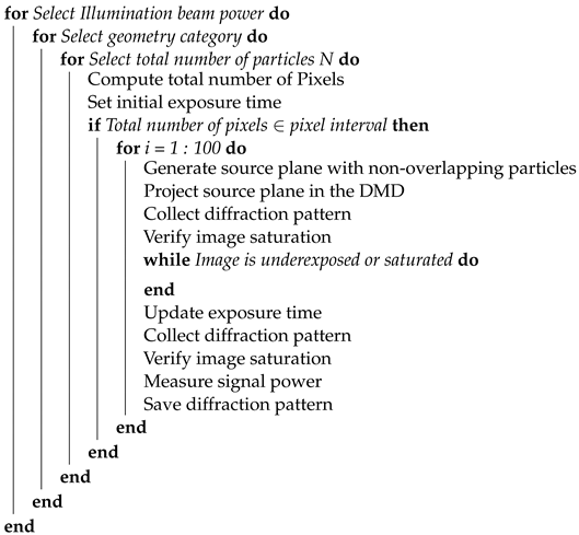
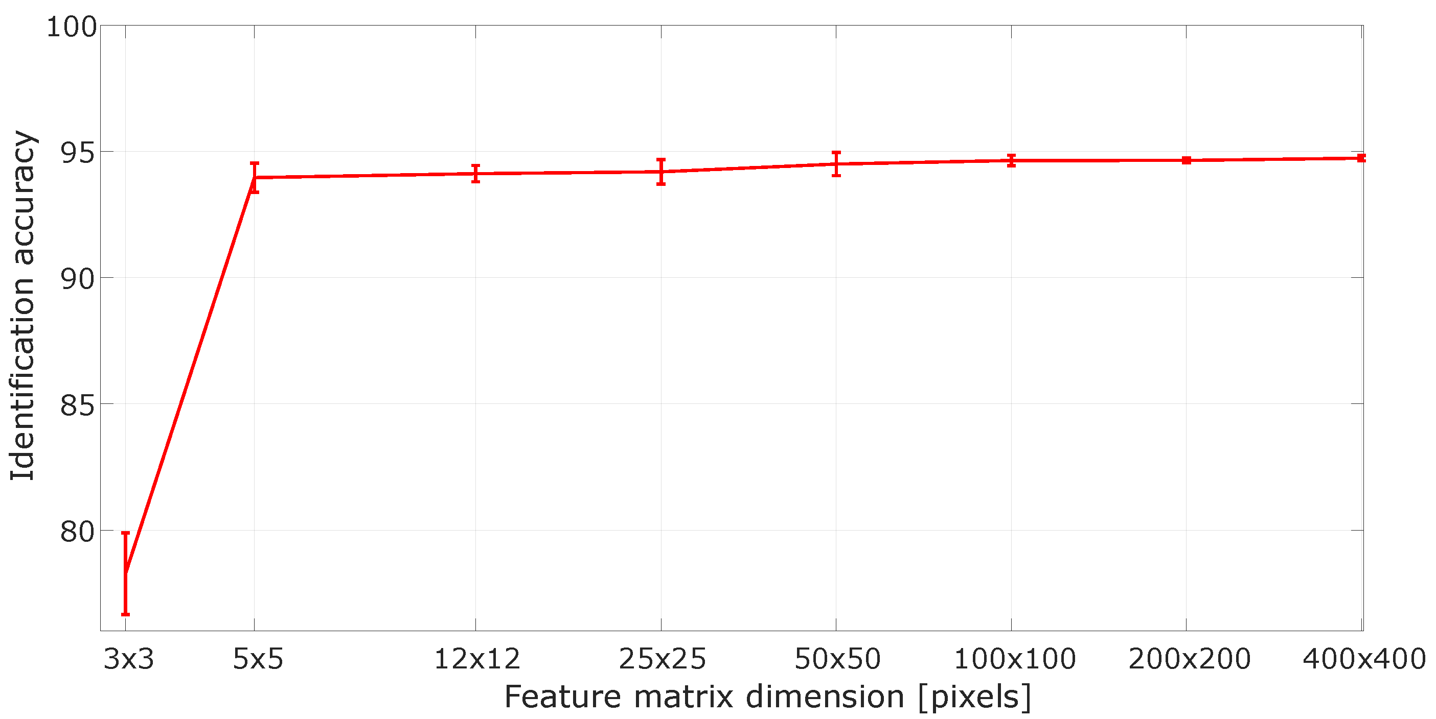
2.2. Neural Network Architecture and Processing

All the algorithms used in our protocol are based on multi-layer feed-forward networks [47]. Hidden layers feature neurons that perform operations on the data using synaptic weights and a nonlinear activation function, the so-called sigmoid function. The output layer comprises softmax neurons that provide a probability distribution over predicted output classes [48,49]. To build accurate and reliable neural networks, a crucial step is to determine an appropriate feature vector that may capture the information encoded in the diffraction patterns. Figure 2b shows the image pre-processing method carried out to build the feature vector. We first crop the diffraction pattern to a $400\times 400$ pixel image, retaining only the central portion of the monochromatic high-resolution original images ($1280\times 1024$ pixels, normalized to 8 bits) obtained with a CCD camera (Thorlabs DCU224C). After this step, to reduce the data dimensions, we perform a down-sampling process that averages small clusters of 80 by 80 pixels, resulting in a 5-by-5 pixel image. It is worth mentioning that we have tested our algorithms with a larger set of features (pixels) without observing a significant efficiency improvement, as shown in Figure 4. The values of identification accuracy that correspond to each one of the feature matrix dimensions are: 78.41 ± 1.94, 94.12 ± 0.75, 94.24 ± 0.65, 94.48 ± 0.41, 94.45 ± 0.32, 94.55 ± 0.2, 94.6 ± 0.12 and 94.77 ± 0.1 (all values correspond to accuracy percentage). Finally, we rearrange the resulting intensity distribution as a column vector, with the total measured intensity included as a 26th element of the resulting feature vector $V_1$, depicted by the red rectangle in Figure 2c.

Our neural networks undergo two stages, namely training, and testing. We train the classification networks using the scaled conjugate gradient back-propagation algorithm [50], while the performance is evaluated through the cross-entropy [51,52]. We devote 70% of the dataset to training, 15% to validation, and 15% to testing, as is standard in ML protocols [53,54]. In all cases, the training of the neural networks was carried out with balanced data, that is, the training dataset contains the same number of observations for each one of the classes. It is worth mentioning that the testing data was excluded from the training phase, thus providing an unbiased evaluation of the algorithm’s overall accuracy. A limit of 1000 epochs was set for each network training stage. Both training and testing stages were performed with MATLAB 2019a which runs on a computer with an Intel Core i7-4710MQ CPU (@2.50 GHz) and 32 GB of RAM. After the training stage, our networks can make predictions of the shape, size, and the number of microscopic objects in a given sample using as input the diffraction pattern and the total intensity, as shown in Figure 2c. In what follows, we provide a thorough description of the steps followed in each experiment.

In Experiment #1, we implement three neural networks connected in series, each one of them performing a specific prediction of the features of the initial field. The first neural network identifies the shape of the objects. It is trained by using a concatenation of the total intensity (signal power) and the down-sampled representation of the diffraction pattern, i.e., the feature vector $V_1$ [see Figure 2b]. The second network, identifying the object size, makes use of the prediction of the first network to create the feature vector $V_2=V_1$ + geometry (shape), whereas the third network extracts the object number from the feature vector $V_3=V_2$ + size. Figure 2c summarizes the structure of the neural networks and the predicted classes. The core feature-vector $V_1$ is initially introduced in the network that identifies the shape. Then, its output acts as input for the second network, in conjunction with the core feature vector. Once the object size has been determined, the third neural network predicts the number of objects using as input the core feature-vector, as well as the outputs of the first and second networks.

In Experiment #2, we follow a similar strategy. We first implement a neural network that determines the combined-geometry (shape) class—i.e., the two shapes of the objects which make up the mixture—by using the feature vector, comprising the down-sampled diffraction pattern and the total measured intensity. With the geometry-class identified and the core feature-vector, we then determine the total number of objects. Finally, by making use of the core feature-vector, as well as the outputs of the first and second networks, we predict the dominant shape. Note that the last network has been divided into two cases: odd and even number of objects. This is due to the fact that when the number of objects is even, we need to define three output classes depending on the concentration ratio, namely (1) larger number of the first geometry, (2) larger number of the second geometry, (3) equal number of model particles of both geometries. For an odd number of objects, there are only two classes. Also note that the class labeled as Geometry-1 (Geometry-2) in Figure 2 refers to the first (second) object-shape in each of classes 1, 2, and 3. It is important to note that in both experiments, all of the data which serves as input to the neural network (both for training and for evaluation), is obtained experimentally through far-field diffraction.

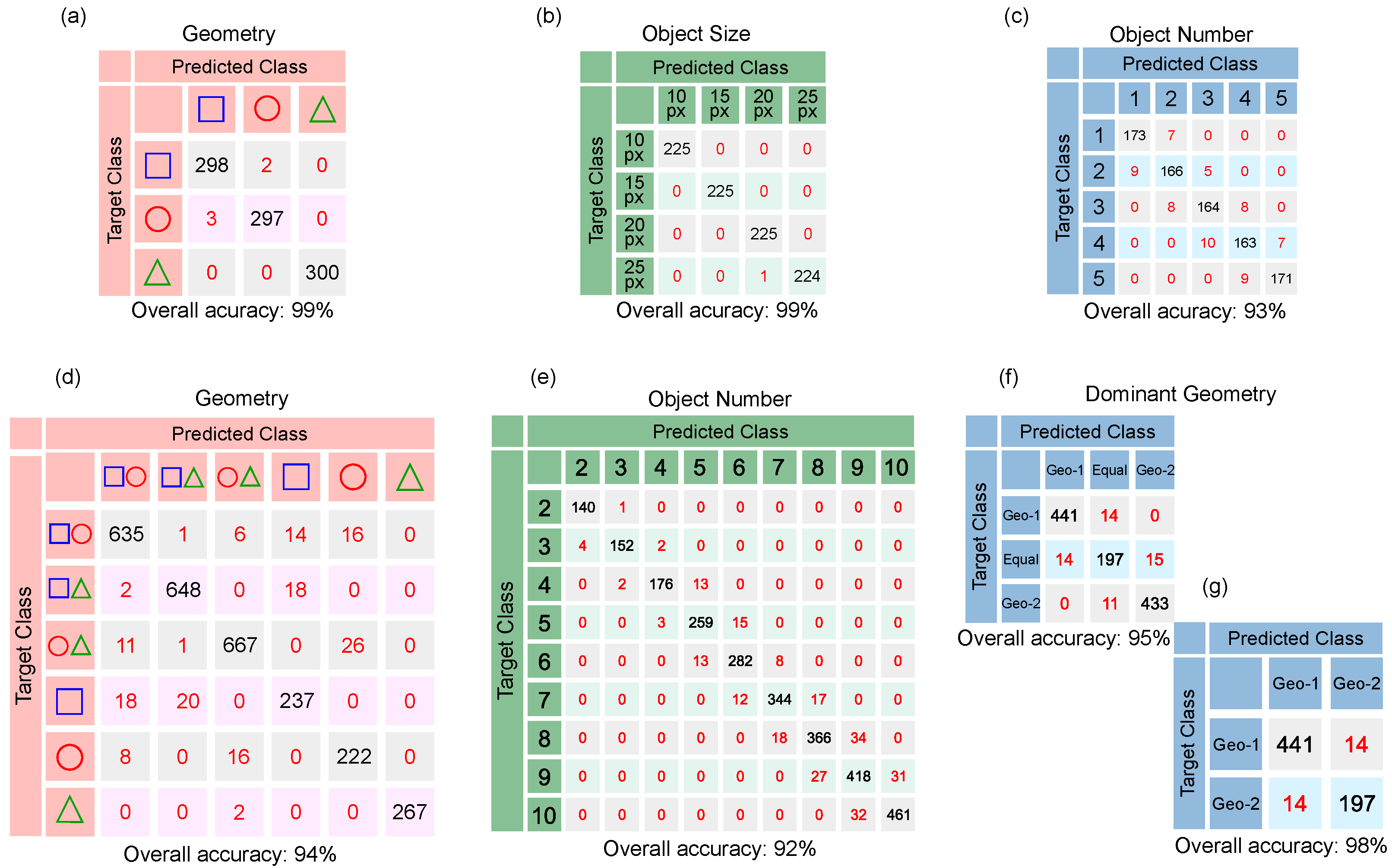
3. Results and Discussion

We have performed a blind test of our neural networks on the remaining 15% of the collected data. We obtain an overall >90% identification accuracy in every stage of the experiments.

Table 2. Overall accuracy, number of hidden layers, and number of neurons in each layer for the neural networks implemented in the described experiments.

Experiment	Neural Network	Accuracy	Number of Hidden Layers	Number of Neurons by Layer
1	Geometry	99%	1	5
	Object Size	99%	1	5
	Object Number	93%	2	Layer 1 = 20; Layer 2 = 5
2	Geometry	94%	2	Layer 1 = 30; Layer 2 = 20
	Object Number	92%	2	Layer 1 = 80; Layer 2 = 50
	Dominant geometry (even)	95%	2	Layer 1 = 30; Layer 2 = 20
	Dominant geometry (odd)	98%	2	Layer 1 = 30; Layer 2 = 20

summarizes the results of each experiment (see Figure 5 for details on the network success rate for each task), including the overall accuracy, the number of hidden layers, and the number of neurons in each layer.

In Experiment #1, featuring collections of one single type (shape) of particle, the first NN can identify the shape of the model particles with a 99% accuracy using a single hidden layer with 5 neurons. The second NN for the determination of particle size showed the same performance, with the same architecture. For the case of the particle number, the architecture of the NN involves two hidden layers with 20 and 5 neurons, respectively, resulting in a 93% identification accuracy.

We remark that in experiment #1 which involves collections of a single type of particle, each one randomly positioned, we can obtain information about particle shape, size, and total number from inputting a single diffraction pattern to our three cascaded NNs, in contrast to other schemes which analyze each particle on a one-by-one basis [25,26].

For experiment #2, featuring heterogeneous mixtures of two types (shapes) of particles, our NN uses two hidden layers. The shape of the particles was retrieved with 94% accuracy using 30 and 20 neurons, respectively; while for the total number of model particles, 80 and 50 neurons were needed for an identification accuracy of 92%. Finally, two layers with 30 and 20 neurons were required to determine the dominant shape obtaining 95% accuracy for the even total number of particles and 98% for the odd number of particles.

We measured the execution time in both training and test stages to quantify the computational cost in terms of the processing time.

Table 3. Computation time for test and training of the neural networks used in each experiment.

Experiment	Neural Network	Training [s]	Test [s]
1	Geometry	$2.308\times {10}^{-1}$ ± $2.7\times {10}^{-3}$	$7.1\times {10}^{-3}$ ± $6.7\times {10}^{-7}$
	Object Size	$2.491\times {10}^{-1}$ ± $4.7\times {10}^{-3}$	$7\times {10}^{-3}$ ± $5.2\times {10}^{-7}$
	Object Number	$3.905\times {10}^{-1}$ ± $9.9\times {10}^{-3}$	$7.2\times {10}^{-3}$ ± $2\times {10}^{-7}$
2	Geometry	4.7212 ± $7.471\times {10}^{-1}$	$1.2\times {10}^{-2}$ ± $1.4\times {10}^{-6}$
	Object Number	$1.57444\times {10}^1$± 4.6636	$1.82\times {10}^{-2}$ ± $2.4\times {10}^{-6}$
	Dominant geometry (even)	1.045 ± $6.1\times {10}^{-2}$	$2.7\times {10}^{-5}$ ± $9.9\times {10}^{-10}$
	Dominant geometry (odd)	$9.513\times {10}^1$ ± $6.5\times {10}^{-2}$	$2.1\times {10}^{-5}$ ± $2.7\times {10}^{-9}$

shows a comparison of the execution time for all the proposed neural networks. Note that, in general, while our algorithms require less than 30 s to be trained, the test time is significantly less than that of the training, around a few tens of milliseconds.

It is worth mentioning that although the data preparation and processing can be considerably time-consuming, once the training phase has been completed, our neural network can process newly-acquired data (prepared in the same format as used for training) in timescales of milliseconds.

4. Conclusions

We have demonstrated an optical technique for particle mixture identification, with potential applications in research and industry, based on machine-learning-assisted laser diffraction analysis. The technique proposed facilitates a fast and accurate identification of the particle’s shape, size, and total number in the case of collections of a single particle type (shape). Likewise, it leads to fast and accurate identification of the geometry of constituent particles, particle size, and dominant geometry in the case of binary non-heterogeneous mixtures. We have verified that the method works detecting arrays of randomly located model particles generated with the help of a DMD. It is worth pointing out that machine learning and deep learning algorithms have been used to improve optical microscopy [35,55,56,57]. Interestingly, by using neural networks as classifiers or feature extractors, in some cases trained with synthetic data and tested in real measurements, these types of techniques have shown to be effective for impurity recognition in semiconductors [58,59].

In our work, by making use of a digital micromirror device, we have simulated mixtures of particles of different sizes and geometries with a different total number of model particles. By analyzing the resulting far-field diffraction pattern, our neural network algorithm can extract the spatial features of the mixtures. Relying on a total of 24,900 diffraction patterns and a 70/15/15 ratio for training, validation, and testing data, respectively, the identification performance remained above 90%. Because of its reliability and ease of implementation, our technique may be of great importance for different scientific and technological disciplines, as it establishes a new route towards the development of novel smart identification devices for sample classification and particle contamination monitoring.

References

1. Banada, P.P.; Guo, S.; Bayraktar, B.; Bae, E.; Rajwa, B.; Robinson, J.P.; Hirleman, E.D.; Bhunia, A.K. Optical forward-scattering for detection of Listeria monocytogenes and other Listeria species. Biosens. Bioelectron. 2007, 22, 1664–1671. [Google Scholar] [CrossRef] [PubMed]
2. Park, J.E.; Kim, K.; Jung, Y.; Kim, J.H.; Nam, J.M. Metal nanoparticles for virus detection. ChemNanoMat 2016, 2, 927–936. [Google Scholar] [CrossRef]
3. Shekunov, B.Y.; Chattopadhyay, P.; Tong, H.H.Y.; Chow, A.H.L. Particle size analysis in pharmaceutics: Principles, methods and applications. Pharm. Res. 2007, 24, 203. [Google Scholar] [CrossRef] [PubMed]
4. Dhamoon, R.K.; Paplo, H.; Aggarwal, G.; Gupta, M. Particle size characterization-techniques, factors and quality-by-design approach. Int. J. Drug Deliv. 2018, 10, 1–11. [Google Scholar]
5. Robins, M.M. Particle size analysis in food. In Encyclopedia of Analytical Chemistry; Meyers, R.A., McGorring, R.J., Eds.; Wiley Online Library: Hoboken, NJ, USA, 2006. [Google Scholar]
6. Zhang, J.; Liu, D.; Liu, Y.; Yu, Y.; Hemar, Y.; Regenstein, J.M.; Zhou, P. Effects of particle size and aging of milk protein concentrate on the biophysical properties of an intermediate-moisture model food system. Food Biosci. 2020, 37, 100698. [Google Scholar] [CrossRef]
7. Roy, S.; Assafrão, A.; Pereira, S.; Urbach, H. Coherent Fourier scatterometry for detection of nanometer-sized particles on a planar substrate surface. Opt. Express 2014, 22, 13250–13262. [Google Scholar] [CrossRef] [Green Version]
8. Tinke, A.P.; Carnicer, A.; Govoreanu, R.; Scheltjens, G.; Lauwerysen, L.; Mertens, N.; Vanhoutte, K.; Brewster, M.E. Particle shape and orientation in laser diffraction and static image analysis: Size distribution analysis of micrometer sized rectangular particles. Powder Technol. 2008, 186, 154. [Google Scholar] [CrossRef] [Green Version]
9. Imhof, H.K.; Laforsch, C.; Wiesheu, A.C.; Schmid, J.; Anger, P.M.; Niessner, R.; Ivleva, N.P. Pigments and plastic in limnetic ecosystems: A qualitative and quantitative study on microparticles of different size classes. Water Res. 2016, 98, 64–74. [Google Scholar] [CrossRef]
10. Parrish, K.; Fahrenfeld, N. Microplastic biofilm in fresh-and wastewater as a function of microparticle type and size class. Environ. Sci. Water Res. Technol. 2019, 5, 495–505. [Google Scholar] [CrossRef]
11. Brown, D.M.; Wilson, M.R.; MacNee, W.; Stone, V.; Donaldson, K. Size-dependent proinflammatory effects of ultrafine polystyrene particles: A role for surface area and oxidative stress in the enhanced activity of ultrafines. Toxicol. Appl. Pharmacol. 2001, 175, 191–199. [Google Scholar] [CrossRef] [Green Version]
12. Oberdörster, G.; Finkelstein, J.; Johnston, C.; Gelein, R.; Cox, C.; Baggs, R.; Elder, A. Acute pulmonary effects of ultrafine particles in rats and mice. Res. Rep. 2000, 96, 5–74. [Google Scholar]
13. Merkus, H.G. Particle Size Measurements: Fundamentals, Practice, Quality; Springer: Berlin/Heidelberg, Germany, 2009. [Google Scholar]
14. Malvern Ltd. A Basic Guide to Particle Characterization; Malvern Ltd.: Malvern, UK, 2015. [Google Scholar]
15. Xu, R. Light scattering: A review of particle characterization applications. Particuology 2015, 18, 11–21. [Google Scholar] [CrossRef]
16. Bradley Deutsch, B.; Beams, R.; Novotny, L. Nanoparticle detection using dual-phase interferometry. Appl. Opt. 2010, 49, 4921–4925. [Google Scholar] [CrossRef] [PubMed] [Green Version]
17. Stetefeld, J.; McKenna, S.A.; Patel, T.R. Dynamic light scattering: A practical guide and applications in biomedical sciences. Biophys. Rev. 2016, 8, 409. [Google Scholar] [CrossRef] [PubMed]
18. Rawle, A. Basic Principles of Particle Size Analysis; Malvern Instruments: Malvern, UK, 1995. [Google Scholar]
19. ISO 13320:2020; Particle Size Analysis—Laser Diffraction Methods. ISO: Geneva, Switzerland, 2020.
20. Blott, S.J.; Croft, D.J.; Pye, K.; Saye, S.E.; Wilson, H.E. Particle size analysis by laser diffraction. Geol. Soc. Lond. Spec. Publ. 2004, 232, 63. [Google Scholar] [CrossRef]
21. Chen, J.; Clay, N.E.; Park, N.h.; Kong, H. Non-spherical particles for targeted drug delivery. Chem. Eng. Sci. 2015, 125, 20–24. [Google Scholar] [CrossRef] [Green Version]
22. Cooley, M.; Sarode, A.; Hoore, M.; Fedosov, D.A.; Mitragotri, S.; Sen Gupta, A. Influence of particle size and shape on their margination and wall-adhesion: Implications in drug delivery vehicle design across nano-to-micro scale. Nanoscale 2018, 10, 15350–15364. [Google Scholar] [CrossRef] [PubMed]
23. Ting, J.M.; Meachum, L.; Rowell, J.D. Effect of particle shape on the strength and deformation mechanisms of ellipse-shaped granular assemblages. Eng. Comput. 1995, 12, 99–108. [Google Scholar] [CrossRef]
24. Zou, R.; Yu, A.B. Evaluation of the packing characteristics of mono-sized non-spherical particles. Powder Technol. 1996, 88, 71–79. [Google Scholar] [CrossRef]
25. Ma, Z.; Merkus, H.G.; de Smet, J.G.; Heffels, C.; Scarlett, B. New developments in particle characterization by laser diffraction: Size and shape. Powder Technol. 2000, 111, 66–78. [Google Scholar] [CrossRef]
26. Ma, Z.; Merkus, H.G.; Scarlett, B. Extending laser diffraction for particle shape characterization: Technical aspects and application. Powder Technol. 2001, 118, 180–187. [Google Scholar] [CrossRef]
27. Blott, S.J.; Pye, K. Particle shape: A review and new methods of characterization and classification. Sedimentology 2008, 55, 31–63. [Google Scholar] [CrossRef]
28. Hentschel, M.L.; Page, N.W. Selection of descriptors for particle shape characterization. Part. Part. Syst. Charact. Meas. Descr. Part. Prop. Behav. Powders Disperse Syst. 2003, 20, 25–38. [Google Scholar] [CrossRef]
29. Hovenier, J.; Lumme, K.; Mishchenko, M.; Voshchinnikov, N.; Mackowski, D.; Rahola, J. Computations of scattering matrices of four types of non-spherical particles using diverse methods. J. Quant. Spectrosc. Radiat. Transf. 1996, 55, 695–705. [Google Scholar] [CrossRef]
30. Mishchenko, M.I.; Travis, L.D.; Mackowski, D.W. T-matrix computations of light scattering by nonspherical particles: A review. J. Quant. Spectrosc. Radiat. Transf. 1996, 55, 535–575. [Google Scholar] [CrossRef]
31. Jia, R.; Zhang, X.; Cui, F.; Chen, G.; Li, H.; Peng, H.; Cao, Z.; Pei, S. Machine-learning-based computationally efficient particle size distribution retrieval from bulk optical properties. Appl. Opt. 2020, 59, 7284–7291. [Google Scholar] [CrossRef] [PubMed]
32. Altman, L.E.; Grier, D.G. CATCH: Characterizing and tracking colloids holographically using deep neural networks. J. Phys. Chem. B 2020, 124, 1602–1610. [Google Scholar] [CrossRef] [Green Version]
33. Daniels, A.L.; Calderon, C.P.; Randolph, T.W. Machine learning and statistical analyses for extracting and characterizing “fingerprints” of antibody aggregation at container interfaces from flow microscopy images. Biotechnol. Bioeng. 2020, 117, 3322–3335. [Google Scholar] [CrossRef]
34. Hundal, H.; Rohani, S.; Wood, H.; Pons, M. Particle shape characterization using image analysis and neural networks. Powder Technol. 1997, 91, 217–227. [Google Scholar] [CrossRef]
35. Rivenson, Y.; Koydemir, H.C.; Wang, H.; Wei, Z.; Ren, Z.; Gunaydın, H.; Zhang, Y.; Gorocs, Z.; Liang, K.; Tseng, D.; et al. Deep Learning Enhanced Mobile-Phone Microscopy. ACS Photonics 2018, 5, 2354. [Google Scholar] [CrossRef]
36. Nascimento, C.; Guardani, R.; Giulietti, M. Use of neural networks in the analysis of particle size distributions by laser diffraction. Powder Technol. 1997, 90, 89–94. [Google Scholar] [CrossRef]
37. Hewitt, C.F.; Whalley, P.B. Advanced optical instrumentation methods. Int. J. Multiphase Flow 1980, 6, 139. [Google Scholar] [CrossRef]
38. Kang, S.; Lyoo, P.; Kim, D.; Park, J. Laser diffraction pattern analysis of various two-dimensional regular-shaped model particles. Adv. Powder Technol. 1994, 5, 33–42. [Google Scholar] [CrossRef]
39. Yevick, A.; Hannel, M.; Grier, D.G. Machine-learning approach to holographic particle characterization. Opt. Express 2014, 22, 26884. [Google Scholar] [CrossRef] [PubMed]
40. Hannel, M.D.; Abdulali, A.; O’Brien, M.; Grier, D.G. Machine-learning techniques for fast and accurate feature localization in holograms of colloidal particles. Opt. Express 2018, 26, 15221–15231. [Google Scholar] [CrossRef] [PubMed] [Green Version]
41. Helgadottir, S.; Argun, A.; Volpe, G. Digital video microscopy enhanced by deep learning. Optica 2019, 6, 506. [Google Scholar] [CrossRef] [Green Version]
42. Kolenov, D.; Pereira, S. Machine learning techniques applied for the detection of nanoparticles on surfaces using coherent Fourier scatterometry. Opt. Express 2020, 28, 19163–19186. [Google Scholar] [CrossRef]
43. Hussain, R.; Noyan, M.A.; Woyessa, G.; Marín, R.R.R.; Martinez, P.A.; Mahdi, F.M.; Finazzi, V.; Hazlehurst, T.A.; Hunter, T.N.; Coll, T.; et al. An ultra-compact particle size analyser using a CMOS image sensor and machine learning. Light Sci. Appl. 2020, 9, 21. [Google Scholar] [CrossRef] [Green Version]
44. Guardani, R.; Nascimento, C.; Onimaru, R. Use of neural networks in the analysis of particle size distribution by laser diffraction: Tests with different particle systems. Powder Technol. 2002, 126, 42–50. [Google Scholar] [CrossRef]
45. Kolenov, D.; Davidse, D.; Le Cam, J.; Pereira, S. Convolutional neural network applied for nanoparticle classification using coherent scatterometry data. Appl. Opt. 2020, 59, 8426–8433. [Google Scholar] [CrossRef]
46. Perez-Leija, A.; Guzman-Silva, D.; de J. León-Montiel, R.; Grafe, M.; Heinrich, M.; Moya-Cessa, H.; Busch, K.; Szameit, A. Endurance of quantum coherence due to particle indistinguishability in noisy quantum networks. npj Quantum Inf. 2018, 4, 45. [Google Scholar] [CrossRef] [Green Version]
47. Svozil, D.; Kvasnicka, V.; Pospichal, J. Introduction to multi-layer feed-forward neural networks. Chemom. Intell. Lab. Syst. 1997, 39, 43–62. [Google Scholar] [CrossRef]
48. Goodfellow, I.; Bengio, Y.; Courville, A. Deep Learning; MIT Press: Cambridge, MA, USA, 2016; Available online: http://www.deeplearningbook.org (accessed on 19 December 2021).
49. Bishop, C.M. Pattern Recognition and Machine Learning; Springer: Berlin/Heidelberg, Germany, 2006. [Google Scholar]
50. Møller, M.F. A scaled conjugate gradient algorithm for fast supervised learning. Neural Netw. 1993, 6, 525–533. [Google Scholar] [CrossRef]
51. Shore, J.; Johnson, R. Properties of cross-entropy minimization. IEEE Trans. Inf. Theory 1981, 27, 472–482. [Google Scholar] [CrossRef] [Green Version]
52. De Boer, P.T.; Kroese, D.P.; Mannor, S.; Rubinstein, R.Y. A tutorial on the cross-entropy method. Ann. Oper. Res. 2005, 134, 19–67. [Google Scholar] [CrossRef]
53. Shebani, A.; Iwnicki, S. Prediction of wheel and rail wear under different contact conditions using artificial neural networks. Wear 2018, 406, 173–184. [Google Scholar] [CrossRef] [Green Version]
54. You, C.; Quiroz-Juárez, M.A.; Lambert, A.; Bhusal, N.; Dong, C.; Perez-Leija, A.; Javaid, A.; de J. León-Montiel, R.; Magaña-Loaiza, O.S. Identification of light sources using machine learning. Appl. Phys. Rev. 2020, 7, 021404. [Google Scholar] [CrossRef]
55. Xing, F.; Xie, Y.; Su, H.; Liu, F.; Yang, L. Deep learning in microscopy image analysis: A survey. IEEE Trans. Neural Netw. Learn. Syst. 2017, 29, 4550–4568. [Google Scholar] [CrossRef]
56. Rivenson, Y.; Göröcs, Z.; Günaydin, H.; Zhang, Y.; Wang, H.; Ozcan, A. Deep learning microscopy. Optica 2017, 4, 1437–1443. [Google Scholar] [CrossRef] [Green Version]
57. Mennel, L.; Symonowicz, J.; Wachter, S.; Polyushkin, D.K.; Molina-Mendoza, A.J.; Mueller, T. Ultrafast machine vision with 2D material neural network image sensors. Nature 2020, 579, 62–66. [Google Scholar] [CrossRef]
58. Nakazawa, T.; Kulkarni, D.V. Wafer map defect pattern classification and image retrieval using convolutional neural network. IEEE Trans. Semicond. Manuf. 2018, 31, 309–314. [Google Scholar] [CrossRef]
59. O’Leary, J.; Sawlani, K.; Mesbah, A. Deep Learning for Classification of the Chemical Composition of Particle Defects on Semiconductor Wafers. IEEE Trans. Semicond. Manuf. 2020, 33, 72–85. [Google Scholar] [CrossRef]
Figure 1. Experimental Setup. A 405 nm laser beam, spatially filtered with two lenses (L1 and L2) and a pinhole (P), is expanded with a telescope system (L3 and L4) to illuminate a Digital Micromirror Device (DMD). The power of the illumination beam can be controlled using a Half-wave Plate (HWP) followed by a Linear Polarizer (LP). The light reflected by the DMD passes through a Fourier transform lens (L5), and the diffraction pattern is collected by a CCD camera at the focal plane of the Fourier lens L5. The power of the signal after L5 was measured using a beam splitter (BS) and a power meter (PM).
Photonics 09 00074 g001
Figure 2. Machine-learning-assisted particle mixture identification. (a) Flowchart of the machine learning algorithms used for extracting information from intensity-only measurements of the diffraction patterns. (b) Image down-sampling process. The intensity signal extracted from the CCD camera is presented in false color for the sake of clarity of the presentation. (c) Flow diagram of the neural networks used in each phase of the experiments described in the main text.
Photonics 09 00074 g002
Figure 3. Diffraction patterns measured in experiments. (a,d,g) show examples of the objects generated with the Digital Micromirror Device (DMD). (b,e,h) are the theoretically predicted diffraction patterns created by the objects depicted in the leftmost column. (c,f,i) are the experimentally measured diffraction pattern. Note that the images are normalized, so that the integrated signal over the detection area adds up to unity. In all cases, the overlap parameter Ω is found to be larger than 0.9 .
Photonics 09 00074 g003
Figure 4. Identification accuracy as a function of the feature matrix dimension. Error bars indicate standard deviations.
Photonics 09 00074 g004
Figure 5. Confusion matrices that summarize the performance of machine-learning algorithms for particle mixture identification. The top row shows the confusion matrices containing information about the correct and incorrect predictions for (a) geometry (shape), (b) model particle characteristic size, and (c) number of objects of the Experiment #1. The bottom row presents the confusion matrices for (d) geometry (shape), (e) number of model particles, and (f,g) dominant geometry (shape) of the Experiment #2. (f,g) matrices correspond to the case in which the number of objects is even and odd, respectively. In all cases, the diagonal elements of the matrices represent successful recognition, i.e., true-positives and true-negatives, whereas off-diagonal elements represent failed attempts, false-negatives, and false-positives.
Photonics 09 00074 g005