Abstract
Stray light, such as sunlight, moonlight, and earth-atmosphere light, can bring about light spots in backgrounds, and it affects the star detection of star sensors. To overcome this problem, this paper proposes a star detection algorithm (CMLCM) with multidirectional local contrast based on curvature. It regards the star image as a spatial surface and analyzes the difference in the curvature between the star and the background. It uses a facet model to represent the curvature and calculate the second-order derivatives in four directions. According to the characteristic of the star and the complex background, it enhances the target and suppresses the complex background by a new calculation method of a local contrast map. Finally, it divides the local contrast map into multiple 256 × 256 sub-regions for a more effective threshold segmentation. The experimental results indicated that the CMLCM algorithm could effectively detect a large number of accurate stars under stray light interference, and the detection rate was higher than other compared algorithms with a lower false alarm rate.
1. Introduction
A star sensor [1] is a high-precision attitude measurement device. It is widely used in various space vehicles, including space stations, mars probes, and various satellites in different orbits. However, a spacecraft inevitably encounters various stray light interferences when it is sailing. The most classical case is a satellite orbiting the earth, which is prone to encounter interference from stray light, such as sunlight, moonlight, and earth-atmosphere light [2]. The most obvious feature of these stray lights on the star image is a continuous light spot. The stray light will not only affect the size of the star spot and the energy distribution but also form a light spot on the star image. This interferes with the normal operation of star detection [3,4,5] and affects the attitude measurement accuracy of star sensors. The background with stray light can be called a complex background.
Many experts have conducted research on star detection algorithms of star sensors. Traditional methods include Toggle [6,7] and spatial filtering [8]. However, under complex backgrounds, the extraction accuracy is easily affected by stray light. Therefore, some experts have put forward the background prediction algorithm [9], which can detect stars by calculating vast local thresholds. Moreover, Yu [10] designed a template for background filtering. The connected domain labeling method proposed by Liu [11] is the most widely used method, which can detect the stars of a star map by obtaining the connected domain. However, as shown in Figure 1, when these star extraction algorithms encounter actual complex backgrounds, their ability is greatly reduced.
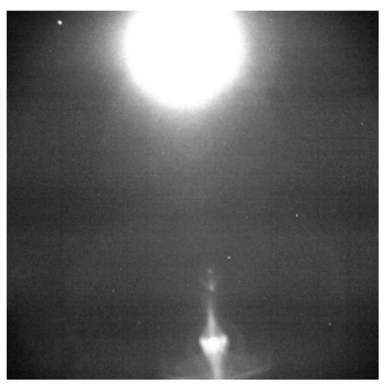
Figure 1.
Stray light in a star image.
Because stars are relatively small after imaging on the target surface of the CMOS detector, their window sizes are usually from to pixels, which gives them the characteristics of a “dim target.” Therefore, this paper not only compares the traditional star extraction algorithm of star sensors but also analyzes the dim target detection method. The traditional dim target detection algorithm includes spatial filtering and frequency-domain filtering [12], which easily cause false detection under complex background interference. Recently, many studies on dim target detection for complex backgrounds have been conducted. Zhao [13] introduced curvature into dim target detection. Prior work [14] proposed an infrared dim target detection algorithm, called ZGQ, based on curvature. At the same time, inspired by the human visual mechanism [15], visual saliency and scale-space theory have attracted extensive attention. Chen [16] proposed a detection algorithm named the local contrast method (LCM) strategy. Subsequently, Han [17] proposed an improved LCM algorithm to improve the detection rate and reduce the false alarm rate, which achieved favorable detection results. Wei [18] proposed a new method called multi-scale patch contrast measurement (MPCM). Lu [19] proposed a first-order curvature-based method (MDWCM) for infrared dim target detection to solve complex background interference on the ground. However, these dim target detection algorithms have limitations and cannot deal with complex backgrounds encountered by star sensors in orbit.
In this paper, a new algorithm for star detection, named curvature-based multidirectional local contrast method (CMLCM), is proposed. The main innovations of this algorithm can be summarized as follows: Firstly, star image is regarded as a spatial surface, and a facet model is used to obtain the second-order derivatives in the four directions of the star image. Because this model provides a fast and accurate fitting of neighborhood images and the calculation of second-order derivatives is relatively simple. Secondly, by combining it with the features of stars and complex backgrounds, a new local contrast enhancement method is proposed. This enhances the local second-order derivatives of stars and weakens the local second-order derivatives of complex backgrounds. Then, the map of second-order derivatives with local contrast enhancement can be obtained. Finally, the local threshold segmentation of patches in the map can be used to detect more useful stars in complex backgrounds. The proposed algorithm was verified by experiments, and the experimental results showed that the proposed CMLCM algorithm could effectively detect a large number of accurate stars under stray light interference. It had a higher detection rate than the other compared algorithms under the same false alarm rate. Moreover, the processing time of the algorithm was close to or lower than the compared algorithms.
2. Materials and Methods
2.1. Calculation of Image Curvature Based on a Facet Model
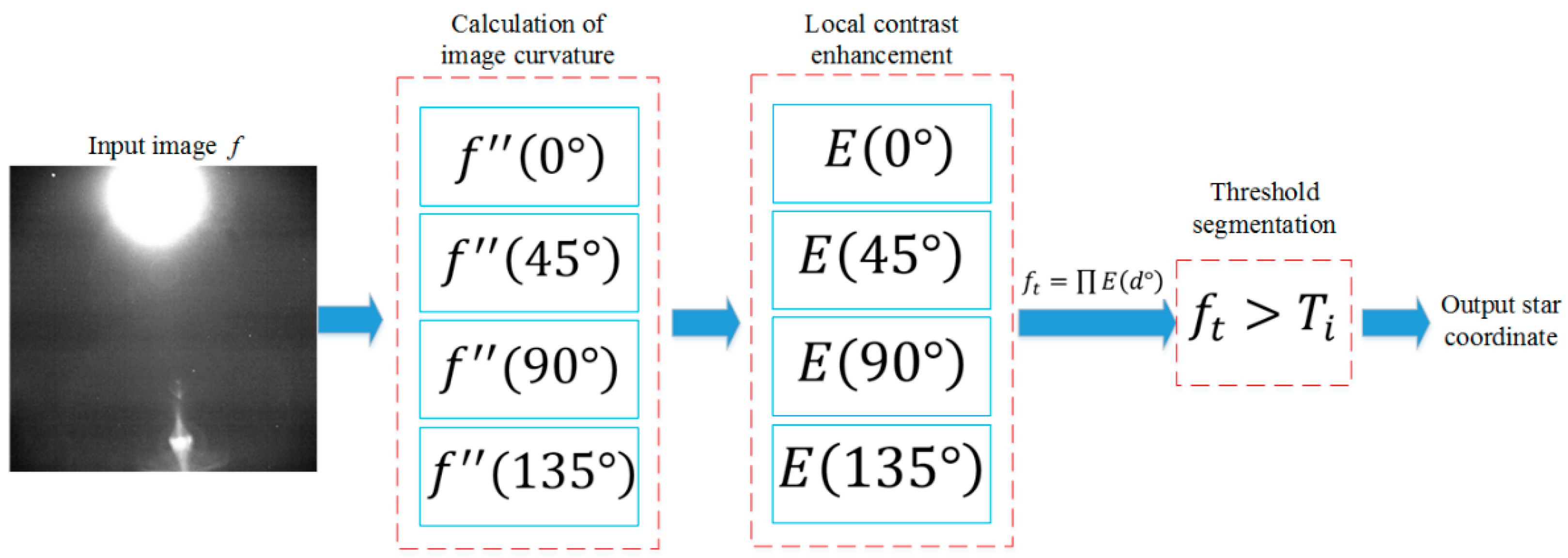
As shown in Figure 2, the first step of CMLCM algorithm is the calculation of image curvature. In the differential theory of unary function, curvature reflects the bending degree of a curve at a certain point. For a point on the curve , if the point has the second-order derivative, the curvature at this point can be expressed as
where represents the curvature at a point , represents the second-order derivative of the curve, and represents the first-order derivative of the curve.
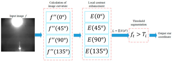
Figure 2.
Flow chart of the CMLCM algorithm.
According to Equation (1), the curvature of a certain point on the image can be expressed as the fusion of the second-order derivative and the first-order derivative in a certain direction. In the discrete condition, the spatial curvature of the point can be characterized by calculating the derivative in the four directions of and .
In this paper, the facet model proposed by Haralick [20] is used to describe the image. It is supposed that R and C are the index set in the symmetric field, where and . The central pixel can be represented by the pixel value in the neighborhood, and it can be expressed as follows:
where is the basis of discrete orthogonal polynomial, and , is the combination coefficient.
Since the values of each pixel in the image are different, according to Equation (2), the expression of the combined coefficient can be obtained by using the orthogonal characteristics of the least square fitting polynomial as follows:
where , and then Equation (4) can be obtained as
Thus, can be expressed as the convolution of the weight coefficient and the image . The results of can be obtained according to the characteristics of .
Combined with the calculation principle of directional derivative, the first-order and second-order derivatives of pixel along with the direction vector can be obtained as follows:
and
where represents the angle between the direction vector and the row direction of image.
Combined with Equations (6) and (7), it can be seen that the complexity in the second-order derivative calculation process will be reduced from 2N to N. Therefore, the second-order derivative is adopted in the subsequent characterization of the image curvature in this paper. The weight coefficient can also be obtained by combining Equations (2)–(4).
The second-order derivative in four directions of and can be obtained according to Equations (7) and (8), which can be used for subsequent calculations.
2.2. Local Contrast Enhancement
The main objective of local contrast enhancement is to enhance the star target and weaken the complex background. The second-order derivative characteristics of the star, flat background, and complex background are analyzed.
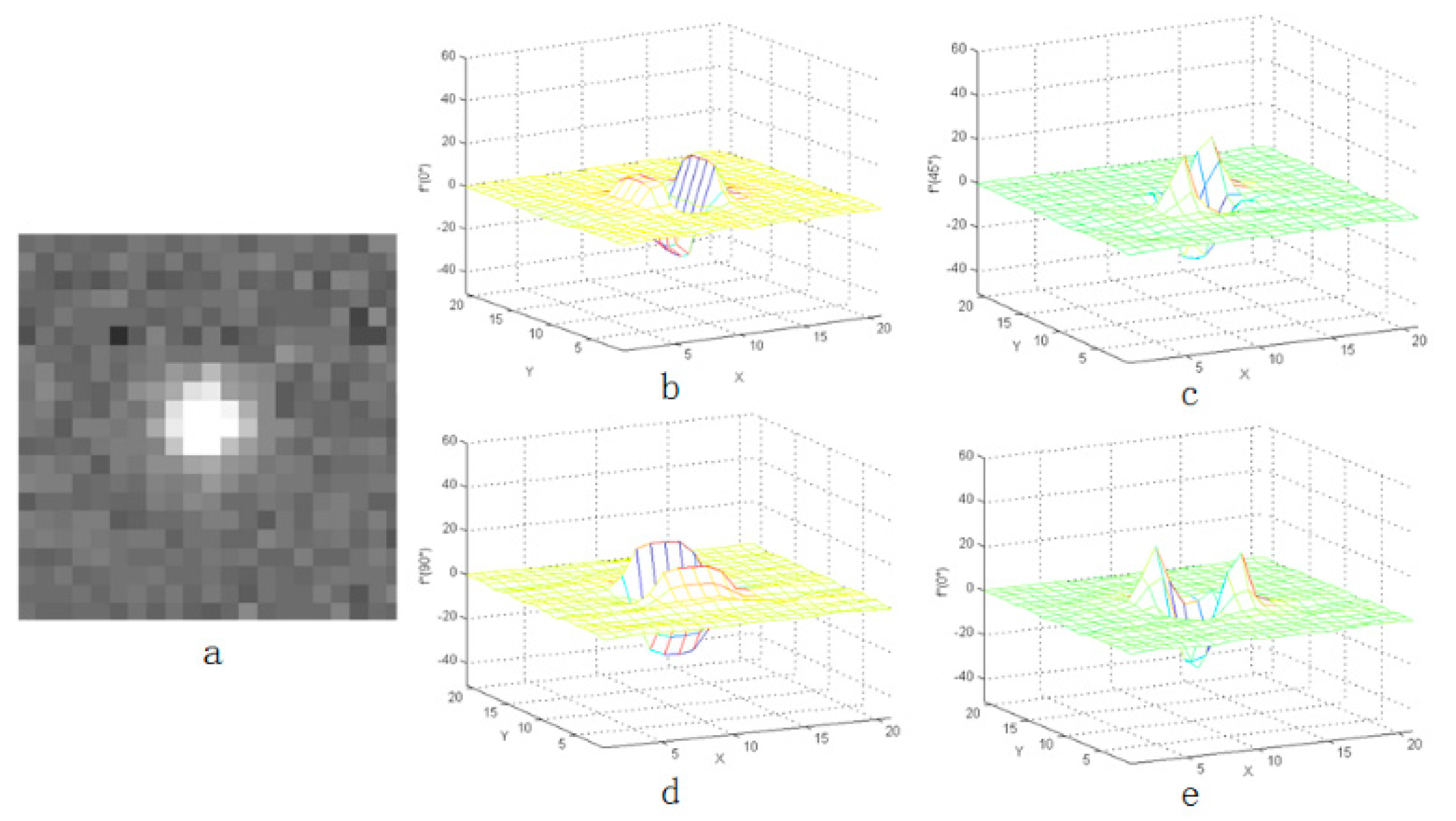
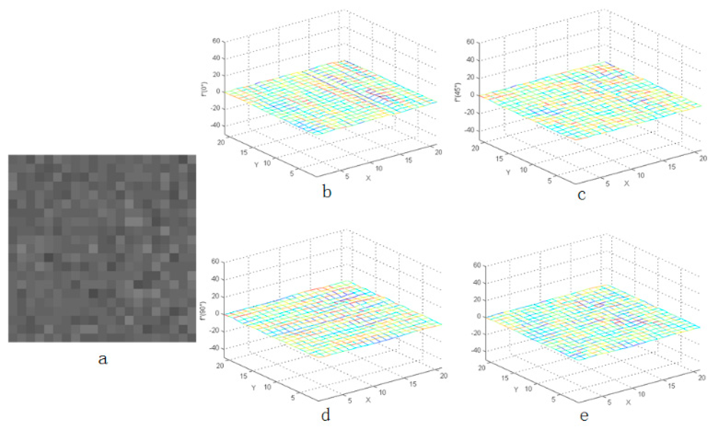
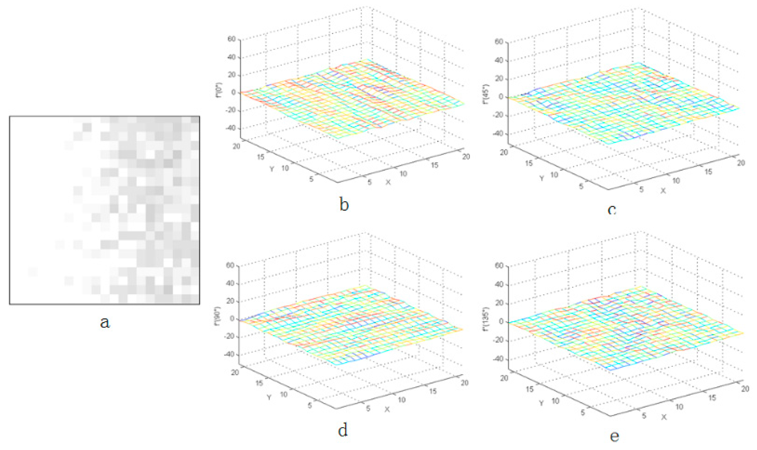
As shown in Figure 3, Figure 4 and Figure 5, the distribution of the second-order derivative of the star in the derivation direction was characterized by the positive peak to the negative peak and then to the positive peak. The non-uniformity noise exists mainly in the star image, and the intensity of non-uniformity noise is not high, which has been verified on orbit. Therefore, after calculating the second-order derivative of star image, the characteristics of noise were not obvious in Figure 3. Besides, the peak characteristics of the second derivative were relatively weak or even gentle in the areas where the flat background or complex background exists. Therefore, the idea of an LCM can be used to enhance the target and weaken the influence of the complex background.
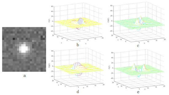
Figure 3.
Second-order derivative characteristics of star in four directions: (a) the star point and (b–e) the three-dimensional distribution of the star point.
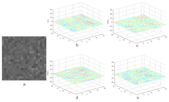
Figure 4.
Second-order derivative characteristics of flat background in four directions: (a) the flat background and (b–e) the three-dimensional distribution of flat background.
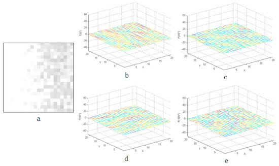
Figure 5.
Second-order derivative characteristics of complex background in four directions: (a) the complex background and (b–e) the three-dimensional distribution of complex background.
In this paper, a better method for local contrast enhancement was designed by combining the second-order derivative values in the four directions.
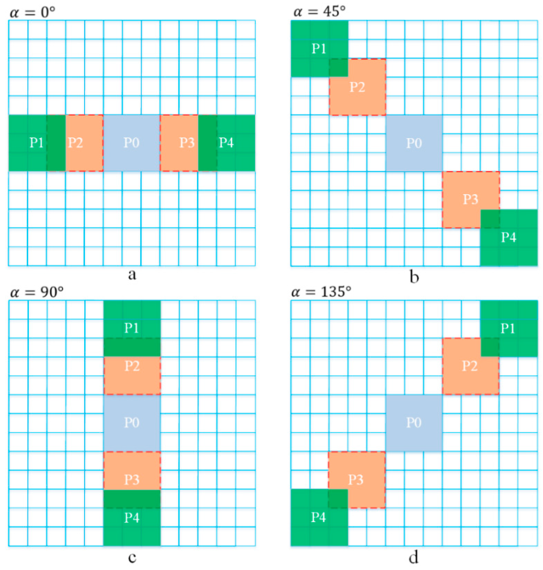
As shown in Figure 6, five local second-order derivative patches, named P0, P1, P2, P3, and P4, were obtained in the four directions of and . The size of each patch is . Here, P0 represents the mean value of the second-order derivative in the middle region, and .
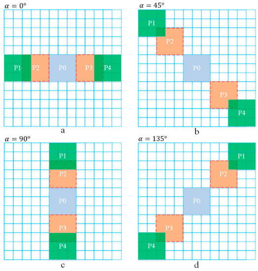
Figure 6.
(a–d) Local second-order derivative in four directions.
The values of P1, P2, P3, and P4 are different in the four directions of and , which can be expressed as
Here, P1, P2, P3, and P4 are mean values of the region when the center pixel is shifted pixel and pixel in the column and row, respectively, where .
As shown in Figure 3, if , then, when the pixel was inside the star, it could be found that the mean value in the central 3 × 3 region was negative. The mean value of surrounding regions is positive.
This can be expressed as follows:
Two adaptable windows are set at the same time to deal with stars of different sizes.
Because the second-order derivative of the star is varying from positive peak value to negative peak value and then to positive peak value, the local contrast of the star can be enhanced using this characteristic.
If and P0, P1, P2, P3, and P4 meet the condition that
then the enhanced local contrast map can be obtained as follows:
where is the attenuation factor of single-pixel noise (the second-order derivative of single-pixel noise was similar to the star, so we add the attenuation factor) as follows:
where
Here, is the pixel value in the position of the star map, and is the central pixel value, and is the mean value of the surrounding eight pixels. The factors weakened the single pixel noise, in which the middle pixel was particularly bright and the surrounding eight pixels are weak.
For the cases where Equation (11) was not satisfied, it was composed of a flat background and stray light, and needed to be weakened by a dividing factor.
Similarly, according to Figure 6, the second-order derivative map can be calculated, where .
Normalization and removal of the negative value for the second-order derivative map were required. The first step was to subtract the negative number.
If , then we set This removed the negative peak value after the second-order derivative operation and retained the local maximum positive peak value.
Then, the normalization operation was carried out and the normalized second-order derivative map could be expressed as
Finally, the product of was used to balance the deviation of the second-order derivative in each direction.
After local contrast enhancement, is obtained as the CMLCM value.
2.3. Block Threshold Segmentation
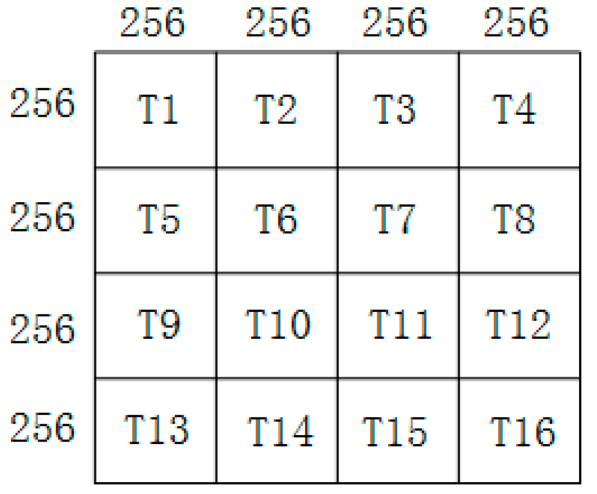
After the CMLCM value was obtained, the technology of block threshold segmentation was used to locate the star position. The whole star image was cut into multiple regions with a size of 256 × 256. The CMLCM mean value and variance of the i-th region was calculated, and the segmentation threshold of the i-th region can be expressed as
As shown in Figure 7, the coordinate position of the star can be extracted after threshold segmentation for each 256 × 256 region.
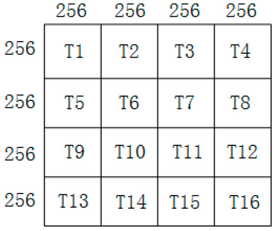
Figure 7.
Block threshold segmentation.
The steps of the CMLCM algorithm are given in Algorithm 1.
| Algorithm 1 CMLCM |
| Input: Original image |
|
Output: |
|
1: Compute four second-order directional derivatives |
|
2: Divide the image patch into 3 × 3 cells |
|
3: Calculate the average value , and of the patches |
|
4: Calculate local contrast ma , |
|
5: Remove the negative and normalization |
| 6: Get the CMLCM value |
3. Results
3.1. Experimental Conditions
The performance of the proposed CMLCM algorithm was evaluated experimentally. The operating platform was a 2.5 GHz Intel I7 CPU with 16 GB of memory, and the simulation software was MATLAB R2012b. The operating system was Windows 7.
Firstly, the influence of noise on real image was analyzed. The random noise was added to the real image when the noise increased from 1% to 80% of the maximum star gray value.
where Q is the coefficient of noise, is the original image, is the image with added random noise. Max means the calculation of maximum value. Rand means the random noise. M and N are the size of image.
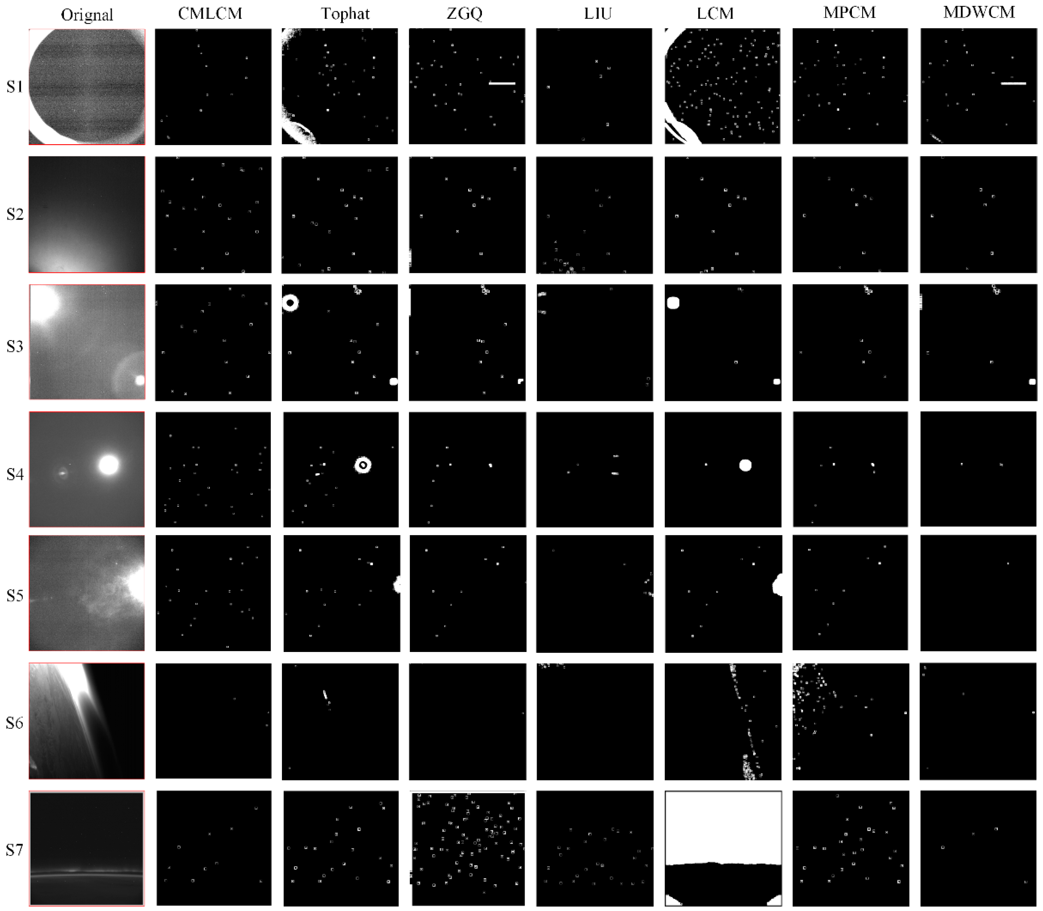
Secondly, the CMLCM was applied to analyze the real image sequences. There were seven real star image sequences (S1–S7) in the experiments. The sequences were the actual star images taken by several models of star sensors in high and low orbits. There was single-pixel noise, moonlight interference, sunlight interference, or earth-atmosphere light interference in the star images. Sequence S1 was the condition when light leaked around the hood, S2 to S5 were the conditions when sunlight and moonlight enter into the field of view, S6 and S7 were the conditions when earth-atmosphere light entered into the field of view. S1 to S7 can actually cover most conditions of complex backgrounds. The proposed CMLCM algorithm was compared with other algorithms, such as TOPHAT [7], ZGQ [14], LIU [11], LCM [16], MPCM [18], and MDWCM [19].
In Section 3.2.2, to compare the difference of star point extraction ability for different algorithms, the star points after extraction were marked in the graph.
In Section 3.2.3, the characteristics of the receiver operating characteristic (ROC) [21] curve were analyzed. In the ROC curve, the horizontal axis represents the false alarm rate and the vertical axis represents the detection rate , which can be expressed as
where represents the actual number of star targets in the star image, represents the number of correctly detected targets, represents the number of targets for error detection, and represents the total number of targets detected by the algorithm (including correct detections and false detections). The actual number and position of star targets in the star image can be calculated by manual mark and searching the star library.
In Section 3.2.4, the CMLCM algorithm was compared with other algorithms to measure the time consumption.
3.2. Experimental Results
3.2.1. The Analysis of the Influence of Noise on the Image
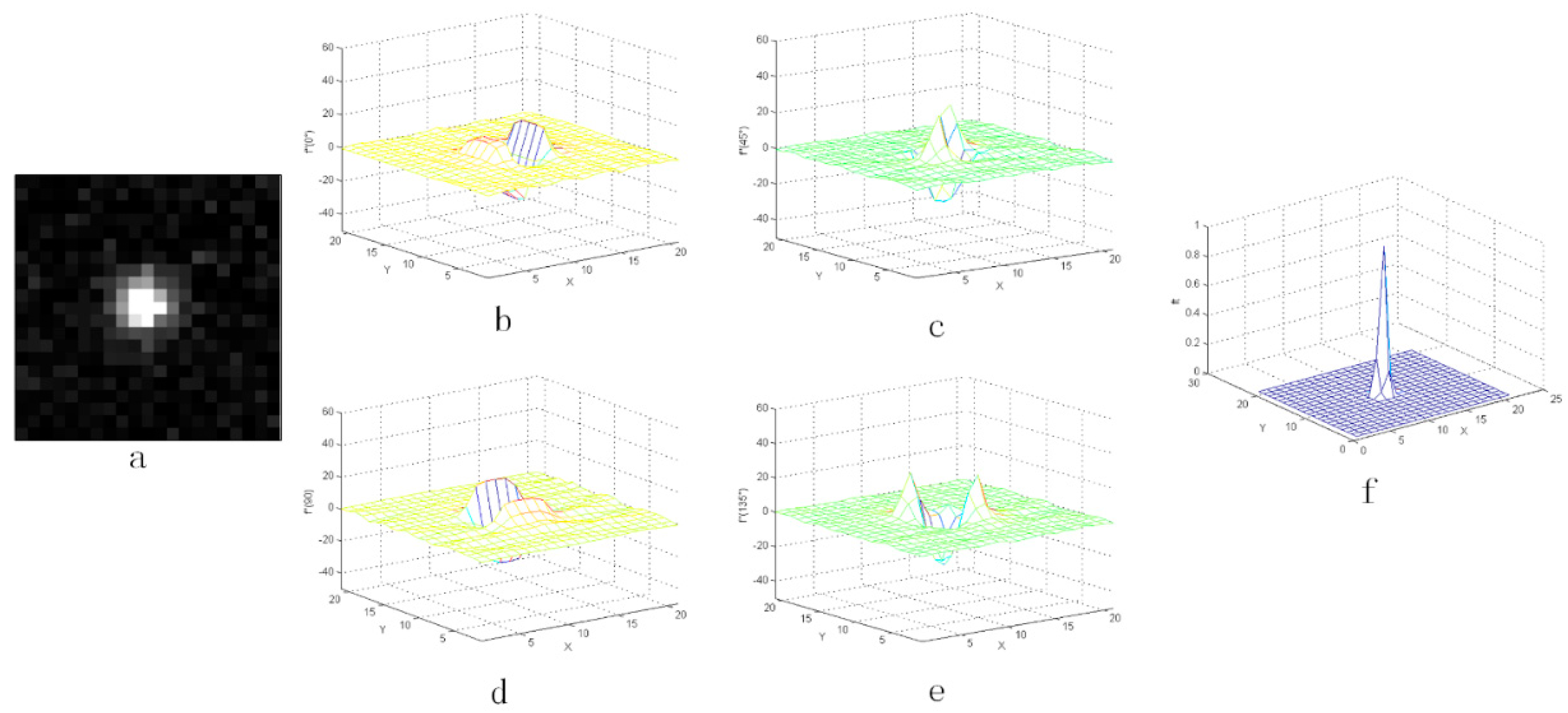
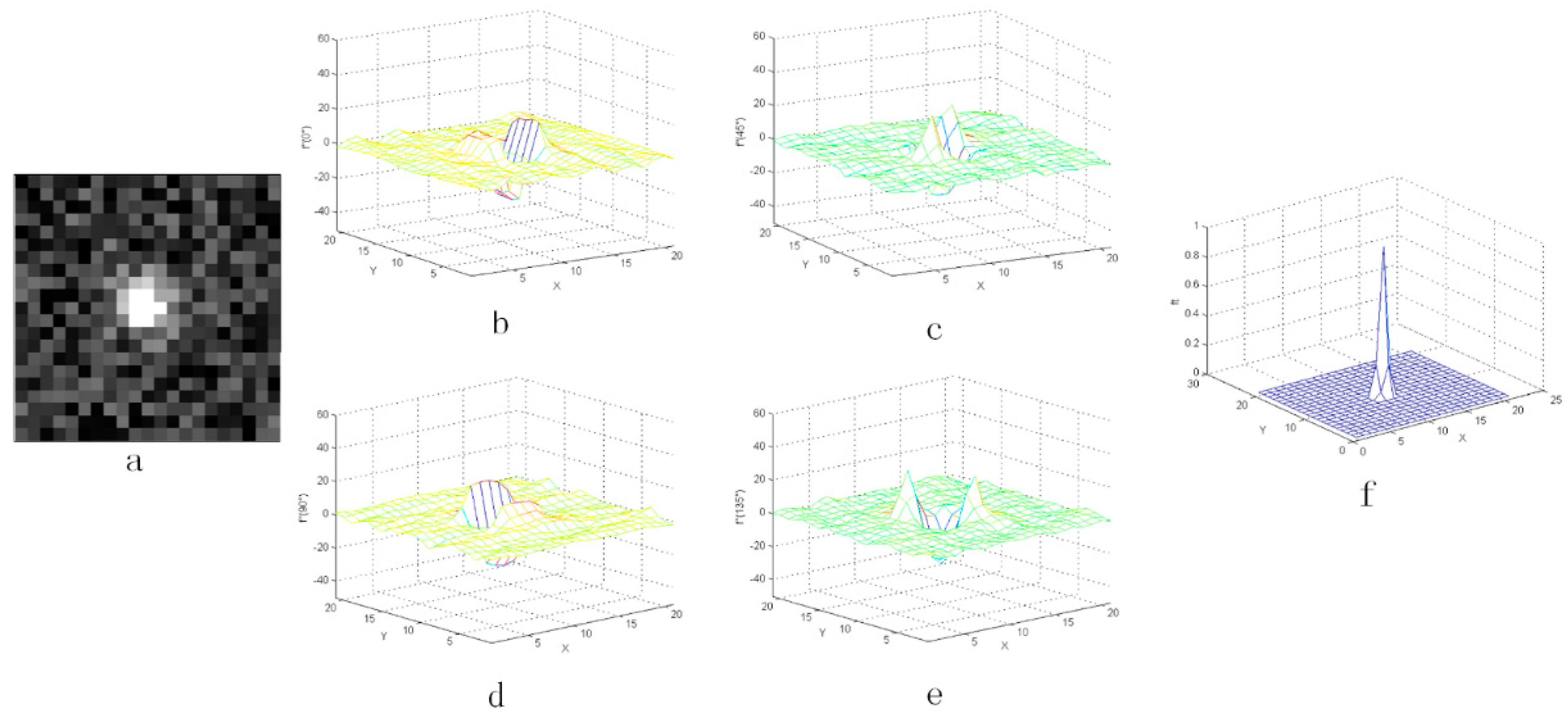
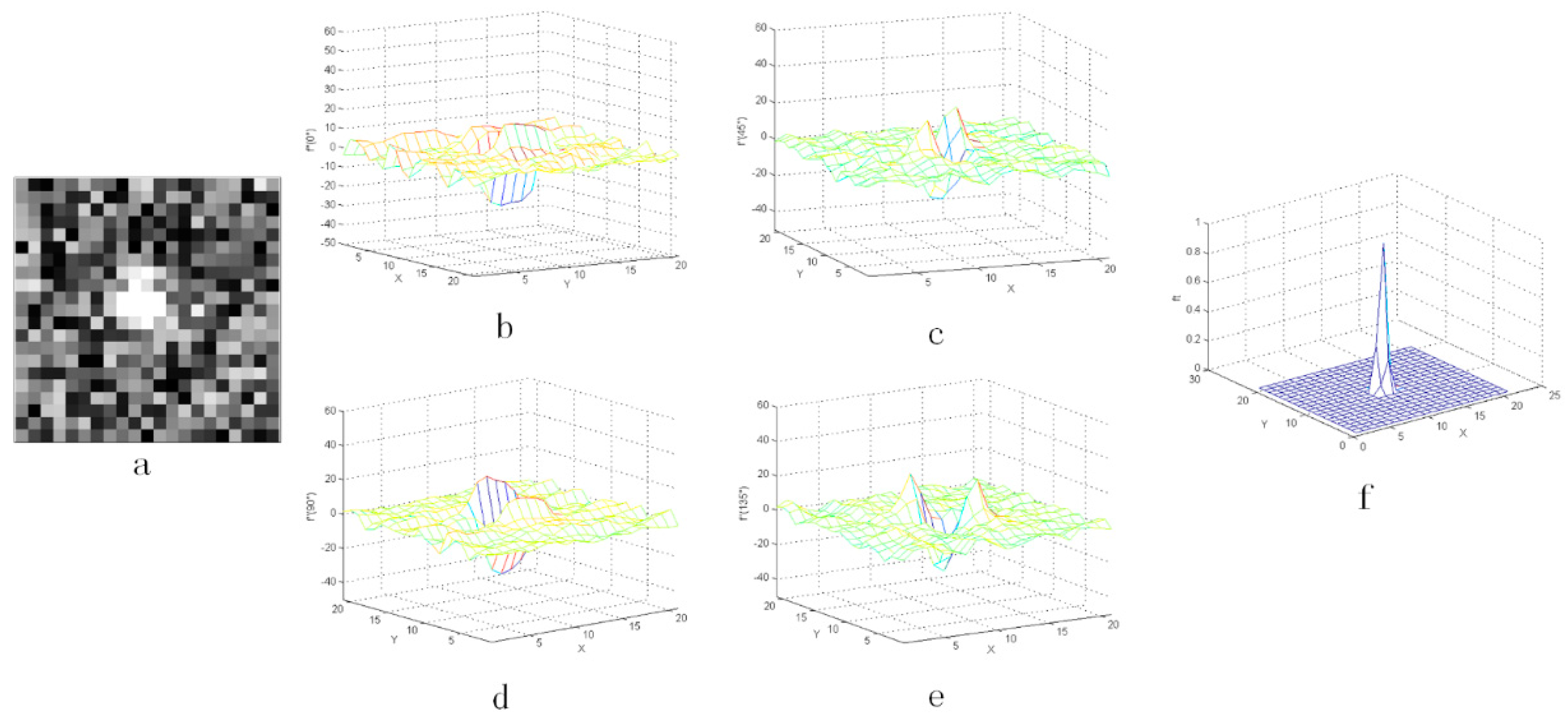
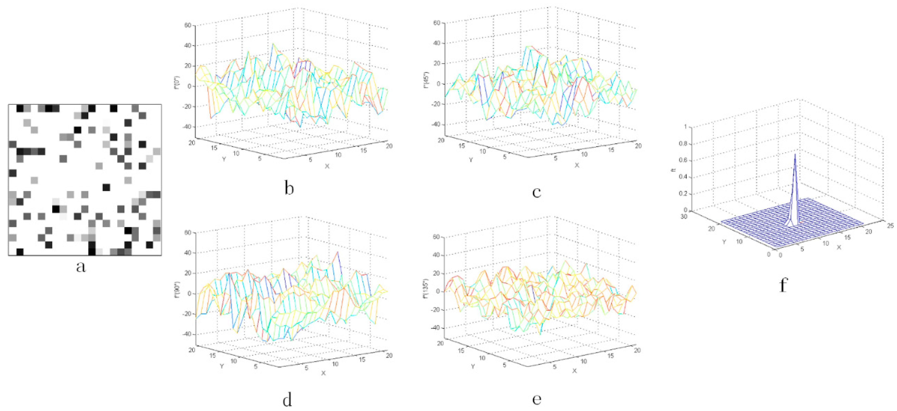
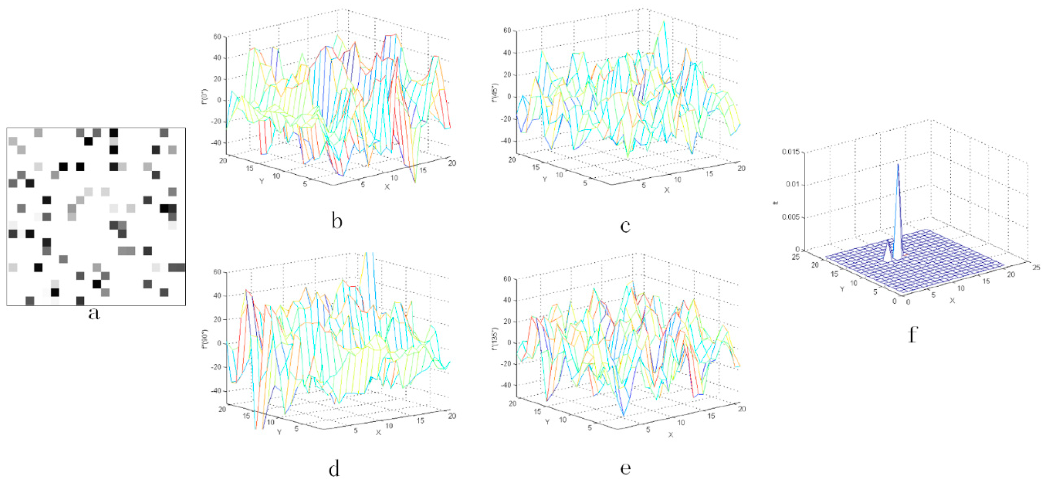
As shown from Figure 8, Figure 9, Figure 10, Figure 11 and Figure 12, when the coefficient Q of noise grew, the three-dimensional distribution of second-order derivative seemed noisier. However, if the coefficient Q of noise was smaller than 50%, the output value locating in the position of star was relatively larger than others around. The star can easily be detected by threshold segmentation. Besides, it can be found that the noise in the actual star image is not serious and the coefficient of noise is usually smaller than 10%. Therefore, it can be concluded that the CMLCM algorithm is not sensitive to noise.
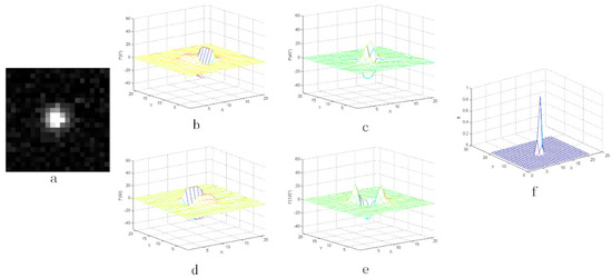
Figure 8.
The result with the noise whose coefficient Q is 1%: (a) the star image with added random noise and (b–e) the three-dimensional distribution of the second-order derivative, (f) the output value after CMLCM processing.

Figure 9.
The result with the noise whose coefficient Q is 5%: (a) the star image with added random noise and (b–e) the three-dimensional distribution of the second-order derivative, (f) the output value after CMLCM processing.

Figure 10.
The result with the noise whose coefficient Q is 10%: (a) the star image with added random noise and (b–e) the three-dimensional distribution of the second-order derivative, (f) the output value after CMLCM processing.
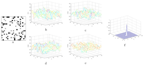
Figure 11.
The result with the noise whose coefficient Q is 50%: (a) the star image with added random noise and (b–e) the three-dimensional distribution of the second-order derivative, (f) the output value after CMLCM processing.
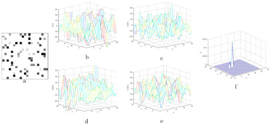
Figure 12.
The result with the noise whose coefficient Q is 80%: (a) the star image with added random noise and (b–e) the three-dimensional distribution of the second-order derivative, (f) the output value after CMLCM processing.
3.2.2. Comparison of the Star Point Extraction Effect
As shown in Figure 13, the proposed CMLCM algorithm and the compared algorithms, TOPHAT, ZGQ, LIU, LCM, MPCM, and MDWCM, were applied to extract the star points from S1 to S7. The first column in Figure 13 is the original input image, and the other columns are the extracted effect of each algorithm. In the figures, all the detected stars (including false stars) are marked with a white box.
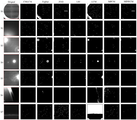
Figure 13.
Comparison of the extraction effects with different algorithms in seven sequences.
As shown in Figure 13, the TOPHAT algorithm had strong detection ability in S2 and S7. This means that weak stray light did not affect the detection ability of the TOPHAT algorithm. However, when stray light occupied a large proportion in the field of view or the gray value of stray light was high, the TOPHAT algorithm easily detected many false stars.
Compared with the TOPHAT algorithm, ZGQ had a great improvement in the suppression of stray light. However, in S3, S4, and S5, when stray light with high energy such as sunlight and moonlight entered the field of view, it was easy to raise the average value of the curvature diagram. Therefore, many correct star points could not be extracted during threshold segmentation, and some false star points were extracted.
Liu used the method of line detection with connected domain calculation to extract stars. It can be found that the relatively bright connected regions caused by stray light were mistakenly detected as stars in S3, S4, and S5. Furthermore, the earth-atmosphere light was easily mistakenly detected as many connected domains when it was distributed in vertical lines. This resulted in many false star targets.
The detection ability of the LCM algorithm was similar to TOPHAT. It was also easy for interference to be caused by sunlight and moonlight. Meanwhile, in S1, it was easy for single-pixel noise to cause interference in the LCM algorithm. Moreover, in S7, many false star points were detected if the energy distribution of stray light was relatively scattered.
In MPCM and MDWCM, there was some improvement in the local contrast enhancement and stray light suppression. In S3, S4, and S5, only a few false stars were extracted in the area of moon or sunlight (MPCM performed better than MDWCM). The number of correct stars was also only a few. However, in S6, the continuous earth-atmosphere light had a great influence on the MPCM algorithm, and there were many false stars after detection.
In contrast, the proposed CMLCM algorithm could effectively detect many accurate stars with the interference of single-pixel noise, moonlight, sunlight, or earth-atmosphere light. It was not susceptible to the interference of complex backgrounds. Only a small quantity of false targets were detected when there existed the small highlighted area in the moonlight (S4), where the small highlighted area had the similar second-order derivative like the star. However, these false stars are easy to be eliminated after the subsequent step of star recognition, which will calculate the angular distance between stars and search them in star library.
3.2.3. Analysis of the Receiver Operating Characteristic Curve
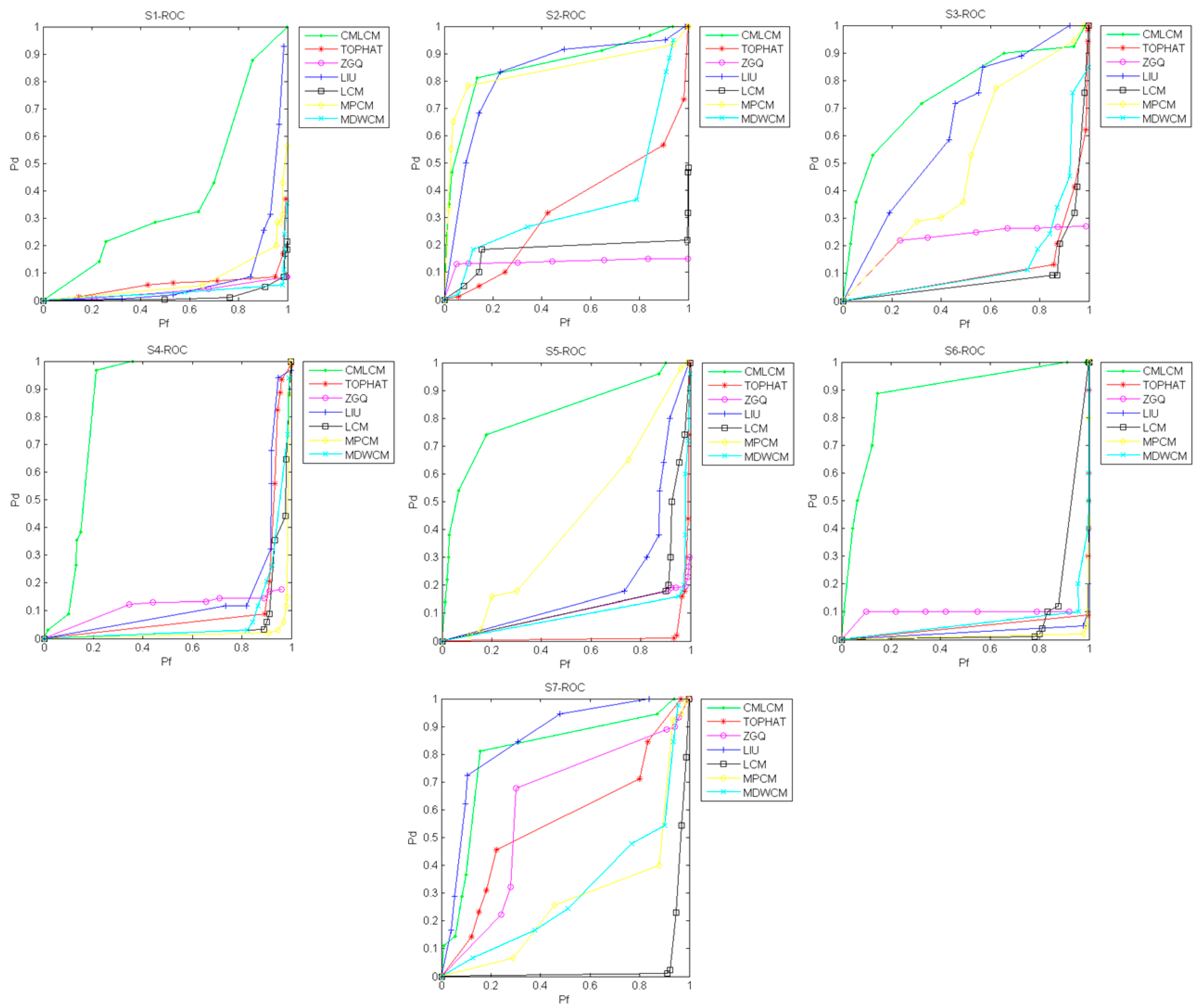
As shown in Figure 14, the ROC curve was calculated for the S1–S7 sequences. In the figure, Pd represents the detection rate ( in Equation (18)) and Pf represents the false alarm rate ( in Equation (18)). A comparison of the algorithms shows that the detection rate of the CMLCM algorithm was higher than the other algorithms when the false alarm rate was the same in most situations. Considering that a star sensor does not need to extract all the stars in the matching process, it could generally achieve perfect matching and attitude measurement with eight to nine correct stars. Therefore, when the ultimate detection rate was not pursued, the CMLCM algorithm could ensure a lower false alarm rate to weaken the effect of false stars in the matching process.
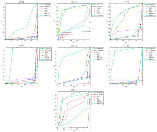
Figure 14.
The ROC curves of seven sequences.
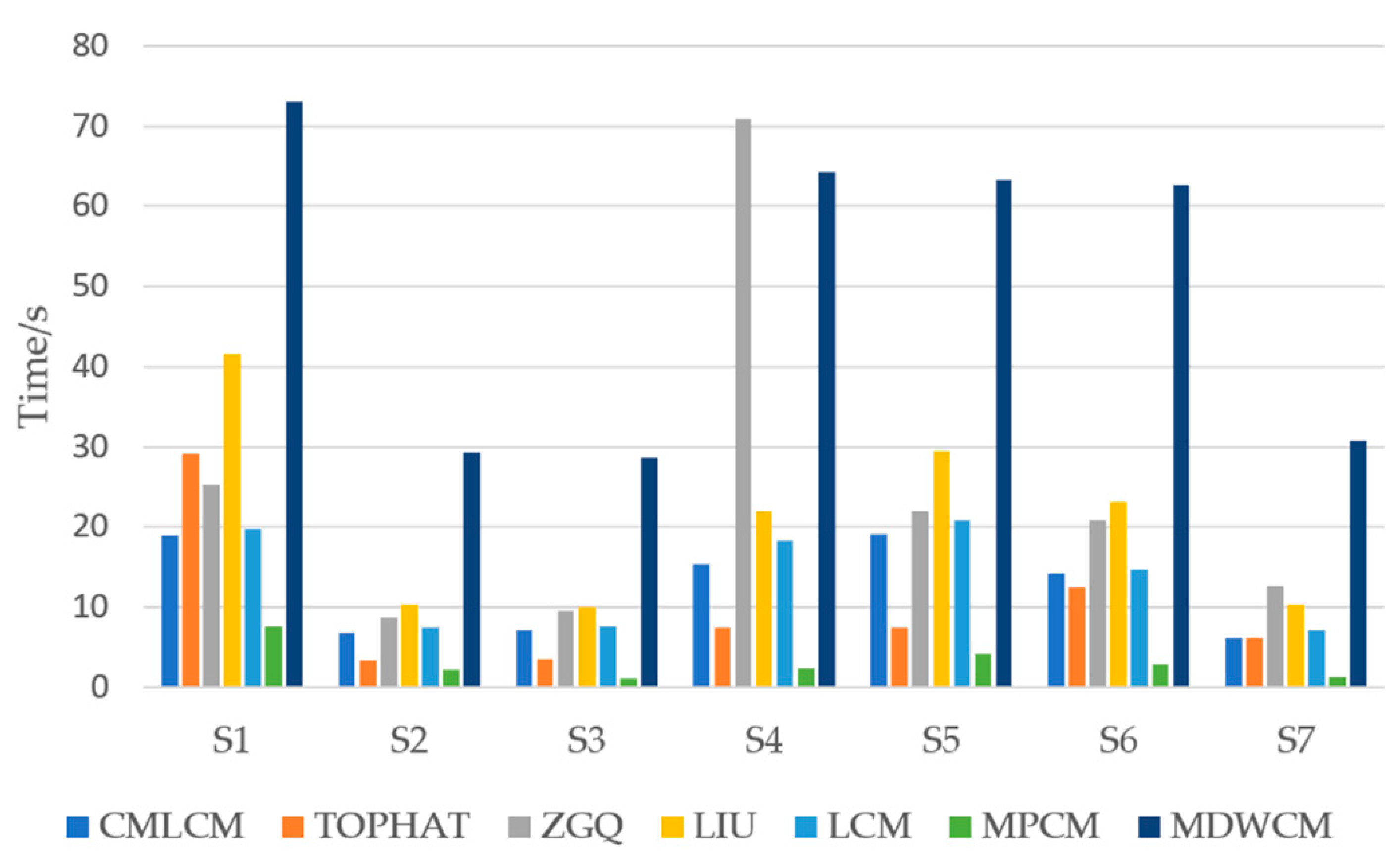
3.2.4. Time Consumption
Figure 15 shows a time consumption comparison among the different algorithms. The calculation time of the algorithm was the statistics from the step of image input to the step of threshold segmentation. As shown, the CMLCM algorithm proposed in this paper required less time than most algorithms, while it was more time-consuming than MPCM. Furthermore, based on the characteristics of the FPGA implementation platform, the idea of parallelization and pipeline combination [22] can be adopted to simultaneously calculate the second-order derivatives of multiple directions in FPGA. When the second-order derivatives are calculated, the threshold of the previous frame can be used to carry out segmentation of the image in this frame. This reduces the actual operation time greatly and the star image does not need to be scanned twice. Therefore, the CMLCM algorithm has high practicability in engineering.

Figure 15.
The time consumption of seven sequences for different algorithms.
4. Discussion
The experimental results indicated that the proposed CMLCM algorithm was not sensitive to noise. Besides, compared with other algorithms, the CMLCM algorithm had better star-extraction ability in complex backgrounds. At the same time, it had a higher detection rate under the same false alarm rate than the other algorithms. Moreover, the processing time of the algorithm was not high, and the overall architecture and calculation process of the algorithm made it very suitable for the transplantation in an embedded platform, which was of great help to actual on-orbit engineering. From the experimental results, it can be seen that the CMLCM algorithm has strong extraction ability with the interference of stray light, which can bring a great help to the performance of star sensor on orbit.
5. Conclusions
Considering the difficulty of star extraction with the interference of complex backgrounds, this paper proposes the CMLCM algorithm. The algorithm uses the second-order derivative characteristics of the star and background in four directions to enhance the star point and greatly suppress the complex background. Besides, it extracts the position of the star point by local threshold segmentation. The experimental results indicated that the CMLCM algorithm has high reliability and stability with the interference of stray light.
In the future, the CMLCM algorithm will be applied to an on-orbit task for further verification and to improve the capability of resisting disturbance in the star sensor.
Author Contributions
Conceptualization, E.L. and K.L.; methodology, K.L.; software, K.L.; validation, K.L. and H.Z.; formal analysis, H.T.; investigation, K.L.; resources, L.L. and R.Z.; data curation, K.L.; writing—original draft preparation, K.L.; writing—review and editing, R.Z.; visualization, K.L.; supervision, E.L.; project administration, K.L.; funding acquisition, R.Z. All authors have read and agreed to the published version of the manuscript.
Funding
This research was funded by the National Key Research and Development Program of China under Grant No. 2019YFA0706001.
Institutional Review Board Statement
Not applicable.
Informed Consent Statement
Not applicable.
Data Availability Statement
Not applicable.
Acknowledgments
This research was supported by the West Light Project of the Chinese Academy of Sciences. This research was also supported by the Special Talents Project of Organization Department of Sichuan Provincial Party Committee, and Science and Technology Talents Project of Sichuan Outstanding Youth.
Conflicts of Interest
The authors declare no conflict of interest.
References
- Liebe, C.C. Accuracy performance of star trackers—A tutorial. IEEE Trans. Aerosp. Electron. Syst. 2002, 38, 587–599. [Google Scholar] [CrossRef]
- Roger, J.C.; Santer, R.; Herman, M.; Deuzé, J.L. Polarization of the solar light scattered by the earth-atmosphere system as observed from the U.S. shuttle. Remote Sens. Environ. 1994, 48, 275–290. [Google Scholar] [CrossRef]
- Kwang-Yul, K.; Yoan, S. A Distance Boundary with Virtual Nodes for the Weighted Centroid Localization Algorithm. Sensors. 2018, 18, 1054. [Google Scholar] [CrossRef] [Green Version]
- Luo, L.Y.; Xu, L.P.; Zhang, H. Improved centroid extraction algorithm for autonomous star sensor. IET Image Process. 2015, 9, 901–907. [Google Scholar] [CrossRef]
- Fialho, M.; Mortari, D. Theoretical Limits of Star Sensor Accuracy. Sensors 2019, 19, 5355. [Google Scholar] [CrossRef] [PubMed] [Green Version]
- Seyed, M.F.; Reza, M.M.; Mahdi, N. Flying small target detection in ir images based on adaptive toggle operator. IET Comput. Vis. 2018, 12, 527–534. [Google Scholar] [CrossRef]
- Pillai, A.; Rajkumar, S.; Marimuthu, K.; Rajasekaran, G. Adaptive new top-hat transform and multi-scale sequential toggle operator based infrared image enhancement. In Proceedings of the 2017 Innovations in Power and Advanced Computing Technologies (i-PACT), Vellore, India, 21–22 April 2017; pp. 1–5. [Google Scholar] [CrossRef]
- Zhang, Y.; Du, B.; Zhang, L. A spatial filter based framework for target detection in hyperspectral imagery. In Proceedings of the 2013 5th Workshop on Hyperspectral Image and Signal Processing: Evolution in Remote Sensing (WHISPERS), Gainesville, FL, USA, 26–28 June 2013; pp. 1–4. [Google Scholar] [CrossRef]
- Wang, H.T.; Luo, C.Z.; Wang, Y.; Wang, X.Z.; Zhao, S.F. Algorithm for star extraction based on self-adaptive background prediction. Opt. Tech. 2009, 35, 412–414. [Google Scholar] [CrossRef]
- Yu, L.W.; Mao, X.N.; Jin, H.; Hu, X.C.; Wu, Y.K. Study on Image Process Method of Star Tracker for Stray Lights Resistance Filtering Based on Background. Aerosp. Shanghai 2016, 33, 26–31. [Google Scholar] [CrossRef]
- Liu, X.X.; Li, B.M.; Su, Q.T.; Liu, Z.H.; Wang, Y.L.; Yang, F. New exact labeling algorithm of connected regions in binary images. Comput. Eng. Appl. 2007, 43, 76–78. [Google Scholar] [CrossRef]
- Wang, X.Y.; Peng, Z.M.; Kong, D.H.; Zhang, H.; He, Y.M. Infrared dim target detection based on total variation regularization and principal component pursuit. Image Vis. Comput. 2017, 63, 1–9. [Google Scholar] [CrossRef]
- Zhao, Y.; Pan, H.; Du, C.; Zheng, Y. Principal curvature for infrared small target detection. Infrared Phys. Technol. 2015, 69, 36–43. [Google Scholar] [CrossRef]
- Zhu, G.Q.; Meng, X.Y.; Qian, W.X. Infrared Small Target Detection Method Based on Curvature near the Ground. Acta Photonica Sin. 2018, 47, 1010001. [Google Scholar] [CrossRef]
- Nasiri, M.; Mosavi, M.; Mirzakuchaki, S. Infrared Small Target Detection based on Human Visual Attention using Pulsed Discrete Cosine Transform. IET Image Processing 2017, 11, 397–405. [Google Scholar] [CrossRef]
- Chen, C.; Li, H.; Wei, Y.; Xia, T.; Tang, Y.Y. A local contrast method for small infrared target detection. IEEE Trans. Geosci. Remote Sens. 2014, 52, 574–581. [Google Scholar] [CrossRef]
- Han, J.; Ma, Y.; Zhou, B.; Fan, F.; Liang, K.; Fang, Y. A Robust Infrared Small Target Detection Algorithm Based on Human Visual System. Geoscience and Remote Sensing Letters. IEEE Geosci. Remote Sens. Lett. 2014, 11, 2168–2172. [Google Scholar] [CrossRef]
- Wei, Y.; You, X.; Li, H. Multiscale patch-based contrast measure for small infrared target detection. Pattern Recognit. 2016, 58, 216–226. [Google Scholar] [CrossRef]
- Lu, R.T.; Yang, X.G.; Li, W.P.; Ji, W.F.; Li, D.L.; Jing, X. Robust infrared small target detection via multidirectional derivative-based weighted contrast measure. IEEE Geosci. Remote Sens. Lett. 2020, 1, 1–5. [Google Scholar] [CrossRef]
- Haralick, R.M. Digital step edges from zero crossing of second directional derivatives. IEEE Trans. Pattern Anal. Mach. Intell. 1984, PAMI-6, 58–68. [Google Scholar] [CrossRef] [PubMed]
- Wang, H.; Xin, Y. Wavelet-based contourlet transform and kurtosis map for infrared small target detection in complex background. Sensors 2020, 20, 755. [Google Scholar] [CrossRef] [PubMed] [Green Version]
- Wang, X.; Wei, X.; Fan, Q.; Li, J.; Wang, G. Hardware implementation of fast and robust star centroid extraction with low resource cost. IEEE Sens. J. 2015, 15, 4857–4865. [Google Scholar] [CrossRef]
Publisher’s Note: MDPI stays neutral with regard to jurisdictional claims in published maps and institutional affiliations. |
© 2021 by the authors. Licensee MDPI, Basel, Switzerland. This article is an open access article distributed under the terms and conditions of the Creative Commons Attribution (CC BY) license (https://creativecommons.org/licenses/by/4.0/).


