Sequential Deep Learning with Feature Compression and Optimal State Estimation for Indoor Visible Light Positioning

Abstract

Visible Light Positioning (VLP) is widely regarded as a promising technology for high-precision indoor localization due to its immunity to radio-frequency interference and compatibility with existing Light-Emitting Diode (LED) lighting infrastructure. Despite recent progress, current VLP systems remain fundamentally limited by nonlinear received signal strength (RSS) characteristics, unknown transmitter orientations, and dynamic indoor disturbances. Existing solutions typically address these challenges in isolation, resulting in limited robustness and scalability. This paper proposes SCENE-VLP (Sequential Deep Learning with Feature Compression and Optimal State Estimation), a structured positioning framework that integrates feature compression, temporal sequence modeling, and probabilistic state refinement within a unified estimation pipeline. Specifically, SCENE-VLP combines Principal Component Analysis (PCA) and Denoising Autoencoders (DAE) for linear and nonlinear observation conditioning, Gated Recurrent Units (GRU) for modeling temporal dependencies in RSS sequences, and Kalman-based filtering (KF/EKF) for recursive state-space refinement. The framework is formulated as a hierarchical approximation of the nonlinear observation model, linking data-driven measurement learning with Bayesian state estimation. A systematic ablation study across multiple scenarios, including same-dataset evaluation and cross-dataset generalization, demonstrates that each component provides complementary benefits. Feature compression reduces redundancy while preserving dominant signal structure; GRU significantly improves robustness over static regression; and recursive filtering consistently reduces positioning error compared to unfiltered predictions. While both KF and EKF improve performance, EKF provides incremental refinement under mild nonlinearities. Extensive simulations conducted on an indoor dataset collected from a realistic deployment with eight ceiling-mounted LEDs and a single photodetector (PD) show that SCENE-VLP achieves sub-decimeter localization accuracy, with P50 and P95 errors of 1.84 cm and 6.52 cm, respectively. Cross-scenario evaluation further confirms stable generalization and statistically consistent improvements. These results demonstrate that the structured integration of observation conditioning, temporal modeling, and Bayesian refinement yields measurable gains beyond partial pipeline configurations, establishing SCENE-VLP as a robust and scalable solution for next-generation indoor visible light positioning systems.

1. Introduction

The rapid development of smart mobile devices, the Internet of Things (IoT), and artificial intelligence (AI) has significantly expanded the use of indoor location-aware services. Applications such as smart manufacturing, warehouse automation, healthcare monitoring, augmented reality (AR), and intelligent transportation increasingly rely on accurate and reliable indoor positioning [1]. These emerging applications demand localization systems capable of providing high precision, low latency, and robust performance in complex indoor environments. Although the Global Positioning System (GPS) has become the dominant technology for outdoor positioning, its performance indoors is severely limited. GPS signals experience strong attenuation when penetrating building structures and are highly susceptible to multipath and shadowing effects, resulting in poor positioning accuracy and unreliable coverage [2]. Consequently, various alternative indoor positioning technologies have been investigated, including wireless local area networks (WLAN), Bluetooth, ZigBee, and ultra-wideband (UWB). While these radio-frequency (RF)-based solutions have shown promising results, they often suffer from electromagnetic interference, spectrum congestion, and the need for additional infrastructure, which can increase deployment cost and limit scalability [3]. Optical wireless communication (OWC) has emerged as a compelling alternative for short-range wireless systems by exploiting the visible light spectrum. Visible Light Communication (VLC), which uses light-emitting diodes (LEDs) for simultaneous illumination and communication, has attracted considerable attention as a key enabling technology for future wireless networks [4]. Building on VLC, Visible Light Positioning (VLP) has become a promising solution for indoor localization due to its high positioning accuracy, immunity to electromagnetic interference, and ability to reuse existing lighting infrastructure [5]. These characteristics make VLP particularly attractive for applications requiring precise and reliable indoor positioning.

Recent studies have demonstrated that VLP systems can achieve centimeter-level accuracy under controlled conditions, although practical deployment still faces several challenges [6]. The increasing demand for precise indoor positioning in emerging applications has further stimulated research efforts in this area. However, real-world indoor environments introduce various impairments, including multipath reflections, non-line-of-sight propagation, signal attenuation, and shadowing, all of which significantly affect positioning performance. Existing VLP approaches can generally be categorized into model-based and data-driven methods. Model-based techniques, such as received signal strength (RSS), angle of arrival (AoA), and time-based methods, rely on analytical channel models to estimate positions [7]. Although these techniques are effective under ideal assumptions, their accuracy is often degraded in practical environments due to mismatches between theoretical models and real-world propagation conditions. Variations in LED radiation patterns, reflections from surfaces, and environmental dynamics further complicate accurate channel modeling [8]. To overcome these limitations, model-free approaches such as fingerprinting and proximity-based localization have been investigated. Fingerprinting methods use empirical signal measurements to estimate positions, improving robustness against modeling inaccuracies [9]. However, maintaining accurate and up-to-date fingerprint databases is challenging in dynamic indoor environments where lighting conditions and obstacles frequently change. Proximity-based techniques, while simpler to implement, generally provide lower positioning accuracy and remain sensitive to environmental variations [4].

In recent years, machine learning (ML) techniques have been increasingly integrated into VLP systems to enhance localization accuracy and robustness [10]. By learning complex nonlinear relationships between signal features and spatial coordinates, ML-based approaches can effectively handle noise, multipath effects, and environmental uncertainties [11]. Despite these advances, achieving reliable and stable positioning in dynamic indoor environments remains a challenging task, particularly when temporal variations and measurement noise are present. Motivated by these challenges, this work investigates a robust data-driven framework for indoor visible light positioning that aims to improve positioning accuracy and stability under realistic indoor conditions. The proposed approach focuses on enhancing signal representation, mitigating noise and environmental variations, and improving temporal consistency in position estimation. The details of the related work and the methodology are presented in the subsequent sections.

2. Related Work

A variety of techniques have been proposed for indoor VLP, ranging from analytical estimation methods to data-driven machine learning approaches. Early VLP systems primarily relied on geometric and optimization-based techniques to estimate the receiver position. A range of methods has been explored for estimating the position of a receiver in RSS-based VLP systems. Among these, analytical approaches based on least-squares optimization are frequently adopted because of their low computational complexity and straightforward implementation [12]. For instance, both linear least squares (LLS) and nonlinear least squares (NLLS) algorithms have been employed for position estimation, where reported experimental results indicate that NLLS achieves a lower minimum positioning error of approximately 46.42 cm compared to about 55.89 cm obtained with LLS [5]. Despite this improvement, least-squares-based techniques remain sensitive to measurement noise, multipath reflections, and inaccuracies in channel modeling, which can significantly degrade localization performance in practical indoor environments [5]. To further improve positioning accuracy, hybrid geometric and optimization-based techniques have also been proposed. In [13], an efficient RSS-based VLP algorithm was developed to estimate the three-dimensional location of a receiver by combining two-dimensional trilateration with nonlinear least-squares refinement. The proposed approach improved estimation stability and accuracy compared to conventional methods, demonstrating the effectiveness of combining geometric positioning with optimization techniques. Nevertheless, such approaches still rely heavily on accurate channel modeling and are susceptible to environmental dynamics, reflections, and shadowing, which are difficult to model precisely in practical indoor scenarios. These limitations of model-based approaches have motivated the growing adoption of data-driven and machine learning techniques for indoor VLP.

Machine learning methods are capable of capturing complex nonlinear relationships between signal features and spatial coordinates, making them particularly suitable for indoor localization problems where analytical channel modeling becomes impractical. Raes et al. showed that a multilayer perceptron (MLP) and a Gaussian process model can outperform traditional RSS multilateration under varying signal conditions [14]. Neural networks can naturally accommodate complex nonlinear relationships in the data that challenge analytical models [14], making them well suited to the learning aspects required in indoor VLP. Yang et al. [15] proposed a three-dimensional indoor VLP system based on a GRU neural network, employing two ceiling-mounted LEDs and three hemispherical photodetectors (PD). They incorporated a learning rate attenuation strategy to stabilize GRU training and achieved centimeter-level mean errors (≈2.66–2.69 cm). Their approach, however, processes high-dimensional raw RSS fingerprints without feature compression or dimensionality reduction, which increases model complexity. Moreover, no temporal filtering or robustness evaluation was performed to address higher-order propagation effects. Gufran et al. [16] presented SANGRIA, a stacked autoencoder-based framework that compresses high-dimensional RSS features before applying a gradient-boosted trees regressor. This feature compression step improved generalization and helped to address device heterogeneity, enabling SANGRIA to outperform several state-of-the-art methods (over 42% lower localization error on average) across diverse indoor environments [16]. However, SANGRIA operates in a static setting and treats localization as a one-shot regression problem. Without sequential modeling or online filtering, it cannot leverage temporal continuity or smooth measurement fluctuations, limiting its suitability for real-time user tracking.

Hybrid learning and filtering approaches have also been investigated to improve positioning stability. Tian et al. [17] introduced a hybrid long short-term memory (LSTM) network combined with a Kalman filter (KF-LSTM) for indoor ultra-wideband (UWB) positioning. The temporal filtering improved prediction stability and positioning accuracy and achieved over 49% lower mean error compared to using an LSTM alone. However, the method is designed specifically for UWB radio signals and assumes primarily Gaussian noise. It does not account for the unique optical channel characteristics of VLP, such as Lambertian propagation and sensitivity to ambient illumination, making direct transfer from UWB to VLP non-trivial. Similarly, Mao et al. [18] developed a VLP system combining a deep neural network (DNN), cluster optimization, and Kalman filtering. Clustering reduces training complexity, while Kalman filtering stabilizes trajectory estimation. However, the lack of a feature compression stage and the use of a feedforward DNN limit the system’s ability to model sequential dependencies in dynamic indoor scenarios. Recent studies have also explored machine learning techniques for optimizing VLC and VLP system performance under practical constraints, including channel variations and energy efficiency, further highlighting the growing role of intelligent data-driven approaches in optical wireless systems [7,11].

In summary, previous works either model temporal dependencies without addressing high-dimensional RSS features [15], or apply feature compression without leveraging sequential or filtering mechanisms [16]. Hybrid filtering approaches designed for RF-based positioning [17] are not optimized for optical channel characteristics. Furthermore, conventional geometric and least-squares-based approaches remain sensitive to channel modeling inaccuracies and environmental dynamics. To date, no VLP framework jointly integrates feature compression, sequential modeling, and probabilistic state estimation within a unified architecture. Therefore, this work introduces SCENE-VLP, a comprehensive solution that unifies these components for robust indoor localization.

The paper follows this structure: Section 3 introduces the system model, and Section 4 presents results and discussions. Finally, Section 5 summarizes our contributions and concludes the work.

3. System Model

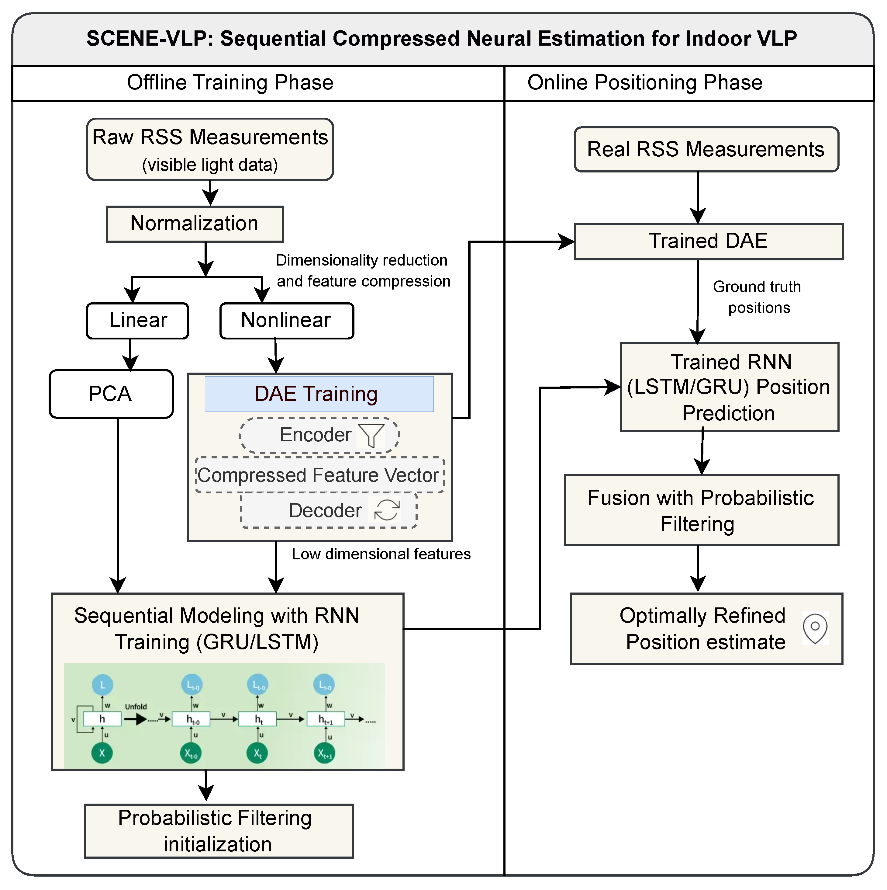
As illustrated in Figure 1, SCENE-VLP operates in two stages: an offline training phase and an online localization phase. In the offline phase, a dataset of RSS measurements (e.g., from PD sensors observing LED beacons) along with ground-truth positions is collected. The overall pipeline is organized into three main blocks: feature compression, recurrent position estimation, and Kalman-based probabilistic refinement, which are consistently applied across both phases. The RSS data are first normalized to a common scale to improve neural network convergence. Feature extraction is then performed using either PCA for linear dimensionality reduction [19] or a DAE for nonlinear noise suppression and compact latent representation learning [20], enabling a controlled comparison between linear and nonlinear compression strategies within the same downstream GRU–EKF estimator. These lower-dimensional features are fed into a recurrent neural network, such as a GRU or LSTM, which learns to map temporal RSS sequences to 2D position estimates [21], with GRU adopted as the primary backbone due to its favorable trade-off between modeling capacity and computational cost. During the online phase, incoming RSS measurements are processed using the same feature encoder (PCA or DAE). For the DAE, only the encoder is used at inference time, while the decoder is employed exclusively during offline training. The encoded features are passed through the trained recurrent network to produce position predictions. To ensure temporal smoothness and physical consistency, these predictions are further refined using probabilistic filters, specifically the KF and EKF, which fuse the data-driven RNN output with a motion model [22]. The KF is suitable for near-linear, Gaussian dynamics, whereas the EKF accommodates nonlinear behavior typical of indoor optical channels. Importantly, the SCENE-VLP architecture is not a simple concatenation of independent processing blocks, but a structured estimation pipeline in which each module fulfills a distinct algorithmic role. From a state-space estimation perspective, SCENE-VLP can be interpreted as a structured approximation of an unknown nonlinear observation model. Classical VLP systems rely on analytical channel models to define the measurement function $\mathbf{h}\left({\mathbf{x}}_t\right)$. In contrast, the GRU in SCENE-VLP implicitly learns a data-driven approximation of this mapping from compressed RSS sequences to position estimates. The feature compression stage reduces observation redundancy and stabilizes the covariance structure of the RSS input, thereby improving the conditioning of the learned measurement function. The GRU reduces short-term conditional measurement variance by incorporating temporal context into the learned observation function, while the EKF performs Bayesian posterior correction by enforcing a Markovian state transition model and propagating uncertainty through ${\mathbf{P}}_{t|t}$. Thus, the integration represents a hierarchical refinement of the measurement-to-state mapping rather than empirical module stacking. The following subsections detail each component of the SCENE-VLP system model, including the optical channel formulation, feature extraction pipeline, sequential learning architecture, and the Kalman-based filtering framework.

3.1. Communication Model

In this work, we consider an indoor environment where L LEDs serve as transmitters, positioned at a height $h_{\mathrm{LED}}$ above the observation plane of a photodiode (PD) receiver. Each LED, indexed by $k=1,\dots ,L$, emits an intensity-modulated optical waveform characterized by a distinct fundamental frequency $f_k$. This frequency-division multiplexing enables the receiver to differentiate and isolate signals from individual LEDs. The intensity-modulated waveform transmitted by LED k is given by [23]:

$$\begin{array}{c}\hfill s_k\left(t\right)={\displaystyle \frac{P_{\mathrm{tx}}}{2}}\left[1+sgn\left(sin(2\pi f_{k}t+{\psi }_k)\right)\right],\end{array}$$

(1)

where $P_{\mathrm{tx}}$ is the peak optical power, $f_k$ is the unique modulation frequency, and ${\psi }_k$ is a random initial phase offset for LED k. The PD receiver captures the aggregate of these optical signals and converts them into a composite electrical signal $v_{\mathrm{rx}}\left(t\right)$:

$$\begin{array}{c}\hfill v_{\mathrm{rx}}\left(t\right)=\sum _{k=1}^L{g}_k\mathcal{R}{s}_k\left(t\right)+I_{\mathrm{amb}}+{\eta }_{\mathrm{rx}}\left(t\right),\end{array}$$

(2)

where $\mathcal{R}$ is the PD responsivity, $g_k$ is the optical channel gain between LED k and the PD, $I_{\mathrm{amb}}$ is the DC contribution from ambient light, and ${\eta }_{\mathrm{rx}}\left(t\right)$ is an additive noise term. The gain $g_k$ depends on geometric and photometric properties:

$$\begin{array}{c}\hfill g_k=\mathcal{F}(d_k,A_{\mathrm{PD}},{\theta }_k,{\iota }_k),\end{array}$$

(3)

where $d_k$ is the LED–PD distance, $A_{\mathrm{PD}}$ is the PD effective area, ${\theta }_k$ is the irradiance angle, and ${\iota }_k$ is the incidence angle [15]. To emulate practical operating conditions, the additive noise ${\eta }_{\mathrm{rx}}\left(t\right)$ in (2) is modeled as a zero-mean Gaussian random variable with variance ${\sigma }^2$ [24]:

$$\begin{array}{c}\hfill {\eta }_{\mathrm{rx}}\left(t\right)\sim \mathcal{N}(0,{\sigma }^2),\end{array}$$

(4)

where ${\sigma }^2$ represents the noise power, which accounts for sensor imperfections, electronic interference, and fluctuations in ambient light. At each time t, the demodulation process extracts the RSS contribution from each LED. These contributions are arranged into an L-dimensional vector:

$$\begin{array}{c}\hfill {\mathbf{r}}_t={\left[r_1\left(t\right),r_2\left(t\right),\dots ,r_L\left(t\right)\right]}^{\top },\end{array}$$

(5)

where $r_k\left(t\right)$ denotes the instantaneous RSS from LED k at time t, and ${\mathbf{r}}_t\in {\mathbb{R}}^L$ compactly captures the multi-channel RSS information from all L transmitters at that instant. This vector serves as the high-dimensional input feature for the localization system. In the SCENE-VLP framework, the PCA or DAE encoder first processes ${\mathbf{r}}_t$, whose encoded output is then passed through the RNN models, and finally refined using a Kalman or Extended Kalman filtering to yield accurate and stable position estimates.

3.2. Feature Compression with PCA and DAE

To mitigate the impact of noise and reduce feature dimensionality, SCENE-VLP incorporates a feature compression step before the RNN. Prior to feature compression, the RSS measurements are normalized to ensure numerical stability and to prevent features with larger magnitudes from dominating the learning process. Specifically, a z-score normalization (standardization) is applied to each RSS feature independently, such that the resulting features have zero mean and unit variance. Let ${\mathbf{r}}_t\in {\mathbb{R}}^L$ denote the raw RSS vector at time instant t, where L is the number of RSS features. The normalized RSS vector ${\tilde{\mathbf{r}}}_t$ is computed as

$${\tilde{\mathbf{r}}}_t={\displaystyle \frac{{\mathbf{r}}_t-\mu }{\sigma }},$$

(6)

where $\mu$ and $\sigma$ denote the feature-wise mean and standard deviation computed from the training dataset, respectively. The same normalization parameters are subsequently applied to the validation and test sets to avoid data leakage. After normalization, we explore both a linear PCA method and a non-linear DAE method to transform the normalized RSS vectors into a lower-dimensional representation that preserves essential information while filtering out noise. Throughout this section, bold symbols denote vectors, and a tilde $\left(\widetilde{·}\right)$ indicates normalized RSS quantities. For clarity, we denote each normalized RSS input vector as ${\tilde{\mathbf{r}}}_t\in {\mathbb{R}}^L$, its PCA-compressed representation as ${\mathbf{z}}_t^{\mathrm{PCA}}$, and its DAE-encoded latent representation as ${\mathbf{z}}_t^{\mathrm{DAE}}$.

3.2.1. PCA

Let $\tilde{\mathbf{R}}\in {\mathbb{R}}^{N\times L}$ denote the normalized RSS data matrix, where N is the number of samples and L is the number of RSS features, assuming $L<N$ so that the sample covariance matrix is well-conditioned. Since the RSS features are standardized to zero mean, the sample covariance matrix $\mathbf{C}$ can be computed as

$$\begin{array}{c}\hfill \mathbf{C}={\displaystyle \frac{1}{N-1}}{\tilde{\mathbf{R}}}^{\top }\tilde{\mathbf{R}}.\end{array}$$

(7)

PCA proceeds by solving the eigenvalue problem

$$\begin{array}{c}\hfill \mathbf{C}{\mathbf{u}}_i={\lambda }_i{\mathbf{u}}_i,\end{array}$$

(8)

where ${\lambda }_i$ are the eigenvalues and ${\mathbf{u}}_i$ are the corresponding eigenvectors.

Since the covariance matrix $\mathbf{C}$ is symmetric and positive semi-definite, all eigenvalues satisfy ${\lambda }_i\ge 0$. The eigenvalues are sorted in descending order,

$${\lambda }_1\ge {\lambda }_2\ge \dots \ge {\lambda }_L\ge 0,$$

and the first k eigenvectors are selected to construct the PCA projection matrix

$$\mathbf{W}=\left[{\mathbf{u}}_1,{\mathbf{u}}_2,\dots ,{\mathbf{u}}_k\right]\in {\mathbb{R}}^{L\times k}.$$

Each normalized RSS vector ${\tilde{\mathbf{r}}}_t\in {\mathbb{R}}^L$ is then projected into the k-dimensional PCA subspace as

$$\begin{array}{c}\hfill {\mathbf{z}}_t^{\mathrm{PCA}}={\mathbf{W}}^{\top }{\tilde{\mathbf{r}}}_t,\end{array}$$

(9)

where ${\mathbf{z}}_t^{\mathrm{PCA}}\in {\mathbb{R}}^k$ denotes the reduced feature vector that preserves the dominant variance of the original RSS measurements.

3.2.2. DAE

In SCENE-VLP, the DAE performs nonlinear feature compression and enhances robustness against noise. For each normalized RSS input ${\tilde{\mathbf{r}}}_t\in {\mathbb{R}}^L$, the encoder maps the high-dimensional observation to a compressed latent representation ${\mathbf{z}}_t^{\mathrm{DAE}}\in {\mathbb{R}}^k$ as

$$\begin{array}{c}\hfill {\mathbf{z}}_t^{\mathrm{DAE}}=\varphi \left({\mathbf{W}}_e{\tilde{\mathbf{r}}}_t+{\mathbf{b}}_e\right),\end{array}$$

(10)

where ${\mathbf{W}}_e$ and ${\mathbf{b}}_e$ denote the encoder weight matrix and bias vector, and $\varphi (·)$ is a nonlinear activation function implemented using ReLU. The decoder reconstructs the input as

$$\begin{array}{c}\hfill {\widehat{\mathbf{r}}}_t=\psi \left({\mathbf{W}}_d{\mathbf{z}}_t^{\mathrm{DAE}}+{\mathbf{b}}_d\right),\end{array}$$

(11)

with ${\mathbf{W}}_d$ and ${\mathbf{b}}_d$ denoting the decoder parameters and $\psi (·)$ the decoder activation.

The DAE is trained by minimizing the mean squared error (MSE) between the original normalized RSS vector ${\tilde{\mathbf{r}}}_t$ and its reconstruction ${\widehat{\mathbf{r}}}_t$:

$$\begin{array}{c}\hfill {\mathcal{L}}_{\mathrm{DAE}}={\displaystyle \frac{1}{N}}\sum _{t=1}^N\parallel {\tilde{\mathbf{r}}}_t-{\widehat{\mathbf{r}}}_t{\parallel }^2.\end{array}$$

(12)

In the denoising setup, the autoencoder receives a corrupted version ${\tilde{\mathbf{r}}}_t^{\prime }$ as input, while being trained to reconstruct the clean signal ${\tilde{\mathbf{r}}}_t$. This encourages the encoder to extract latent features that preserve the essential structure of the RSS patterns while suppressing noise, multipath distortion, and device-level variations. Once trained offline, only the encoder is retained during the online phase of SCENE-VLP. Each incoming RSS vector is passed through the encoder to produce ${\mathbf{z}}_t^{\mathrm{DAE}}$, which serves as the input feature vector to the RNN model.

3.3. Recurrent Neural Network Modeling

The SCENE-VLP framework employs an RNN to model the temporal evolution of compressed RSS features. At each time step t, the network processes a compressed input vector ${\mathbf{z}}_t$ representing either ${\mathbf{z}}_t^{\mathrm{PCA}}$ or ${\mathbf{z}}_t^{\mathrm{DAE}}$ and updates its hidden state ${\mathbf{h}}_t$, which summarizes past inputs and provides temporal context for position estimation. Gated architectures such as GRUs and LSTMs extend the simple RNN by introducing gating mechanisms that mitigate vanishing gradients and enable stable learning over long sequences [15]. A generic gated recurrent update can be expressed as:

$$\begin{array}{cc}\hfill {\mathbf{g}}_t& =\sigma \left({\mathbf{W}}_g{\mathbf{z}}_t+{\mathbf{U}}_g{\mathbf{h}}_{t-1}+{\mathbf{b}}_g\right),\hfill \end{array}$$

(13)

$$\begin{array}{cc}\hfill {\tilde{\mathbf{c}}}_t& =tanh\left({\mathbf{W}}_c{\mathbf{z}}_t+{\mathbf{U}}_c{\mathbf{h}}_{t-1}+{\mathbf{b}}_c\right),\hfill \end{array}$$

(14)

$$\begin{array}{cc}\hfill {\mathbf{c}}_t& =F({\mathbf{c}}_{t-1},{\mathbf{g}}_t,{\tilde{\mathbf{c}}}_t),\hfill \end{array}$$

(15)

$$\begin{array}{cc}\hfill {\mathbf{h}}_t& =O({\mathbf{c}}_t,{\mathbf{g}}_t),\hfill \end{array}$$

(16)

where ${\mathbf{z}}_t$ is the compressed feature vector, ${\mathbf{h}}_t$ the hidden state, ${\mathbf{c}}_t$ the memory state, ${\mathbf{g}}_t$ a gating vector, and $\mathbf{W}$, $\mathbf{U}$, and $\mathbf{b}$ are trainable parameters. In the GRU architecture, the hidden state update is given by

$$\begin{array}{c}\hfill {\mathbf{h}}_t=(1-{\mathbf{u}}_t)\odot {\mathbf{h}}_{t-1}+{\mathbf{u}}_t\odot {\tilde{\mathbf{h}}}_t,\end{array}$$

(17)

where ${\mathbf{u}}_t$ is the update gate and ⊙ denotes element-wise (Hadamard) multiplication. The candidate’s hidden state is computed as

$$\begin{array}{c}\hfill {\tilde{\mathbf{h}}}_t=tanh\left({\mathbf{W}}_h{\mathbf{z}}_t+{\mathbf{U}}_h\left({\mathbf{r}}_t^{\mathrm{reset}}\odot {\mathbf{h}}_{t-1}\right)+{\mathbf{b}}_h\right),\end{array}$$

(18)

where ${\mathbf{r}}_t^{\mathrm{reset}}$ denotes the reset gate defined as

$$\begin{array}{c}\hfill {\mathbf{r}}_t^{\mathrm{reset}}=\sigma \left({\mathbf{W}}_r{\mathbf{z}}_t+{\mathbf{U}}_r{\mathbf{h}}_{t-1}+{\mathbf{b}}_r\right).\end{array}$$

(19)

The network outputs a position estimate

$$\begin{array}{c}\hfill {\tilde{\mathbf{p}}}_t=f_{\mathrm{RNN}}\left({\mathbf{z}}_{1:t}\right),\end{array}$$

(20)

where ${\tilde{\mathbf{p}}}_t={[{\widehat{x}}_t,{\widehat{y}}_t]}^{\top }\in {\mathbb{R}}^2$ represents the predicted receiver location at time t. The probabilistic filtering stage subsequently refines these sequential predictions.

3.4. Probabilistic Filtering

To refine the RNN-based position estimates, SCENE-VLP employs probabilistic filtering using either the KF or its nonlinear extension, the EKF. Let ${\mathbf{x}}_t$ denote the system state (e.g., receiver position and optional velocity), and let the RNN output ${\tilde{\mathbf{p}}}_t$ serve as the measurement. In this work, ${\mathbf{x}}_t$ is taken as ${[x_t,y_t]}^{\top }$ for position-only tracking and can be extended to ${[x_t,y_t,{\dot{x}}_t,{\dot{y}}_t]}^{\top }$ when explicit velocity modeling is required for smoother motion continuity. The filtering model is

$$\begin{array}{cc}\hfill {\mathbf{x}}_t& =\mathbf{f}\left({\mathbf{x}}_{t-1}\right)+{\mathbf{w}}_t,\hfill \end{array}$$

(21)

$$\begin{array}{cc}\hfill {\mathbf{y}}_t& =\mathbf{h}\left({\mathbf{x}}_t\right)+{\mathbf{v}}_t,\hfill \end{array}$$

(22)

where ${\mathbf{y}}_t={\tilde{\mathbf{p}}}_t$, ${\mathbf{w}}_t\sim \mathcal{N}(\mathbf{0},\mathbf{Q})$ is the process noise with covariance $\mathbf{Q}$, and ${\mathbf{v}}_t\sim \mathcal{N}(\mathbf{0},\mathbf{R})$ is the measurement noise with covariance $\mathbf{R}$. The functions $\mathbf{f}(·)$ and $\mathbf{h}(·)$ represent the state transition model and the measurement model, respectively. In SCENE-VLP, the RNN output ${\tilde{\mathbf{p}}}_t$ is treated as a pseudo-measurement of the true receiver state. Following the standard Kalman measurement model, its measurement error is modeled as approximately unbiased (zero mean), i.e., $\mathbb{E}\left[{\mathbf{v}}_t\right]=\mathbf{0}$, with covariance $\mathbf{R}$. To validate this assumption, we compute the mean residual between ${\tilde{\mathbf{p}}}_t$ and the ground-truth positions on a held-out validation set. If a non-negligible bias is observed, the estimated residual mean is subtracted from ${\tilde{\mathbf{p}}}_t$ prior to the EKF update, so that the EKF operates under the standard zero-mean measurement noise assumption. Based on this state space model, the filtering procedure proceeds through the following two stages.

(i)

Prediction

$$\begin{array}{cc}\hfill {\widehat{\mathbf{x}}}_{t|t-1}& =\mathbf{f}\left({\widehat{\mathbf{x}}}_{t-1|t-1}\right),\hfill \end{array}$$

(23)

$$\begin{array}{cc}\hfill {\mathbf{P}}_{t|t-1}& ={\mathbf{F}}_t{\mathbf{P}}_{t-1|t-1}{\mathbf{F}}_t^{\top }+\mathbf{Q},\hfill \end{array}$$

(24)

where ${\widehat{\mathbf{x}}}_{t|t-1}$ is the predicted state, ${\mathbf{P}}_{t|t-1}$ the predicted covariance, and ${\mathbf{F}}_t$ is the Jacobian of $\mathbf{f}(·)$ evaluated at ${\widehat{\mathbf{x}}}_{t-1|t-1}$.

(ii)

Update

$$\begin{array}{cc}\hfill {\mathbf{K}}_t& ={\mathbf{P}}_{t|t-1}{\mathbf{H}}_t^{\top }{\left({\mathbf{H}}_t{\mathbf{P}}_{t|t-1}{\mathbf{H}}_t^{\top }+\mathbf{R}\right)}^{-1},\hfill \end{array}$$

(25)

$$\begin{array}{cc}\hfill {\widehat{\mathbf{x}}}_{t|t}& ={\widehat{\mathbf{x}}}_{t|t-1}+{\mathbf{K}}_t\left({\mathbf{y}}_t-\mathbf{h}\left({\widehat{\mathbf{x}}}_{t|t-1}\right)\right),\hfill \end{array}$$

(26)

$$\begin{array}{cc}\hfill {\mathbf{P}}_{t|t}& =(\mathbf{I}-{\mathbf{K}}_t{\mathbf{H}}_t){\mathbf{P}}_{t|t-1},\hfill \end{array}$$

(27)

where ${\mathbf{K}}_t$ is the Kalman gain, ${\mathbf{H}}_t$ is the Jacobian of $\mathbf{h}(·)$ evaluated at ${\widehat{\mathbf{x}}}_{t|t-1}$, and ${\mathbf{P}}_{t|t}$ is the updated state covariance.

The above equations describe the general EKF formulation. The classical KF appears as the linear special case when

$$\mathbf{f}\left(\mathbf{x}\right)=\mathbf{F}\mathbf{x},\mathbf{h}\left(\mathbf{x}\right)=\mathbf{H}\mathbf{x},$$

so that ${\mathbf{F}}_t=\mathbf{F}$ and ${\mathbf{H}}_t=\mathbf{H}$, eliminating the need for Jacobian computation. This formulation clarifies how SCENE-VLP employs KF where dynamics are linear and EKF where nonlinearities dominate.

3.5. Unified State-Space Formulation and Algorithmic Implementation

The mathematical formulation of the SCENE-VLP model presented in Section 3.2, Section 3.3 and Section 3.4 is summarized by

$$\begin{array}{c}{\widehat{\mathbf{x}}}_{t|t}={\widehat{\mathbf{x}}}_{t|t-1}+{\mathbf{K}}_t\left({\tilde{\mathbf{p}}}_t-{\mathbf{H}}_t{\widehat{\mathbf{x}}}_{t|t-1}\right)\end{array}$$

(28)

Equation (28) shows that ${\widehat{\mathbf{x}}}_{t|t-1}$ denotes the predicted state obtained from the motion model, ${\mathbf{K}}_t$ is the Kalman gain that balances prediction and measurement, and ${\tilde{\mathbf{p}}}_t=f_{\mathrm{GRU}}\left({\mathbf{z}}_{1:t}\right)$ represents the position estimate produced by the GRU from compressed RSS sequences. Here, $\mathbf{\Phi }(·)$ denotes the selected feature encoder (PCA or DAE) used in the corresponding SCENE-VLP configuration, where ${\mathbf{z}}_t=\mathbf{\Phi }\left({\tilde{\mathbf{r}}}_t\right)$ and ${\mathbf{z}}_{1:t}$ represents the sequence of compressed RSS inputs. The matrix ${\mathbf{H}}_t$ maps the predicted state to the observation space and is typically chosen as the identity matrix.

The refined receiver position is obtained from the positional components of the filtered state,

$${\widehat{\mathbf{p}}}_t=\left[\begin{array}{c}{\widehat{x}}_{t|t}\\ {\widehat{y}}_{t|t}\end{array}\right].$$

The complete recursive realization of (28) is implemented through the offline training phase described in Algorithm 1 and the online inference and EKF-based refinement detailed in Algorithm 2. These algorithms clarify that SCENE-VLP is not an empirical stacking of modules, but a structured estimator in which feature compression conditions the observation space, the GRU captures temporal dependencies, and the EKF enforces motion consistency and uncertainty-aware correction. The benefit of this integration is quantified through the experimental evaluation presented in Section 4.

Algorithm 1 SCENE-VLP Offline Training: Feature Compression and GRU Learning (Section 3.2 and Section 3.3)

Require: Training set $\mathcal{D}={\left\{({\mathbf{r}}_t,{\mathbf{p}}_t)\right\}}_{t=1}^N$, ${\mathbf{r}}_t\in {\mathbb{R}}^L$; encoder type $\mathsf{\Phi }\in \{\mathrm{PCA},\mathrm{DAE}\}$; latent dimension        k; sequence length T Ensure: Trained encoder $\mathsf{\Phi }(·)$ and GRU model $f_{\mathrm{GRU}}(·)$       1: Compute RSS normalization parameters $\mathsf{\Omega }=(\mathit{\mu },\mathit{\sigma })$       2: for $t=1$ to N do       3:       ${\tilde{\mathbf{r}}}_t\leftarrow \mathrm{Norm}({\mathbf{r}}_t;\mathsf{\Omega })$       4: end for       5: if $\mathsf{\Phi }$ is PCA then       6:       Compute covariance matrix and eigen-decomposition       7:       Select top-k eigenvectors and form projection matrix $\mathbf{W}$       8:       Define encoder $\mathsf{\Phi }\left(\tilde{\mathbf{r}}\right)={\mathbf{W}}^{\top }\tilde{\mathbf{r}}$       9: else     10:       Train denoising autoencoder by minimizing reconstruction error     11:       Retain encoder $\mathsf{\Phi }\left(\tilde{\mathbf{r}}\right)=\varphi ({\mathbf{W}}_e\tilde{\mathbf{r}}+{\mathbf{b}}_e)$     12: end if     13: for $t=1$ to N do     14:       ${\mathbf{z}}_t\leftarrow \mathsf{\Phi }\left({\tilde{\mathbf{r}}}_t\right)$     15: end for     16: Construct sequences ${\mathbf{Z}}_t=[{\mathbf{z}}_{t-T+1},\dots ,{\mathbf{z}}_t]$     17: Train GRU regressor $f_{\mathrm{GRU}}\left({\mathbf{Z}}_t\right)\to {\mathbf{p}}_t$

Algorithm 2 SCENE-VLP Online Inference: GRU-Based Estimation with EKF Refinement (Section 3.3 and Section 3.4)

Require: Trained encoder $\mathsf{\Phi }(·)$; trained GRU $f_{\mathrm{GRU}}(·)$; sequence length T; EKF model $(\mathbf{f},\mathbf{h})$ with        covariances $(\mathbf{Q},\mathbf{R})$; initial EKF state $({\widehat{\mathbf{x}}}_{0|0},{\mathbf{P}}_{0|0})$ Ensure: Refined position estimates ${\widehat{\mathbf{p}}}_t$       1: Initialize FIFO buffer $\mathcal{B}$ with capacity T       2: while new RSS samples arrive do       3:       Acquire RSS vector ${\mathbf{r}}_t$       4:       ${\tilde{\mathbf{r}}}_t\leftarrow \mathrm{Norm}({\mathbf{r}}_t;\mathsf{\Omega })$       5:       ${\mathbf{z}}_t\leftarrow \mathsf{\Phi }\left({\tilde{\mathbf{r}}}_t\right)$       6:       Insert ${\mathbf{z}}_t$ into buffer $\mathcal{B}$ (discard oldest if full)       7:       if $\left|\mathcal{B}\right|<T$ then       8:             continue       9:       end if     10:       Form sequence ${\mathbf{Z}}_t$ from buffer     11:       ${\mathbf{y}}_t\leftarrow f_{\mathrm{GRU}}\left({\mathbf{Z}}_t\right)$ EKF prediction     12:       ${\widehat{\mathbf{x}}}_{t|t-1}\leftarrow \mathbf{f}\left({\widehat{\mathbf{x}}}_{t-1|t-1}\right)$     13:       ${\mathbf{P}}_{t|t-1}\leftarrow {\mathbf{F}}_t{\mathbf{P}}_{t-1|t-1}{\mathbf{F}}_t^{\top }+\mathbf{Q}$ EKF update     14:       ${\mathbf{K}}_t\leftarrow {\mathbf{P}}_{t|t-1}{\mathbf{H}}_t^{\top }{({\mathbf{H}}_t{\mathbf{P}}_{t|t-1}{\mathbf{H}}_t^{\top }+\mathbf{R})}^{-1}$     15:       ${\widehat{\mathbf{x}}}_{t|t}\leftarrow {\widehat{\mathbf{x}}}_{t|t-1}+{\mathbf{K}}_t({\mathbf{y}}_t-\mathbf{h}\left({\widehat{\mathbf{x}}}_{t|t-1}\right))$     16:       ${\mathbf{P}}_{t|t}\leftarrow (\mathbf{I}-{\mathbf{K}}_t{\mathbf{H}}_t){\mathbf{P}}_{t|t-1}$     17:       Output refined position: ${\widehat{\mathbf{p}}}_t\leftarrow {[{\widehat{x}}_{t|t},{\widehat{y}}_{t|t}]}^{\top }$     18: end while

4. Results and Discussion

4.1. Experimental Setup

In this subsection, we summarize the experimental environment and measurement conditions of the dataset used to evaluate the SCENE-VLP model. The dataset was collected in a real-world industrial hall, and the complete experimental procedure is described in [25]. The measurements were acquired in a large indoor area with an approximate floor size of $12\mathrm{m}\times 18\mathrm{m}$ and a ceiling height of $6.81\mathrm{m}$. Eight LED transmitters were installed on the ceiling in a rectangular layout covering roughly $6\mathrm{m}\times 12\mathrm{m}$. A high-precision LIDAR system provided the ground-truth receiver coordinates. To emulate realistic indoor conditions, several large machines and vertical partitions (approximately $1.5\mathrm{m}$ in height) were placed throughout the space, partially blocking the direct line of sight to the LEDs. These obstacles introduce shadowing and multipath components, making the dataset well aligned with practical indoor positioning challenges. The photodiode receiver was mounted at a height of approximately $1.1\mathrm{m}$, yielding a vertical LED–receiver separation of about $5.71\mathrm{m}$, which corresponds to the observation plane used for localization. The datasets were measured under consistent LIDAR calibration, which ensures a fixed origin and axis orientation, thereby preserving the validity of the mapping between RSS values and positional coordinates. The training set contains 19,359 samples (Dataset1), while the test set consists of 16,770 samples (Dataset2) within a slightly narrower but overlapping region. A detailed description of the measurement setup, sensing hardware, and data acquisition parameters is provided in [25]. In this work, we used the dataset for simulation-based evaluation of the proposed SCENE-VLP framework.

4.2. Evaluation Metrics, Validation Protocol, and Hyperparameter Configuration

To ensure rigorous, transparent, and reproducible evaluation of the proposed SCENE-VLP framework, this subsection describes the adopted performance metrics, dataset partitioning strategy, validation protocol, and hyperparameter selection procedure. Beyond reporting accuracy measures, we explicitly detail how model parameters are selected and how experimental stability is verified, thereby strengthening the reproducibility and reliability of the presented results.

4.2.1. Evaluation Metrics

We employ mean squared error (MSE), root mean squared error (RMSE), and mean absolute error (MAE) to quantify the magnitude of positioning errors. The coefficient of determination ($R^2$) measures how effectively the model explains the variance of the ground-truth positions. In addition, the median error (P50) and the 95th-percentile error (P95) are reported to characterize both nominal accuracy and tail robustness. To further assess distribution-level behavior, the cumulative distribution function (CDF) of the absolute positioning error is evaluated.

4.2.2. Validation Protocol

All experiments follow a structured and reproducible validation protocol. For Scenario A and Scenario B, each dataset is partitioned into training (70%), validation (10%), and testing (20%) subsets using a fixed random seed (42). The validation subset is used exclusively for hyperparameter selection and early stopping, while the test subset remains untouched until final evaluation. For cross-environment evaluation (Scenario C), the model is trained on Dataset1 and directly evaluated on Dataset2 without fine-tuning, thereby ensuring strict domain-shift validation.

4.2.3. Hyperparameter Selection and Sensitivity Analysis

Hyperparameters are selected through a structured grid-based exploration over predefined ranges rather than informal manual adjustment. For each candidate configuration, validation RMSE, convergence stability, and training–validation consistency are systematically evaluated. The final configuration is determined based on three criteria: (i) lowest validation error, (ii) stable and smooth learning dynamics, and (iii) absence of overfitting as indicated by consistent training and validation curves. The explored search ranges and corresponding selected values are summarized in

Table 1. Hyperparameter search ranges and final selected values for SCENE-VLP.

Parameter	Search Range	Selected Value
Training fraction	40–100%	70%
Batch size	{32, 64, 128}	64
Learning rate	{${10}^{-4}$, $5\times {10}^{-4}$, ${10}^{-3}$}	${10}^{-3}$
Epochs	50–150	100
Sequence length	{5, 10, 15}	10
Optimizer	{Adam, RMSprop}	Adam
RNN type	{GRU, LSTM}	GRU
Loss function	{MSE, MAE}	MSE
Latent dimension (PCA/DAE)	{2, 4, 6}	4
GRU hidden units	{(128, 64), (180, 90)}	(180, 90)
Dropout rate	{0.1, 0.2, 0.3}	0.2
EKF process noise q	{0.002, 0.005, 0.010}	0.005
EKF measurement noise r	{0.8, 1.0, 1.2}	1.0
Random seed	{1, 42, 123}	42

. To assess robustness, additional experiments with moderate variations around the selected hyperparameters were conducted. These variations resulted in only minor performance fluctuations and preserved the relative ranking of model configurations across scenarios. This behavior indicates that SCENE-VLP operates within a stable region of the hyperparameter space rather than relying on a narrowly tuned optimum.

4.2.4. Reproducibility and Stability

To assess statistical stability, neural network experiments are repeated over five independent runs with different random initializations while maintaining identical data splits. The reported results correspond to the mean performance across runs. The observed standard deviation remains below 2% of the mean RMSE in all scenarios, indicating stable convergence behavior. All experiments are executed using fixed seeds for NumPy, TensorFlow, and Python hash functions to ensure deterministic reproducibility. Early stopping with patience control is applied based on validation loss to prevent overfitting. The complete set of architectural settings, optimization parameters, and EKF tuning ranges used in SCENE-VLP is provided in Table 1, ensuring full transparency and experimental reproducibility.

4.3. Compression Performance

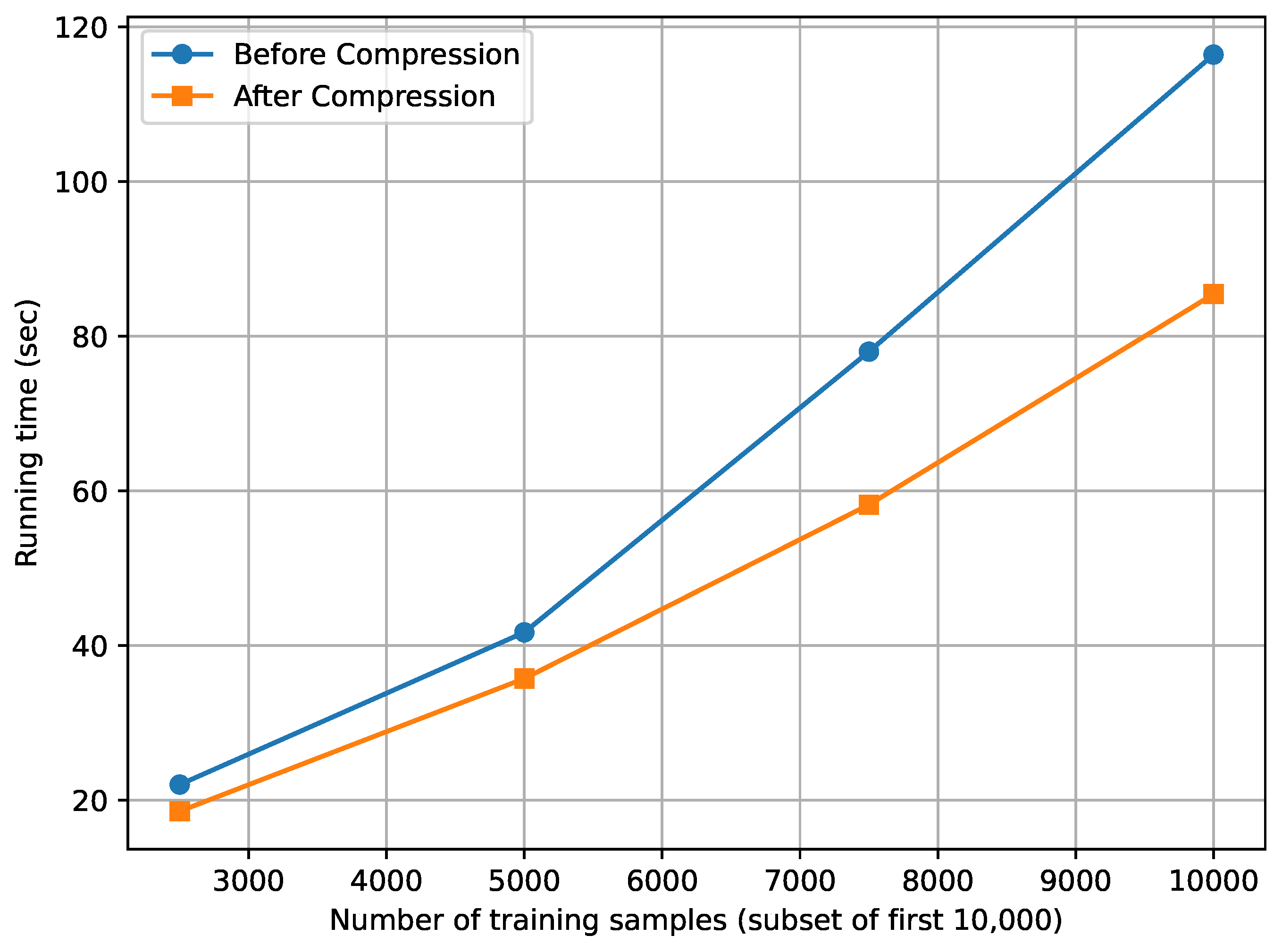
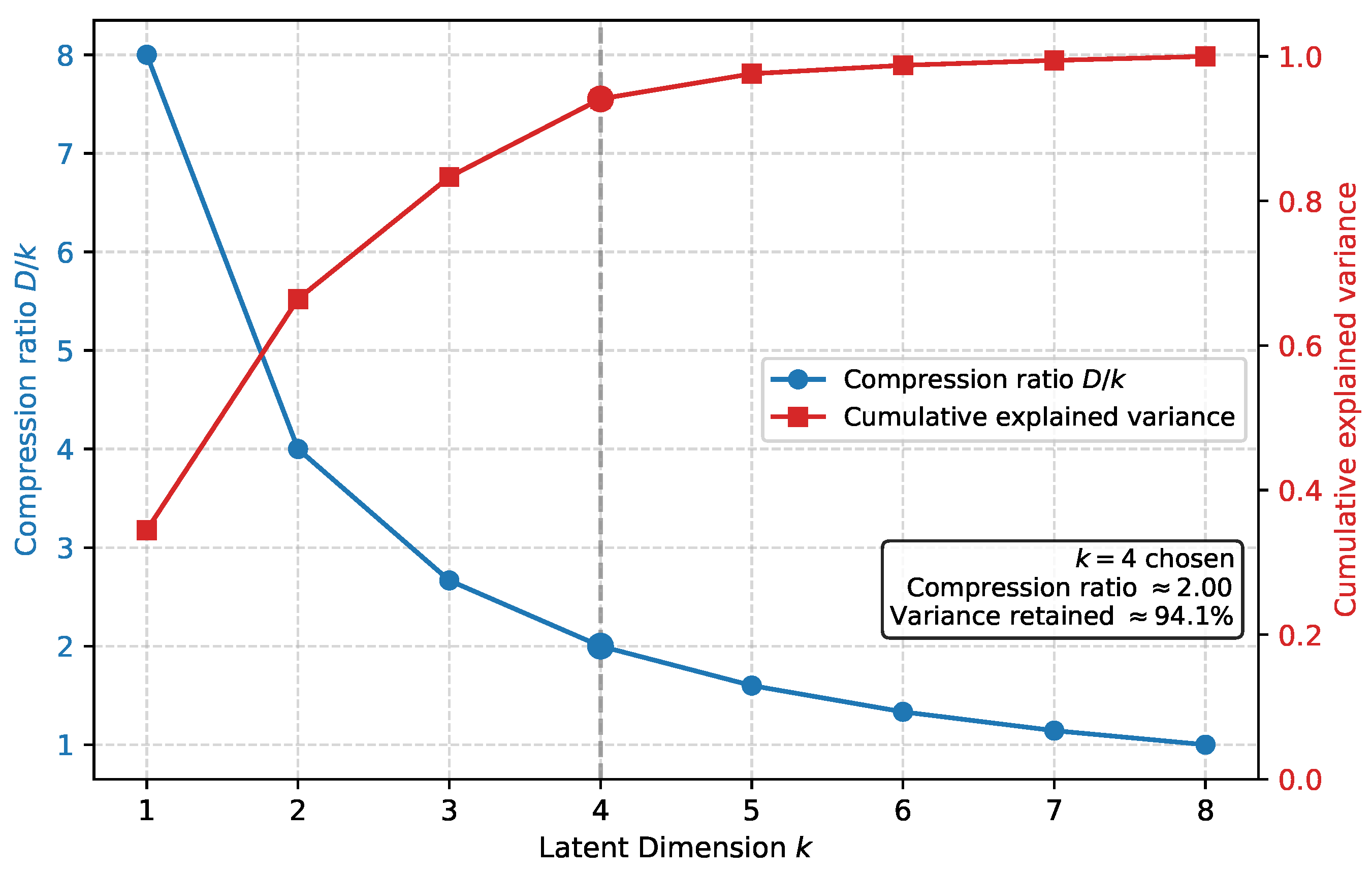
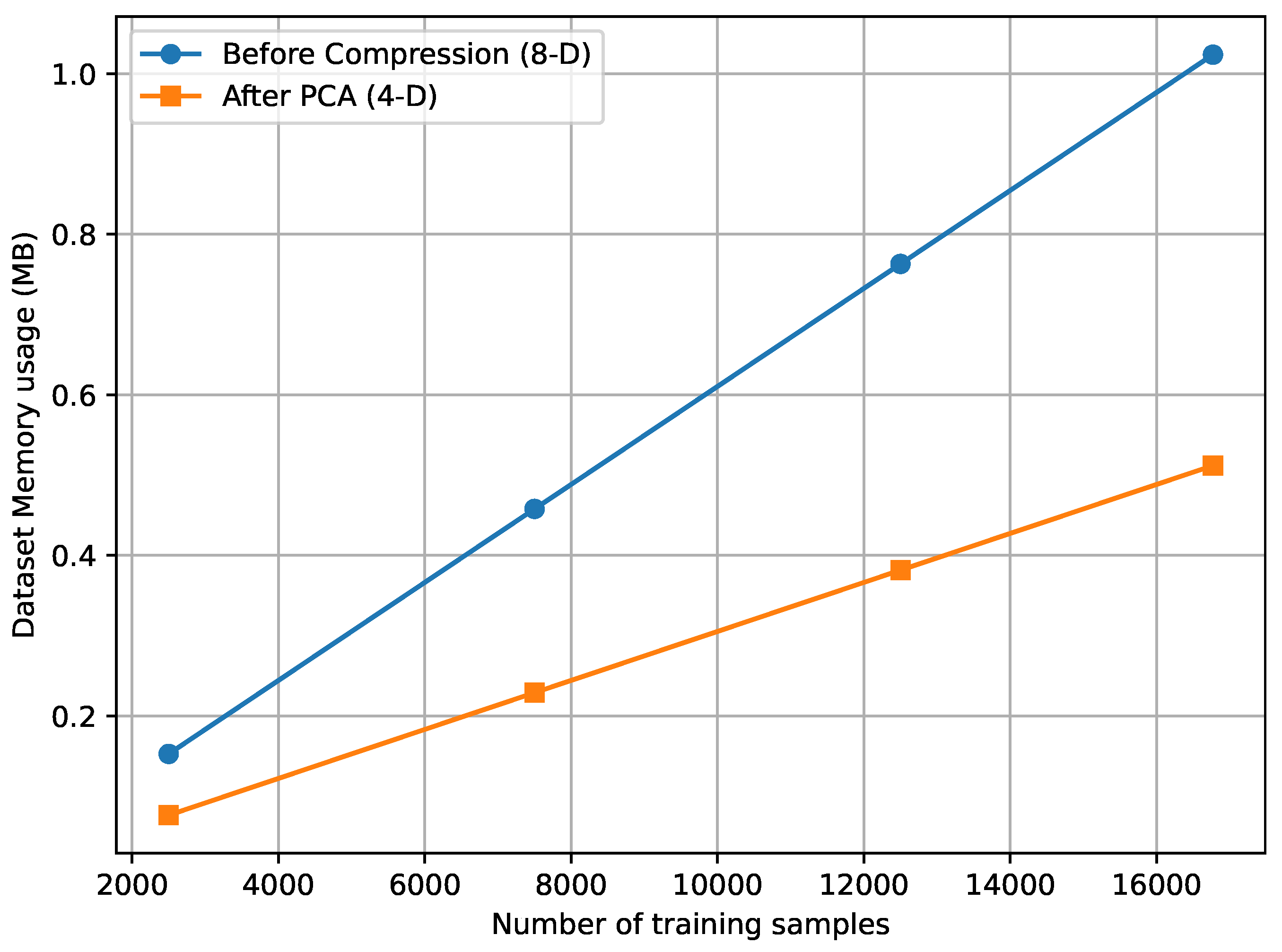
In this analysis, we evaluate the significance of feature compression within the SCENE-VLP pipeline, with a focus on information preservation and computational efficiency. Feature compression is implemented using dimensionality reduction methods, such as PCA and DAE. In the current setting, the latent dimension is fixed to four, yielding a compression ratio of 2 while retaining more than 90% of the original variance as shown in Figure 2. This indicates that most of the relevant information can be preserved while redundant feature components are removed. Figure 3 shows that the training runtime decreases after compression, with the reduction becoming more pronounced for larger training sets. Moreover, Figure 4 demonstrates that memory usage scales more efficiently when the dimensionality is reduced, since the feature representation occupies only half of the original space. Overall, the adoption of a four-dimensional latent space provides a balanced trade-off between information retention and computational complexity, reducing both runtime and memory requirements. These findings highlight the value of PCA (and similarly DAE) as a practical compression mechanism for SCENE-VLP, particularly for large-scale data, and motivate further investigation of its impact on downstream positioning performance in subsequent sections.

4.4. Training Data Requirements for Reliable Recurrent Learning

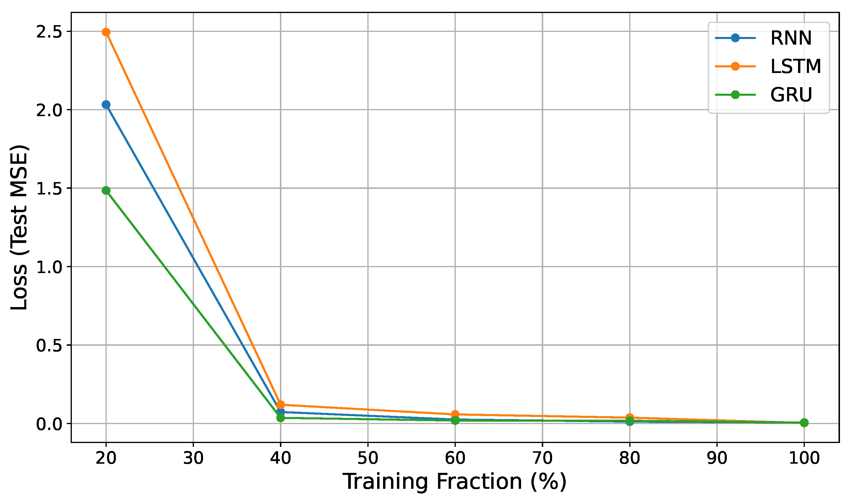
To evaluate how data availability influences the learning capability of recurrent architectures, we examined the behavior of RNN-based models across training fractions ranging from 20% to 100%. As shown in Figure 5, the test MSE decreases steadily for all models as more training data are provided, demonstrating smoother temporal feature learning with larger sample sizes. The most notable improvements occur once the training proportion exceeds 40%, where all recurrent models begin to converge more consistently and exhibit substantially reduced error. This observation highlights that the recurrent backbone used in SCENE-VLP benefits significantly from moderate to high data coverage, reinforcing the importance of sufficient training samples before introducing the complete system components presented in the subsequent sections.

4.5. RNN Architectures Leveraging PCA-Derived Orthogonal Feature Components

This subsection evaluates the performance of RNN architectures within the SCENE_ VLP framework when PCA-based dimensionality reduction is applied, as described in Section 3.2 and Section 3.3. The objective is to assess how different neural architectures exploit linearly compressed RSS features and to establish a clear performance reference prior to introducing probabilistic filtering.

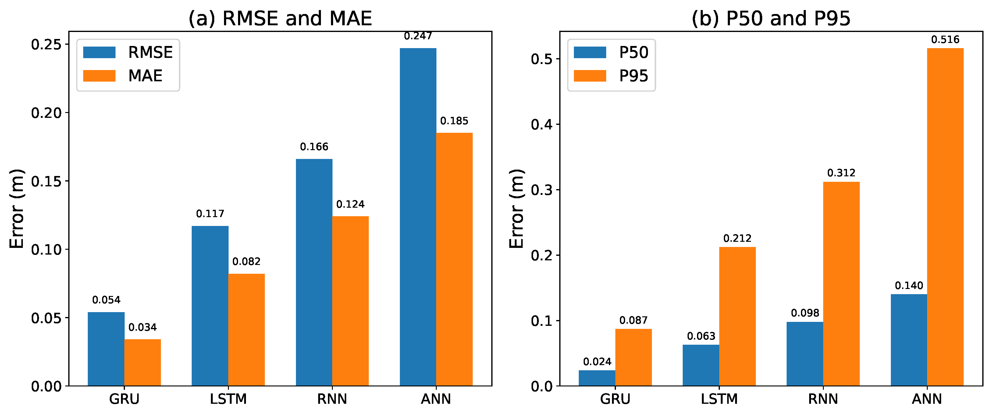
Figure 6 compares the proposed GRU-based sequential estimator with several widely used neural-network reference models, including a feedforward neural network, a simple RNN, and an LSTM. Feedforward neural networks are commonly employed in RSS-based indoor positioning as static nonlinear regressors [14], whereas recurrent architectures such as RNNs and LSTMs have demonstrated improved localization accuracy by explicitly modeling temporal dependencies in sequential RSS measurements [15,26]. To ensure a fair and transparent comparison, all reference models are trained and evaluated using identical PCA-compressed RSS features with a latent dimension of four, the same training and test datasets, and a fixed sequence length of ten time steps. The feedforward neural network operates on individual RSS snapshots without temporal memory, while the RNN, LSTM, and GRU exploit temporal correlations across consecutive measurements. The model configurations are kept consistent across recurrent architectures: each employs two recurrent layers with 180 and 90 hidden units, respectively, followed by identical dense output layers, as summarized in Table 1.

As shown in Figure 6, the GRU achieves the lowest training RMSE and MAE, at 5.4 cm and 3.4 cm, respectively. It also attains the smallest P50 and P95 errors of 2.4 cm and 8.7 cm, indicating improved robustness relative to the LSTM and RNN, while the feedforward neural network yields the highest errors. These results highlight the effectiveness of gated recurrent architectures in capturing temporal correlations when operating on PCA-compressed RSS features, which primarily preserve dominant linear signal components. However, PCA is inherently limited in representing nonlinear signal distortions commonly encountered in realistic indoor environments. To address this limitation, the next subsection investigates the use of DAE-based latent feature representations.

4.6. RNN Architectures Using DAE-Based Latent Feature Representations

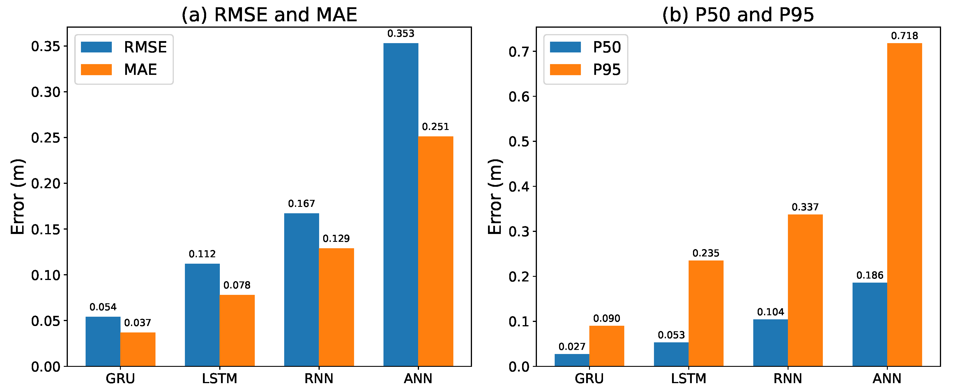
Building on the PCA-based analysis, this subsection evaluates the same set of baseline neural architectures (ANN, RNN, LSTM, and GRU) within the SCENE_VLP framework using DAE-derived latent feature representations, as outlined in Section 3.3 and Section 3.2. The training results in Figure 7 show that the GRU attains lower RMSE and MAE values of 5.4 cm and 3.7 cm, respectively, without the application of probabilistic filtering. The corresponding P50 and P95 values during training are 2.7 cm and 9 cm, while the LSTM and RNN architectures provide moderate performance, and the ANN produces higher errors. These outcomes demonstrate how recurrent models respond to DAE-derived latent features, which capture nonlinear signal characteristics. Therefore, the subsequent section incorporates probabilistic filtering methods to further enhance robustness and to assess their impact on temporal consistency and localization accuracy.

4.7. Impact of Filtering on PCA- and DAE-Based GRU Models

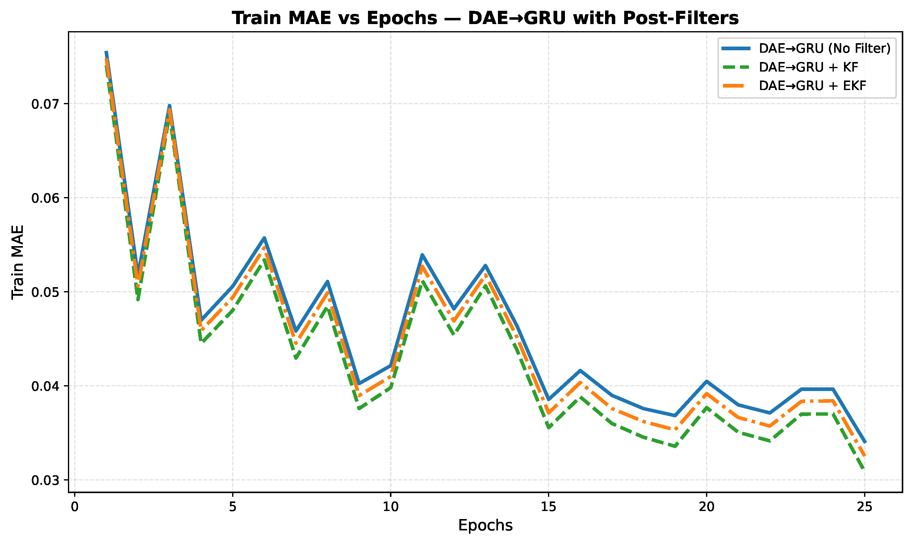
To evaluate the role of probabilistic filtering within SCENE-VLP, we compare KF and EKF refinements applied to PCA- and DAE-based GRU estimators. The purpose of this analysis is not to present EKF as a replacement for KF, but to examine how linear and nonlinear state-space refinements interact with a learned temporal measurement model. Quantitative results are reported in

Table 2. Training performance of PCA- and DAE-based GRU models under KF and EKF configurations (errors in cm, R² in %).

Model	P50 (cm)	P95 (cm)	RMSE (cm)	MAE (cm)	R2 (%)
PCA→GRU+KF	2.14	8.14	4.17	2.94	99.45
DAE→GRU+KF	2.09	6.98	3.68	2.69	99.55
PCA→GRU+EKF	2.02	7.97	4.10	2.91	99.83
DAE→GRU+EKF	1.84	6.52	3.58	2.64	99.87

, while distributional behavior and training dynamics are illustrated in Figure 8 and Figure 9. For the PCA→GRU pipeline, introducing KF reduces RMSE from 5.40 cm (no filtering) to 4.17 cm, with EKF providing a further refinement to 4.10 cm. A similar pattern is observed for MAE (2.94 cm with KF versus 2.91 cm with EKF) and for the tail error P95 (8.14 cm versus 7.97 cm). For the DAE→GRU chain, the impact of filtering is more pronounced: RMSE decreases from 5.43 cm (no filtering) to 3.68 cm with KF and 3.58 cm with EKF, while P95 decreases from 6.98 cm to 6.52 cm. These results demonstrate that recursive filtering substantially enhances robustness relative to the unfiltered GRU output, with EKF providing an additional incremental improvement when nonlinear effects are present.

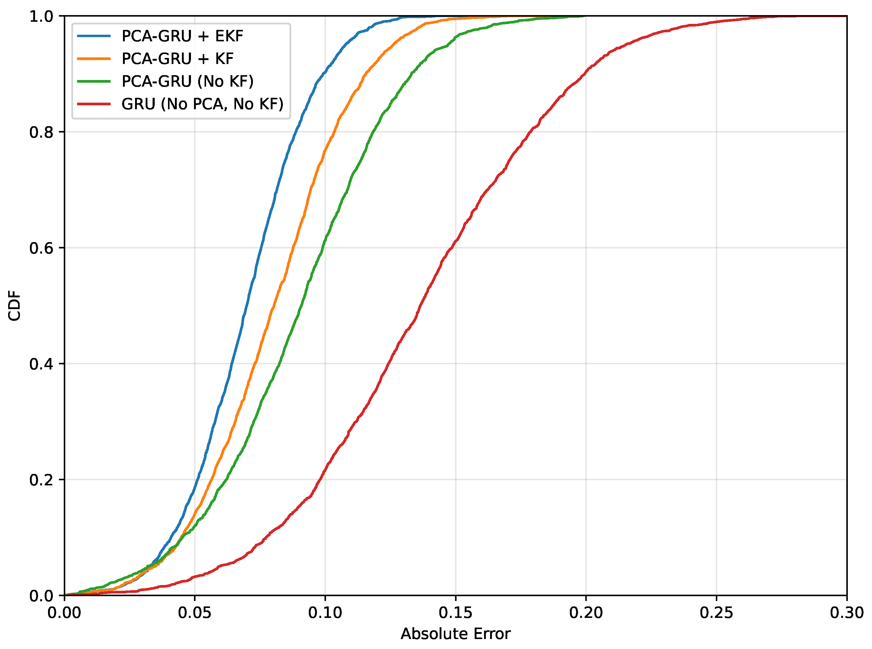
The CDF of absolute error (Figure 8) further confirms this behavior: both KF and EKF curves shift left relative to the unfiltered baseline, indicating that a larger proportion of samples falls within small error bounds. The difference between KF and EKF remains modest but consistent, particularly in the high-accuracy region (below 10 cm), where EKF exhibits slightly steeper convergence toward unity probability. Training dynamics provide complementary evidence. As shown in Figure 9, both KF and EKF reduce MAE trajectories compared to the unfiltered DAE→GRU configuration, with EKF producing marginally smoother and consistently lower curves across epochs. This behavior reflects the role of recursive state correction in stabilizing temporal predictions through motion constraints and uncertainty propagation.

Importantly, the improvement between KF and EKF is expected to be moderate in this setting: the adopted motion model is low-dimensional and largely well approximated by linear dynamics, so KF already captures most of the benefit of recursive state correction. EKF acts as a principled extension that can accommodate mild nonlinearities in the effective observation/measurement relationship arising from indoor optical channel effects and the learned measurement mapping, yielding incremental but systematic gains rather than dramatic differences. To assess whether these improvements are statistically meaningful, we conducted multi-run evaluations across multiple random seeds and computed 95% confidence intervals for RMSE. In all configurations, the mean RMSE obtained with EKF was lower than that of KF, and for the DAE-based models the confidence intervals showed consistent separation, indicating that the observed improvements are repeatable rather than incidental.

4.8. Component Contribution Analysis

To rigorously validate the contribution of each module in the proposed PCA/DAE–GRU–EKF framework, we conduct a structured ablation study across three evaluation settings: Scenario A (Dataset1), Scenario B (Dataset2), and Scenario C (train on Dataset1, test on Dataset2). The detailed numerical results are reported in Table 3, Table 4 and Table 5. All errors are expressed in centimeters (cm), and lower values indicate better performance.

4.8.1. Compression: PCA vs. DAE

The quantitative comparison between PCA and DAE under a GRU backbone without filtering is summarized in Table 3. The impact of feature compression varies across scenarios. In Scenario A, PCA+GRU achieves lower RMSE (9.30 cm) and P95 (23.10 cm) than DAE+GRU (17.46 cm and 39.17 cm), indicating that linear variance-preserving projection is sufficient under structured industrial measurements. In Scenario B, the trend reverses: DAE+GRU reduces RMSE from 12.59 cm (PCA) to 6.18 cm and lowers P95 from 20.42 cm to 12.96 cm, demonstrating improved robustness under heterogeneous measurement conditions. In cross-dataset Scenario C, DAE again yields lower RMSE (4.36 cm vs. 4.51 cm) and P95 (8.25 cm vs. 8.79 cm), indicating improved tail-error robustness and competitive median accuracy under environment shift.

Table 3. Effect of feature compression (PCA vs. DAE) across scenarios (GRU backbone, no filtering). Errors in cm.

Scenario	Compression	MAE (cm)	RMSE (cm)	P50 (cm)	P95 (cm)
Scenario A	PCA	6.44	9.30	3.74	23.10
	DAE	11.49	17.46	6.09	39.17
Scenario B	PCA	7.32	12.59	4.90	20.42
	DAE	4.73	6.18	3.62	12.96
Scenario C	PCA	3.01	4.51	2.28	8.79
	DAE	3.06	4.36	2.21	8.25

Table 3. Effect of feature compression (PCA vs. DAE) across scenarios (GRU backbone, no filtering). Errors in cm.

Scenario	Compression	MAE (cm)	RMSE (cm)	P50 (cm)	P95 (cm)
Scenario A	PCA	6.44	9.30	3.74	23.10
	DAE	11.49	17.46	6.09	39.17
Scenario B	PCA	7.32	12.59	4.90	20.42
	DAE	4.73	6.18	3.62	12.96
Scenario C	PCA	3.01	4.51	2.28	8.79
	DAE	3.06	4.36	2.21	8.25

4.8.2. Temporal Modeling: GRU vs. Feedforward

The quantitative comparison between GRU and feedforward modeling is summarized in Table 4. Across all scenarios, the GRU consistently outperforms the FFNN baseline. In Scenario A, RMSE decreases from 10.11 cm (Raw+FFNN) to 9.80 cm (Raw+GRU), and P95 reduces from 24.65 cm to 23.32 cm. In Scenario B, RMSE decreases from 13.36 cm to 12.59 cm, while P50 improves from 5.52 cm to 4.90 cm. The most noticeable improvement is observed in Scenario C, where RMSE decreases from 5.18 cm to 4.88 cm and P95 from 11.43 cm to 9.91 cm. These consistent reductions in both average (MAE, RMSE) and P95 errors confirm that temporal dependency learning provides measurable gains over static regression, particularly under cross-environment conditions.

Table 4. Effect of temporal modeling (GRU vs. FFNN) across scenarios (no filtering). Errors in cm.

Scenario	Model	MAE (cm)	RMSE (cm)	P50 (cm)	P95 (cm)
Scenario A	Raw+FFNN	7.67	10.11	5.94	24.65
	Raw+GRU	6.68	9.80	4.57	23.32
Scenario B	Raw+FFNN	7.8	13.36	5.52	22.49
	Raw+GRU	7.32	12.59	4.90	21.01
Scenario C	Raw+FFNN	4.02	5.18	4.32	11.43
	Raw+GRU	3.12	4.88	3.71	9.91

Table 4. Effect of temporal modeling (GRU vs. FFNN) across scenarios (no filtering). Errors in cm.

Scenario	Model	MAE (cm)	RMSE (cm)	P50 (cm)	P95 (cm)
Scenario A	Raw+FFNN	7.67	10.11	5.94	24.65
	Raw+GRU	6.68	9.80	4.57	23.32
Scenario B	Raw+FFNN	7.8	13.36	5.52	22.49
	Raw+GRU	7.32	12.59	4.90	21.01
Scenario C	Raw+FFNN	4.02	5.18	4.32	11.43
	Raw+GRU	3.12	4.88	3.71	9.91

4.8.3. Sequential-Only vs. Compression-Only vs. Full Integration

A comparison of partial and complete pipelines further clarifies the benefit of structured integration. As shown in Table 5, sequential-only modeling (GRU on raw RSS) already provides competitive accuracy across all scenarios, confirming the importance of temporal dependency learning. In Scenario A, the raw GRU achieves RMSE of 9.80 cm and P95 of 23.32 cm. Applying PCA reduces these values to 9.30 cm and 20.10 cm, respectively. With EKF refinement, RMSE further decreases to 7.87 cm and P95 to 17.15 cm. In Scenario B, PCA+GRU provides only marginal improvement over the raw GRU, whereas PCA+GRU+EKF significantly lowers RMSE to 5.14 cm and P95 to 11.29 cm. In Scenario C, the raw GRU yields RMSE of 4.88 cm and P95 of 5.91 cm. The full PCA+GRU+EKF configuration achieves the lowest RMSE of 4.10 cm, improves median accuracy (P50 = 2.02 cm), and maintains controlled tail error (P95 = 7.97 cm). Across all scenarios, the integrated PCA+GRU+EKF configuration consistently achieves the lowest RMSE and MAE values compared to partial pipelines.

Table 5. Sequential-only vs. compression-only vs. full integration across scenarios. Errors in cm.

Scenario	Model	MAE (cm)	RMSE (cm)	P50 (cm)	P95 (cm)
Scenario A	GRU (Raw RSS)	6.68	9.80	4.57	23.32
	PCA+GRU	6.44	9.30	3.74	20.10
	PCA+GRU+EKF	5.50	7.87	3.58	17.15
Scenario B	GRU (Raw RSS)	7.32	12.59	4.90	21.01
	PCA+GRU	6.90	12.47	4.36	20.42
	PCA+GRU+EKF	3.69	5.14	2.76	11.29
Scenario C	GRU (Raw RSS)	3.12	4.88	3.71	9.91
	PCA+GRU	3.01	4.51	2.28	8.79
	PCA+GRU+EKF	2.91	4.10	2.02	7.97

Table 5. Sequential-only vs. compression-only vs. full integration across scenarios. Errors in cm.

Scenario	Model	MAE (cm)	RMSE (cm)	P50 (cm)	P95 (cm)
Scenario A	GRU (Raw RSS)	6.68	9.80	4.57	23.32
	PCA+GRU	6.44	9.30	3.74	20.10
	PCA+GRU+EKF	5.50	7.87	3.58	17.15
Scenario B	GRU (Raw RSS)	7.32	12.59	4.90	21.01
	PCA+GRU	6.90	12.47	4.36	20.42
	PCA+GRU+EKF	3.69	5.14	2.76	11.29
Scenario C	GRU (Raw RSS)	3.12	4.88	3.71	9.91
	PCA+GRU	3.01	4.51	2.28	8.79
	PCA+GRU+EKF	2.91	4.10	2.02	7.97

4.9. Computational Complexity and Feasibility

As described in the system model presented in Section 3, the proposed framework separates offline learning from online inference. Feature compression learning, recurrent neural network training, and filter parameter tuning are carried out offline using the available dataset. During online operation, the system performs only forward inference through the trained models and recursive state estimation. Let L denote the number of LEDs, k the latent feature dimension, T the sequence length, h the number of recurrent hidden units, and s the EKF state dimension. Based on the processing steps defined in Section 3, the computational complexity of the online processing per time step can be expressed as

$$\mathcal{O}\left(Lk+T(h^2+hk)+s^3\right),$$

(29)

where the first term corresponds to feature encoding, the second term accounts for recurrent neural network inference over a sequence of length T, and the third term represents the computational cost of the EKF update. In the proposed configuration, all quantities are fixed and low dimensional. The online computational complexity is independent of the size of the training dataset, since no fingerprint search, kernel evaluation, or iterative optimization is performed during inference. The EKF operates on a low-dimensional state vector, and its computational overhead is small relative to the recurrent inference stage.

4.10. Cross-Environment Analysis

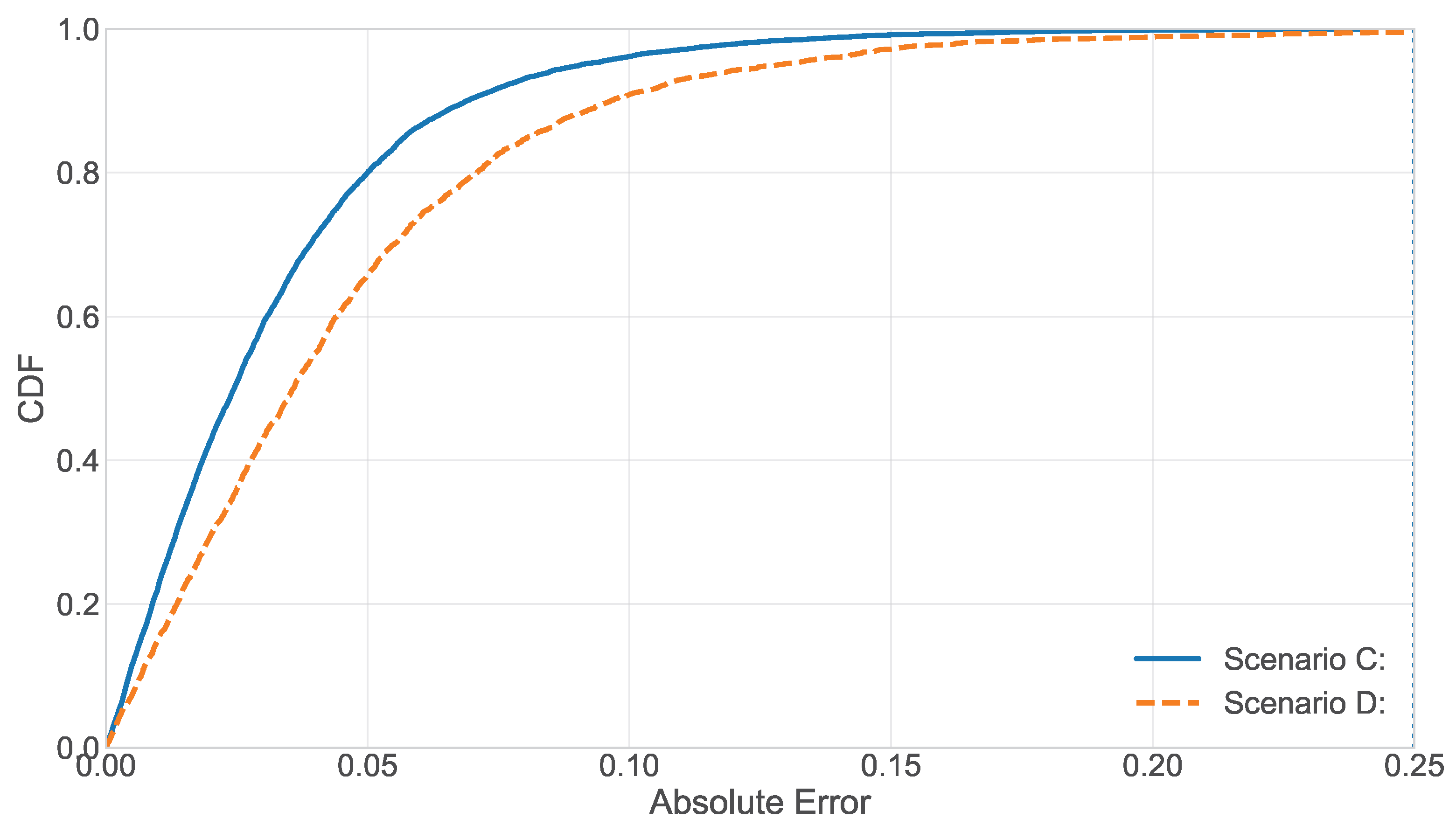
To evaluate the scalability and robustness of the proposed model, simulations are also conducted on a public VLP dataset reported in [27]. The key experimental characteristics of both datasets are summarized in

Table 6. Experimental dataset characteristics for cross-environment model evaluation.

Parameter	SCENE-VLP Dataset	Public-VLP Dataset
Environment type	Industrial indoor logistics environment	Office-like open indoor environment
Room dimensions	$12\mathrm{m}\times 18\mathrm{m}\times 6.81\mathrm{m}$	$6.3\mathrm{m}\times 6.9\mathrm{m}\times 2.4\mathrm{m}$
Receiver height	$1.1\mathrm{m}$	≈1.0 $\mathrm{m}$
Number of LED/PD	8/1	11/1
LED deployment	Rectangular constellation	Distributed ceiling luminaires
Signal features	RSS (FDMA-separated intensities)	RSS (frequency-coded intensities)
Ground-truth system	Industrial LIDAR localization	HTC Vive VR tracking
Number of measurement points	D1: 19,359/D2: 16,770	7344
Sampling strategy	Realistic movement trajectories	Autonomous robotic fingerprinting
Obstacles/NLOS conditions	Yes (machines, walls)	Yes (structural pillar)

, highlighting differences in spatial scale, ceiling height, LED deployment, sampling strategy, and ground-truth systems. Scenario C corresponds to the dataset used in the SCENE-VLP framework, collected in an industrial logistics hall [25], while Scenario D corresponds to the publicly available Public-VLP dataset acquired in an office-like indoor environment [27]. The substantial differences between these datasets result in distinct RSS distributions and propagation conditions. Although stable convergence is observed for both scenarios during training and validation, loss metrics alone do not fully characterize localization performance across heterogeneous environments. Therefore, the CDF of absolute positioning errors is used to provide a more informative performance comparison. Figure 10 illustrates the CDF results obtained for Scenario C and Scenario D under the same model configuration. The CDF results indicate that approximately 50% of the samples in Scenario C are localized within about 5 cm, whereas the same confidence level in Scenario D is reached at around 7 cm. Similarly, about 95% of the samples in Scenario C fall below an error of approximately 14 cm, compared to about 18 cm in Scenario D, indicating higher localization reliability in Scenario C. The left-shifted CDF curve of Scenario C further indicates that a larger proportion of test samples achieves smaller localization errors. The observed performance difference can be attributed to the structured measurement trajectories and consistent receiver height in the industrial dataset, whereas the Public-VLP dataset introduces additional variability due to autonomous motion, heterogeneous signal incidence angles, and more diverse sampling paths. Nevertheless, both scenarios exhibit steep initial CDF slopes, with the majority of test samples localized within a low-error range, indicating reliable performance in both environments.

4.11. Benchmarking SCENE-VLP Against Existing Approaches

To contextualize SCENE-VLP within the broader landscape of indoor VLP research, this subsection compares its performance with representative learning-based approaches summarized in

Table 7. Comparative positioning performance among related works (values are taken from the respective published papers).

Comparison	Fite et al. (SCENE-VLP)	Yang et al. [15]	Wu et al. [28]	De Bruycker et al. [29]	Garbuglia et al. [30]
Core method	SCENE (trajectory smoothing and occlusion-tolerant)	GRU	DKL + BN	GP/SVM/NN/XGBoost	Bayesian Active Learning + GP
Environment size (m)	$6\times 12\times 5.71$	$4\times 4\times 3$ (sim.)	$6\times 12\times 5.71$	$8\times 8$ (sim.)	$6\times 4$ (exp.)
Tx/Rx setup	8 LEDs and 1 PD	2 LEDs and 3 PDs	8 LEDs and 1 PD	4 LEDs and 1 PD	4 LEDs and 1 PD
Dynamic consideration	Yes (motion + occlusion)	LOS + NLOS	Real movement trajectories	Shadowing analyzed	Data-efficient offline model construction
Feature compression	PCA/DAE	None	MLP extractor	None	None
Sequential modeling	RNN (GRU)	GRU	None	None	None
Filtering/tracking	KF/EKF	None	None	None	None
P50 (cm)	1.84	–	2.56	–	–
P95 (cm)	6.52	7.88	6.87	9.87 (GP, obstacles)	≈10.0 (GP)
Mean (cm)	2.01	2.66	3.34	3.00 (GP)	≈3.2 (GP)

. The reported values are taken directly from the respective published works and are compared while accounting for differences in environment scale, sensing configuration, and algorithmic design. The selected comparison methods were chosen to represent complementary and widely adopted research directions in VLP, rather than to exhaustively enumerate all existing approaches. Specifically, Yang et al. [15] represent sequence-learning-based RSS regression using GRU networks; Wu et al. [28] reflect kernel-based deep regression models evaluated in a large-scale experimental environment; De Bruycker et al. [29] provide an obstacle-aware benchmarking study of static machine learning regressors; and Garbuglia et al. [30] focus on data-efficient offline model construction via Bayesian active learning. Together, these methods cover key methodological categories in the VLP literature, including sequential learning, kernel-based regression, obstacle analysis, and data efficiency.

SCENE-VLP achieves a P50 of 1.84 cm, a P95 of 6.52 cm, and a mean error of 2.01 cm in a large and dynamic $6\times 12\times 5.71$ m environment with a single photodetector. This performance reflects the combined effect of PCA/DAE-based feature compression, GRU-based temporal modeling, and EKF-based state refinement, which together enable trajectory smoothing and robustness against motion- and occlusion-induced disturbances. In contrast, Yang et al. [15] employ a GRU-based sequential RSS regression model to improve positioning accuracy under LOS and NLOS conditions in a smaller simulated $4\times 4\times 3$ m environment. While their approach benefits from temporal learning, the absence of probabilistic tracking or state refinement results in a higher mean error of 2.66 cm and a wider error tail, with a reported P95 of 7.88 cm. Wu et al. [28] report P50, P95, and mean errors of 2.56 cm, 6.87 cm, and 3.34 cm, respectively, using a Deep Kernel Learning model with Batch Normalization (DKL+BN) in an environment of the same scale as SCENE-VLP. Although DKL+BN enhances regression generalization, the lack of explicit sequential modeling and filtering limits its ability to suppress temporal error accumulation. De Bruycker et al. [29] focus on obstacle-aware RSS-based VLP by benchmarking multiple static machine learning regressors in an $8\times 8$ m simulated environment. Their reported P95 of approximately 9.87 cm under obstacle conditions highlights the limitations of frame-based regression without temporal modeling or tracking. Similarly, Garbuglia et al. [30] investigate Bayesian active learning to reduce training data requirements for GP-based RSS positioning. While effective for offline data-efficient model construction, the resulting localization model operates as a static regressor and does not address trajectory smoothing or online tracking.

5. Conclusions

This study introduced SCENE-VLP, a unified framework for indoor visible light positioning that combines feature compression, temporal modeling, and probabilistic state-space refinement. The method was evaluated across three scenarios, including same-dataset and cross-dataset settings, ensuring validation under both nominal and domain-shift conditions. Results show that PCA and DAE effectively condition the RSS observation space while reducing dimensionality, with a latent dimension of four providing an efficient trade-off between information retention and computational cost. The ablation analysis confirms that GRU-based temporal modeling improves robustness over static regression, particularly under motion and signal variability. Recursive filtering further enhances accuracy, with Kalman-based refinement consistently reducing positioning errors compared to unfiltered GRU outputs. The comparison between KF and EKF indicates that the primary improvement stems from recursive state correction itself, while EKF delivers systematic but moderate gains when nonlinearities are present. Across all scenarios, SCENE-VLP achieves sub-decimeter performance in a realistic industrial environment, with P50 of 1.84 cm and P95 of 6.52 cm. Cross-dataset evaluation further demonstrates stable generalization. Overall, the conclusions are directly supported by multi-scenario experiments, structured ablation analysis, and statistical validation. The results confirm that observation conditioning, temporal dependency learning, and Bayesian state refinement act as complementary components within a principled hierarchical estimation framework. Future work will extend SCENE-VLP to 3D positioning, multi-sensor fusion, physics-informed neural networks, and transfer learning across heterogeneous indoor environments.

References

1. Aziz, T.; Koo, I. A Comprehensive Review of Indoor Localization Techniques and Applications in Various Sectors. Appl. Sci. 2025, 15, 1544. [Google Scholar] [CrossRef] [Scilit]
2. Bakar, A.H.A.; Glass, T.; Tee, H.Y.; Alam, F.; Legg, M. Accurate Visible Light Positioning Using Multiple-Photodiode Receiver and Machine Learning. IEEE Trans. Instrum. Meas. 2020, 70, 7500812. [Google Scholar] [CrossRef] [Scilit]
3. Shi, L.; Shi, D.; Zhang, X.; Meunier, B.; Zhang, H.; Wang, Z.; Vladimirescu, A.; Li, W.; Zhang, Y.; Cosmas, J.; et al. 5G Internet of Radio Light Positioning System for Indoor Broadcasting Service. IEEE Trans. Broadcast. 2020, 66, 534–544. [Google Scholar] [CrossRef] [Scilit]
4. Ghassemlooy, Z.; Popoola, W.; Rajbhandari, S. Optical Wireless Communications; CRC Press: Boca Raton, FL, USA, 2019. [Google Scholar] [CrossRef] [Scilit]
5. Gu, W.; Aminikashani, M.; Deng, P.; Kavehrad, M. Impact of Multipath Reflections on the Performance of Indoor Visible Light Positioning Systems. J. Light. Technol. 2016, 34, 2578–2587. [Google Scholar] [CrossRef] [Scilit]
6. Lain, J.K.; Chen, L.C.; Lin, S.C. Indoor Localization Using K-Pairwise Light Emitting Diode Image-Sensor-Based Visible Light Positioning. IEEE Photonics J. 2018, 10, 1–9. [Google Scholar] [CrossRef] [Scilit]
7. Rekkas, V.P.; Sotiroudis, S.P.; Iliadis, L.A.; Bastiaens, S.; Joseph, W.; Plets, D.; Christodoulou, C.G.; Karagiannidis, G.K.; Goudos, S.K. Enhancing 3D Indoor Visible Light Positioning with Machine Learning Combined Nyström Kernel Approximation. IEEE Trans. Broadcast. 2024, 70, 1192–1206. [Google Scholar] [CrossRef] [Scilit]
8. Chaudhary, N.; Alves, L.N.; Ghassemlooy, Z. Impact of Transmitter Positioning and Orientation Uncertainty on RSS-Based Visible Light Positioning Accuracy. Sensors 2021, 21, 3044. [Google Scholar] [CrossRef] [Scilit]
9. Xu, S.; Wu, Y.; Wang, X.; Wei, F. Indoor High Precision Positioning System Based on Visible Light Communication and Location Fingerprinting. J. Light. Technol. 2023, 41, 5564–5576. [Google Scholar] [CrossRef] [Scilit]
10. Wang, R.; Niu, G.; Cao, Q.; Chen, C.S.; Ho, S.W. A Survey of Visible-Light-Communication-Based Indoor Positioning Systems. Sensors 2024, 24, 5197. [Google Scholar] [CrossRef] [Scilit] [PubMed]
11. Palitharathna, K.W.S.; Wickramasinghe, N.D.; Vegni, A.M.; Suraweera, H.A. Neural Network-Based Optimization for SLIPT-Enabled Indoor VLC Systems with Energy Constraints. IEEE Trans. Green Commun. Netw. 2024, 8, 839–851. [Google Scholar] [CrossRef] [Scilit]
12. Chaudhary, N.; Othman, I.Y.; Zvanovec, S. The Usage of ANN for Regression Analysis in Visible Light Positioning Systems. Sensors 2022, 22, 2879. [Google Scholar] [CrossRef] [Scilit] [PubMed]
13. Plets, D.; Almadani, Y.; Bastiaens, S.; Ijaz, M. Efficient 3D Trilateration Algorithm for Visible Light Positioning. J. Opt. 2019, 21, 05LT01. [Google Scholar] [CrossRef] [Scilit]
14. Raes, W.; Knudde, N.; De Bruycker, J.; Dhaene, T.; Stevens, N. Experimental Evaluation of Machine Learning Methods for Robust Received Signal Strength-Based Visible Light Positioning. Sensors 2020, 20, 6109. [Google Scholar] [CrossRef] [Scilit] [PubMed]
15. Yang, W.; Qin, L.; Hu, X.; Zhao, D. Indoor Visible-Light 3D Positioning System Based on GRU Neural Network. Photonics 2023, 10, 633. [Google Scholar] [CrossRef] [Scilit]
16. Gufran, D.; Tiku, S.; Pasricha, S. SANGRIA: Stacked Autoencoder Neural Networks with Gradient Boosting for Indoor Localization. IEEE Embed. Syst. Lett. 2024, 16, 142–145. [Google Scholar] [CrossRef] [Scilit]
17. Tian, Y.; Lian, Z.; Wang, P.; Wang, M.; Yue, Z.; Chai, H. Application of a long short-term memory neural network algorithm fused with Kalman filter in UWB indoor positioning. Sci. Rep. 2024, 14, 1925. [Google Scholar] [CrossRef] [Scilit]
18. Mao, X.; Jing, L.; Tong, Z.; Zhang, W.; Li, P.; Wang, X.; Wang, H.; Cao, T.; Sun, Z. Indoor visible light positioning system driven by deep neural network based on Kalman filtering and clustering optimization. Opt. Commun. 2025, 591, 132090. [Google Scholar] [CrossRef] [Scilit]
19. Jolliffe, I.T.; Cadima, J. Principal Component Analysis: A Review and Recent Developments. Philos. Trans. R. Soc. A 2016, 374, 20150202. [Google Scholar] [CrossRef] [Scilit]
20. Kim, K.; Lee, J. Adaptive Scheme of Denoising Autoencoder for Estimating Indoor Localization Based on RSSI Analytics in BLE Environment. Sensors 2023, 23, 5544. [Google Scholar] [CrossRef] [Scilit]
21. Cho, K.; Van Merriënboer, B.; Gulcehre, C.; Bahdanau, D.; Bougares, F.; Schwenk, H.; Bengio, Y. Learning Phrase Representations Using RNN Encoder–Decoder for Statistical Machine Translation. In Proceedings of the 2014 Conference on Empirical Methods in Natural Language Processing (EMNLP), Doha, Qatar, 25–29 October 2014; pp. 1724–1734. [Google Scholar] [CrossRef] [Scilit]
22. Kalman, R.E. A New Approach to Linear Filtering and Prediction Problems. J. Basic Eng. 1960, 82, 35–45. [Google Scholar] [CrossRef] [Scilit]
23. Fite, N.B.; Wegari, G.M.; Steendam, H. Integration of Artificial Neural Network Regression and Principal Component Analysis for Indoor Visible Light Positioning. Sensors 2025, 25, 1049. [Google Scholar] [CrossRef] [Scilit] [PubMed]
24. Turan, B.; Kar, E.; Coleri, S. Vehicular Visible Light Communications Noise Analysis and Autoencoder Based Denoising. In Proceedings of the 2022 Joint European Conference on Networks and Communications and 6G Summit (EuCNC/6G Summit); IEEE: New York, NY, USA, 2022; pp. 19–24. [Google Scholar] [CrossRef] [Scilit]
25. Raes, W.; De Bruycker, J.; Stevens, N. A Cellular Approach for Large Scale, Machine Learning Based Visible Light Positioning Solutions. In Proceedings of the 2021 International Conference on Indoor Positioning and Indoor Navigation (IPIN); IEEE: New York, NY, USA, 2021; pp. 1–6. [Google Scholar] [CrossRef] [Scilit]
26. Shu, Y.H.; Chang, Y.H.; Lin, Y.Z.; Chow, C.W. Real-Time Indoor Visible Light Positioning (VLP) Using Long Short Term Memory Neural Network (LSTM-NN) with Principal Component Analysis (PCA). Sensors 2024, 24, 5424. [Google Scholar] [CrossRef] [Scilit] [PubMed]
27. Glass, T.; Alam, F.; Legg, M.; Noble, F. Autonomous Fingerprinting and Large Experimental Data Set for Visible Light Positioning. Sensors 2021, 21, 3256. [Google Scholar] [CrossRef] [Scilit]
28. Wu, F.; Stevens, N.; De Strycker, L.; Rottenberg, F. Comparative Study of Gaussian Processes, Multi Layer Perceptrons, and Deep Kernel Learning for Indoor Visible Light Positioning Systems. In Proceedings of the 2023 13th International Conference on Indoor Positioning and Indoor Navigation (IPIN 2023); IEEE: New York, NY, USA, 2023; pp. 1–6. [Google Scholar] [CrossRef] [Scilit]
29. De Bruycker, J.; Garbuglia, F.; Dhaene, T. Evaluation of Machine Learning Models for Received Signal Strength Based Visible Light Positioning with Obstacles. In Proceedings of the 14th International Symposium on Communication Systems, Networks and Digital Signal Processing (CSNDSP); IEEE: New York, NY, USA, 2024; pp. 318–323. [Google Scholar] [CrossRef] [Scilit]
30. Garbuglia, F.; Raes, W.; De Bruycker, J.; Stevens, N.; Deschrijver, D.; Dhaene, T. Bayesian Active Learning for Received Signal Strength-Based Visible Light Positioning. IEEE Photonics J. 2022, 14, 8559208. [Google Scholar] [CrossRef] [Scilit]
Figure 1. Overall architecture of the proposed SCENE_VLP framework. The system integrates feature compression, sequential modeling, and refinement.
Photonics 13 00211 g001
Figure 2. Compression trade-off between latent dimension, compression ratio, and cumulative explained variance.
Photonics 13 00211 g002
Figure 3. Training runtime versus number of samples before and after compression.
Photonics 13 00211 g003
Figure 4. Memory usage versus number of samples before and after compression.
Photonics 13 00211 g004
Figure 5. Impact of training sample size on the learning performance of recurrent architectures, showing that the proposed SCENE-VLP model achieves stable and low test MSE with as little as 40% training data.
Photonics 13 00211 g005
Figure 6. Training performance of recurrent models with PCA-based dimensionality reduction in the SCENE_VLP framework. Lower values indicate better accuracy (in meters).
Photonics 13 00211 g006
Figure 7. Training performance of recurrent models with DAE-based latent feature extraction in the SCENE_VLP framework. Lower values represent better accuracy (in meters).
Photonics 13 00211 g007
Figure 8. CDF of absolute positioning error for PCA→GRU with and without Kalman-based filtering and for the GRU baseline without PCA.
Photonics 13 00211 g008
Figure 9. Training MAE versus epochs for DAE→GRU under No Filter, KF, and EKF configurations.
Photonics 13 00211 g009
Figure 10. CDF of absolute positioning errors for cross-environment evaluation. Scenario C corresponds to the SCENE-VLP dataset, while Scenario D corresponds to the Public-VLP dataset, evaluated using the same model configuration.
Photonics 13 00211 g010