Abstract
The rotational Doppler effect (RDE) has been playing a vital role in the detection of rotational motion in recent years. However, the results obtained from this detection method are easily influenced by the detection conditions. It means that the characteristic of the frequency signals varies greatly under different detection conditions. How to efficiently and automatically classify and recognize different signal features is of great significance for the accurate extraction of rotating speed information in the future. Based on the well-known support vector machine (SVM) model, we built an SVM learn model to automatically classify and recognize RDE signals under different detection conditions. The results show that the SVM learn model can effectively recognize the category of detection signals with high accuracy. By accurately identifying signal categories, it can provide a great foundation for extracting target speed and other information in the future, and has broad application prospects in engineering practice.
1. Introduction
Since the first application of the RDE of the optical vortex (OV) beams to the measurement of the rotational speed of a real object by Padgett et al. in 2013 [1], researchers have conducted many studies on using vortex beams for target speed measurement in recent years. In 2014, Lavery et al. published their milestone experimental research results on achieving target speed measurement with orbital angular momentum (OAM) carrying white light in the inaugural article of Optica [2]. Afterwards, the concept of RDE further attracted people’s awareness [3,4,5,6,7]. In addition to the target rotational speed, the detection scheme based on superimposed vortex beams can also realize the measurement of rotational and linear motion speed simultaneously [8,9,10], which suggests that this effect may have important application potential in target measurement [11,12]. In 2019, we first proposed the concept of non-coaxial RDE [13], and further elucidated the mechanism of target speed detection under the condition that the axis of the vortex beam does not align with the rotating axis [14]. This study breaks the limitations of traditional measurement methods on beam irradiation pose and has operability in practical applications.
Although there have been many studies conducted according to RDE, so far, all of those observations still need to be based on frequency spectral analysis [15,16,17], as the Doppler effect is mainly reflected in the modulation of the frequency of the detection beam by object motion [17,18,19,20]. By collecting scattered light from the rotating target, obtaining the time-domain signal, and further performing spectral conversion through Fourier transformation (FFT), the motion information can be observed from the spectrum [19,21,22,23]. This method can solve the problem of extracting target rotation speed in most detection scenarios, but its disadvantage is that the processing is relatively complex, and it is difficult to achieve automated rotation speed extraction. With the rapid development of computer science in recent years, machine learning and artificial intelligence have shown outstanding performance in solving various problems [24,25,26,27]. If we could build an adaptive intelligent learning model that can directly extract target speed information from detected time-domine signals, it can greatly improve detection efficiency and achieve automated measurement in the future. However, the rotating Doppler frequency signal is highly sensitive to the detection conditions, resulting in significant differences in detection signals under different detection conditions [28,29], which poses challenges for the extraction of rotation speed based on neural networks. Therefore, if the signal can be automatically classified before extracting the speed, the accuracy of speed extraction can be greatly improved.
In this article, we report a new method which can realize the recognition and classification of the time-domain RDE signals based on the support vector machines (SVMs). Firstly, according to the different detection conditions, we divide the RDE frequency signals into four categories, and the spectral morphology of each category is basically similar. Secondly, based on the RDE simulation algorithm, we conducted an extensive simulation for each category of signal and obtained the original dataset. Finally, a learning model based on SVM was built and trained using the original dataset. The results show that the trained model has a good performance on signal type recognition, with an accuracy of over 75% for common signals under different topological charges while it can achieve 100% recognition accuracy with the same topological charges. The method proposed in this article provides a good basis for subsequent direct extraction of target rotational speed based on machine learning algorithms, and is expected to be widely applied in practical scenarios.
2. Materials and Methods
2.1. Classification of RDE Signals
For a traditional Laguerre–Gaussian (LG) mode vortex beam, it’s electric field in a cylindrical coordinate system can be written as follows [30]:
where and denotes the radial and azimuthal index, respectively, represents the complex amplitude distribution of the LG mode, is the Rayleigh range expressed by , is the beam waist at the initial plane () where the beams is narrowest, is the wave vector, and present curvature radius of the beam.
The above LG mode expression is given in the cylindrical system when the beam propagation direction is coaxial with the -axis of the system, which is usually the axis of rotation of the target in the real detection system. In terms of the probe beam itself, the offset of the central reference axis makes the probe beam no longer than one single mode, but it can be seen as a superposition of multiple coaxial OAM modes. Therefore, under non-coaxial conditions, rotational Doppler shift will produce multiple series of signal peaks associated with different OAM modes.
From another point of view, for the rotating object itself, the detected frequency signal will likewise broaden into a series of peaks when the beam is not aligned with the rotating axis because the frequency shift generated by each tiny scatter on the surface of the object is no longer uniform. When the beam axis is not coaxial with the rotating axis of the object, there will be lateral distance or skew angle between the two axes. Under these conditions, we have reported that the frequency shift produced by each tiny scattering point within the beam’s irradiation field can be written as follows: [13,14]
where is used to define the specific position of the scattering point in the light field. Equations (2) and (3) represent the RDE frequency shift distribution under lateral misalignment and oblique incidence conditions, respectively.
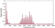
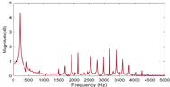
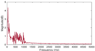
Based on the above formula, we can realize that the rotational Doppler shift is very sensitive to the detection conditions, and will produce different morphological distributions under different conditions. According to specific detection conditions, the common detected signal patterns can be divided into four categories as shown in Table 1. The corresponding features of frequency signals of the different categories are shown in the last column. Here, the frequency spectrum is generated under topological charge of ±12 and the rotational speed ranging from 10 to 100 round per second (rps). The only difference between each measurement is the relative pose between the axis of the rotating target and the detection beam.

Table 1.
Different categories of the RDE frequency signal.
It can be seen from Table 1 that when the beam axis is completely coaxial with the rotating axis, there will be only one frequency peak in the spectrum. When there is a lateral displacement between the two axes, the frequency peak will broaden into serval peaks. The interval between the peaks of these frequency signals is exactly the magnitude of the object’s rotating frequency, which is caused by the discrete nature of the beam OAM, as explained in detail in our previous article [29]. If the probe beam is obliquely illuminated at the rotating target, the frequency peal will broaden, too. But the interval between two peaks is larger than the last lateral condition. Finally, if the two axes are completely out of alignment, the signal will become a wide spectrum starting from zero.
In the real rotating speed measurement experiment, different signal extraction methods are required for each of the different signal characteristics mentioned above. The researcher needs to first identify the signal categories after spectral transformation and subsequently extract the rotating speed information from them according to the corresponding rules. This process can only be realized manually at present, and there is no automated method to achieve autonomous classification of the RDE signal. Therefore, if there is a way to realize the automatic identification of signal categories, the efficiency of rotating speed extraction can be effectively improved.
2.2. SVM Learning Model
SVM is a kind of binary classification model, and its basic model is a linear classifier with the largest margin defined on the feature space [27]. In simple terms, the support vector machine divides the training data into classes using a line or a surface in the space, and the principle is to maximize the margin. Here, the margin maximization refers to the maximum distance between the nearest point to the separating or surface in the feature space. Finding the hyperplane with the largest geometric margin on the training dataset means classifying the training data with a sufficiently high degree of certainty, and such a hyperplane has good classification and prediction capabilities for unknown new instances.
Based on the above definitions, the key factor in an SVM model is to find the best hyperplane through training. Since the dividing hyperplane is not certain, it is necessary to compare the distance from the same point to different hyperplanes. The distance from a point to a line in a two-dimensional space is as follows:
Extending the above two-dimensional plane distance formula to n-dimensional space, the distance from point to a hyperplane can be written as follows:
where .
In order to determine the optimal plane, combined with Equation (5) the mathematical model of the SVM regression prediction can be expressed as follows: [26]
where and are the parameters to be solved for the model. is the sample eigenvalues, and represents the sample label value.
Based on the above mathematical model, the SVM learning model can be constructed and trained according to the following steps. Firstly, the input and output parameters are determined. Here, each set of training data should contain topological charge, sampling rate and time-domine signal data, which are employed as training inputs. At the same time, the category of the set of signals is defined as the training output. Secondly, the core function is defined, which is used to map the sample data from a low-dimensional space to a high-dimensional space. Subsequently, the optimization model is defined according to Equations (6)–(9). The sequence minimum optimization algorithm is used here since it can quickly find the optimal solution while respecting linear constraints. Finally, determining the mode parameters. In an SVM learn model, there are two main parameters, i.e., penalty factor and core function factor . These two parameters are determined using heuristic methods, which can help the learning model achieve optimal prediction results.
3. Experimental Results
To verify the validity of the methods, we built the SVM learn model and trained it with the simulation datasets. The RDE simulation process is shown in Figure 1a. Firstly, based on the standard LG mode defined in Equation (1), the vortex beam is generated and then transmitted in free space for a certain distance using the ABCD matrix method. Subsequently, the probe beam illuminates the surface of the rotating object. Here, the rotating target is set as a flat rotating disc with a surface covered with reflective material. Then, the scattered light intensity is observed by directly multiplying the amplitude distribution of the vortex beam with the amplitude of the surface of the object , which can completely simulate the scattered light collection process in the experiment. Finally, the light intensity of the scattered light can be obtained based on the formula for the superposition of the light fields calculation.
where and . The third term in the above equation represents the coherent term of the two field. Given that the two fields lack coherence, the parameter in the third term is .
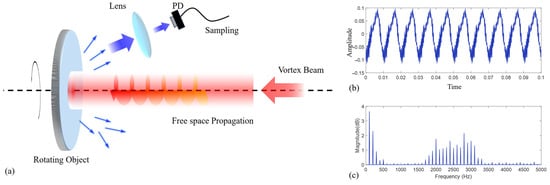
Figure 1.
Simulation process of the RDE detection. (a) The simulation process. The probe beam is transmitted through free space and then illuminated on the surface of the rotating target. Scattered light is then collected using lenses and photodetectors (PD), and time-domain signal data are obtained after scattering the sampling rate. (b) The time domain data. (c) The RDE frequency spectrum under small lateral displacement.
By correlating the rotational speed and time information, it is possible to sample the intensity of the scattered light at a certain moment with any sampling rate , and after setting a period of sampling time, the time-domain signal can be obtained. Here, the relationship between the angle through which an object rotates, and the sampling rate can be expressed as follows:
Figure 1b represents the result of the time domain signal obtained by sampling at a rate of 10,000 Hz. It can be seen that the light intensity fluctuates up and down around the value of zero being normalized. The RDE signal will manifest when a Fourier transform is performed on the data in the time domain. Figure 1c presents the RDE signal when there is a small lateral displacement between the probe beam and the rotating axis. It can be seen that the RDE signal shows a broadening pattern, which belongs to the second category.
Building upon the aforementioned simulation process, we will subsequently initiate the implementation of an adaptive signal classification method based on an SVM model. The first step is to prepare the training datasets used in the training model. One of the biggest advantages of the SVM-based machine learning model is that they do not require huge datasets. Table 2 presents the details of the dataset we generated by the simulation process. We collected a total of 800 sets of data. For each category, a total of 200 sets were collected at different speeds. Here, we use the numbers 1, 2, 3, and 4 to represent four different types of data. The topological charge of the detection beam used for each dataset is ±12. The rotational speed of the targets is set randomly, ranging from 10 rps to 110 rps.
Table 2.
Details of the training dataset.
Before the training process is started, the first step is to shuffle the order of the datasets. During the training process, we divide the dataset into training part and test part according to 8:2. In this experiment, there are only four categories of the signals, so the penalty factor can be set to a smaller value. Through experimental comparison, it is found that the ideal classification effect can be obtained when the penalty factor is 1500 and the radial basis function parameter is 0.0001. When the training result meets the optimal conditions, i.e., the reduction in the objective function between two consecutive iterations fell below the predefined epsilon value, the training automatically ends, and the model training result is output. As shown in Figure 2a,b, the categories of the test data are accurately determined and the corresponding accuracy of SVM model classification is as high as 100%.
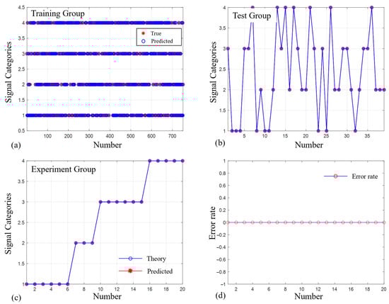
Figure 2.
The training and experimental results. (a,b) represent the results of SVM for the training and test group data, respectively. From the test data, the algorithm has achieved 100% accuracy in predicting the results for the signal categories. (c) Denotes the prediction of the learning model on the data of the experimental group. (d) shows the error rate curve. The predicted error rate for this dataset is zero. From the prediction results, it is accurate for the set of data with the same topological charges.
Based on the above-trained model, we carried out the verification based on the measured data. The corresponding experimental setups are similar to the simulation process. Detailed information about the device can be found in Refs. [29,31]. We collected 20 sets of probe data under topological charge of , and with a rotational speed ranging from 10 rps to 110 rps. For each distinct set of measured data, the trained model demonstrates the ability to classify the type of signal it represents accurately. The error rate of classification recognition is zero. To further verify the reliability of the classification model, we further carried out tests under different topological charges. This time, the data collection for the experimental set was conducted at different topological charges. The rotational speed was still from 10 rps to 110 rps, while the topological charges were taken as any integer value between and .
As is shown in Figure 3, we found that the accuracy of signal type identification decreases when the topological charges of the measurements are different. In this case, the accuracy of the model category predictions is 75%. This indicates that the generalization ability of the classification algorithm model needs to be strengthened. This result may also be due to the limited number of training datasets, and it is expected that a higher classification accuracy can be achieved by further increasing the training dataset in subsequent studies.
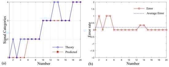
Figure 3.
Signal category prediction results for the detection data under different topological charges, ranging from to . (a) shows the comparison between theoretical values and predicted values, and (b) shows the corresponding prediction errors.
4. Conclusions
In this paper, we report a new method for RDE signal type recognition. With the help of the SVM learning model, we can accurately identify signal categories without FFT with high accuracy. Theoretically, based on the existing techniques, it is difficult to further improve the extraction accuracy of the target rotating speed associated with RDE from the improvement of the signal processing and the quality of the probe beam. At the same time, the use of machine learning is expected to provide a new way for high-precision signal type recognition and rotating speed detection under complex conditions. Experimentally, the learning model can realize the direct extraction of relative pose and rotation speed information of the target from the signals detected by the photodetector, which is more concise and efficient compared with manual computational identification. This approach also improves the degree of automation and is expected to be applied in engineering practice.
Author Contributions
Conceptualization, S.Q. and M.X.; methodology, S.Q.; software, S.Q.; validation, J.Z. investigation, J.Z.; writing—original draft preparation, S.Q.; writing—review and editing, S.Q.; supervision, J.Z. All authors have read and agreed to the published version of the manuscript.
Funding
This research was funded by National Nature and Science Foundation of China, grant number 62305007.
Institutional Review Board Statement
Not applicable.
Informed Consent Statement
Not applicable.
Data Availability Statement
All the data used in this article can be obtained from the author upon reasonable request.
Conflicts of Interest
The authors declare no conflicts of interest.
References
- Lavery, M.P.; Speirits, F.C.; Barnett, S.M.; Padgett, M.J. Detection of a spinning object using light’s orbital angular momentum. Science 2013, 341, 537–540. [Google Scholar] [CrossRef] [PubMed]
- Lavery, M.P.J.; Barnett, S.M.; Speirits, F.C.; Padgett, M.J. Observation of the rotational Doppler shift of a white-light, orbital-angular-momentum-carrying beam backscattered from a rotating body. Optica 2014, 1, 1–4. [Google Scholar] [CrossRef]
- Speirits, F.C.; Lavery, M.P.; Padgett, M.J.; Barnett, S.M. Optical angular momentum in a rotating frame. Opt. Lett. 2014, 39, 2944–2946. [Google Scholar] [CrossRef] [PubMed]
- Padgett, M. A new twist on the Doppler shift. Phys. Today 2014, 67, 58–59. [Google Scholar] [CrossRef]
- Phillips, D.B.; Lee, M.P.; Speirits, F.C.; Barnett, S.M.; Simpson, S.H.; Lavery, M.P.J.; Padgett, M.J.; Gibson, G.M. Rotational Doppler velocimetry to probe the angular velocity of spinning microparticles. Phys. Rev. A 2014, 90, 011801. [Google Scholar] [CrossRef]
- Singh, P.; Davuluri, S.; Rostovtsev, Y.V. Detection of Coriolis force and rotational Doppler effect by using slow light. Opt. Eng. 2014, 53, 102708. [Google Scholar] [CrossRef]
- Li, G.; Zentgraf, T.; Zhang, S. Rotational Doppler effect in nonlinear optics. Nat. Phys. 2016, 12, 736–740. [Google Scholar] [CrossRef]
- Rosales-Guzmán, C.; Hermosa, N.; Belmonte, A.; Torres, J.P. Measuring the translational and rotational velocities of particles in helical motion using structured light. Opt. Express 2014, 22, 16504–16509. [Google Scholar] [CrossRef]
- Cvijetic, N.; Milione, G.; Ip, E.; Wang, T. Detecting Lateral Motion using Light’s Orbital Angular Momentum. Sci. Rep. 2015, 5, 15422. [Google Scholar] [CrossRef]
- Cheng, T.-Y.; Wang, W.-Y.; Li, J.-S.; Guo, J.-X.; Liu, S.; Lü, J.-Q. Rotational Doppler Effect in Vortex Light and Its Applications for Detection of the Rotational Motion. Photonics 2022, 9, 441. [Google Scholar] [CrossRef]
- Hu, X.-B.; Zhao, B.; Zhu, Z.-H.; Gao, W.; Rosales-Guzmán, C. In situ detection of a cooperative target’s longitudinal and angular speed using structured light. Opt. Lett. 2019, 44, 3070–3073. [Google Scholar] [CrossRef] [PubMed]
- Emile, O.; Emile, J.; Brousseau, C. Rotational Doppler shift upon reflection from a right angle prism. Appl. Phys. Lett. 2020, 116, 221102. [Google Scholar] [CrossRef]
- Qiu, S.; Liu, T.; Li, Z.; Wang, C.; Ren, Y.; Shao, Q.; Xing, C. Influence of lateral misalignment on the optical rotational Doppler effect. Appl. Opt. 2019, 58, 2650–2655. [Google Scholar] [CrossRef] [PubMed]
- Qiu, S.; Liu, T.; Ren, Y.; Li, Z.; Wang, C.; Shao, Q. Detection of spinning objects at oblique light incidence using the optical rotational Doppler effect. Opt. Express 2019, 27, 24781–24792. [Google Scholar] [CrossRef] [PubMed]
- Deng, J.; Li, K.F.; Liu, W.; Li, G. Cascaded rotational Doppler effect. Opt. Lett. 2019, 44, 2346–2349. [Google Scholar] [CrossRef]
- Zhai, Y.; Fu, S.; Yin, C.; Zhou, H.; Gao, C. Detection of angular acceleration based on optical rotational Doppler effect. Opt. Express 2019, 27, 15518–15527. [Google Scholar] [CrossRef]
- Anderson, A.Q.; Strong, E.F.; Heffernan, B.M.; Siemens, M.E.; Rieker, G.B.; Gopinath, J.T. Detection technique effect on rotational Doppler measurements. Opt. Lett. 2020, 45, 2636–2639. [Google Scholar] [CrossRef]
- Qiu, S.; Ren, Y.; Liu, T.; Chen, L.; Wang, C.; Li, Z.; Shao, Q. Spinning object detection based on perfect optical vortex. Opt. Lasers Eng. 2019, 124, 105842. [Google Scholar] [CrossRef]
- Zhai, Y.; Fu, S.; Zhang, J.; Lv, Y.; Zhou, H.; Gao, C. Remote detection of a rotator based on rotational Doppler effect. Appl. Phys. Express 2020, 13, 022012. [Google Scholar] [CrossRef]
- Fang, L.; Wan, Z.; Forbes, A.; Wang, J. Vectorial Doppler metrology. Nat. Commun. 2021, 12, 4186. [Google Scholar] [CrossRef]
- Ding, Y.; Liu, T.; Qiu, S.; Liu, Z.; Sha, Q.; Ren, Y. Locating the center of rotation of a planar object using an optical vortex. Appl. Opt. 2022, 61, 3919–3923. [Google Scholar] [CrossRef] [PubMed]
- Anderson, A.Q.; Strong, E.F.; Heffernan, B.M.; Siemens, M.E.; Rieker, G.B.; Gopinath, J.T. Observation of the rotational Doppler shift with spatially incoherent light. Opt. Express 2021, 29, 4058–4066. [Google Scholar] [CrossRef] [PubMed]
- Larnimaa, S.; Vainio, M. Fourier-transform spectroscopy based on the rotational Doppler effect. AIP Adv. 2024, 14, 105329. [Google Scholar] [CrossRef]
- Vapnik, V.N. An overview of statistical learning theory. IEEE Trans. Neural Netw. 1999, 10, 988–999. [Google Scholar] [CrossRef]
- Krizhevsky, A.; Sutskever, I.; Hinton, G.E. Imagenet classification with deep convolutional neural networks. Commun. ACM 2017, 60, 84–90. [Google Scholar] [CrossRef]
- Chang, C.-C.; Lin, C.-J. LIBSVM: A library for support vector machines. ACM Trans. Intell. Syst. Technol. 2011, 2, 27. [Google Scholar] [CrossRef]
- Cortes, C.; Vapnik, V. Support-Vector Networks. Mach. Learn. 1995, 20, 273–297. [Google Scholar] [CrossRef]
- Qiu, S.; Liu, T.; Ding, Y.; Liu, Z.; Chen, L.; Ren, Y. Rotational Doppler Effect with Vortex Beams: Fundamental Mechanism and Technical Progress. Front. Phys. 2022, 10, 938593. [Google Scholar] [CrossRef]
- Qiu, S.; Ding, Y.; Liu, T.; Liu, Z.; Ren, Y. Rotational object detection at noncoaxial light incidence based on the rotational Doppler effect. Opt. Express 2022, 30, 20441–20450. [Google Scholar] [CrossRef]
- Allen, L.; Beijersbergen, M.W.; Spreeuw, R.J.C.; Woerdman, J.P. Orbital angular momentum of light and the transformation of Laguerre-Gaussian laser modes. Phys. Rev. A 1992, 45, 8185–8189. [Google Scholar] [CrossRef]
- Ren, Y.; Qiu, S.; Liu, T.; Liu, Z.; Cai, W. Non-Contact Ultralow Rotational Speed Measurement of Real Objects Based on Rotational Doppler Velocimetry. IEEE Trans. Instrum. Meas. 2022, 71, 1–8. [Google Scholar] [CrossRef]


Disclaimer/Publisher’s Note: The statements, opinions and data contained in all publications are solely those of the individual author(s) and contributor(s) and not of MDPI and/or the editor(s). MDPI and/or the editor(s) disclaim responsibility for any injury to people or property resulting from any ideas, methods, instructions or products referred to in the content. |
© 2025 by the authors. Licensee MDPI, Basel, Switzerland. This article is an open access article distributed under the terms and conditions of the Creative Commons Attribution (CC BY) license (https://creativecommons.org/licenses/by/4.0/).