A Vibration Signal Detection System Based on Double Intensity Modulation

Abstract

The measurement system proposed in this paper, based on double intensity modulation, can achieve the detection and recovery of vibration signals. The system uses a Mach–Zehnder modulator to modulate the intensity of the laser light before and after it is reflected from the target, and the modulated optical signal carries the vibration signal information. After photoelectric conversion and data processing, the system measures and recovers the amplitude and frequency of the vibration signal. For sinusoidal signals, amplitudes of $15\mathsf{\mu }$m, $25\mathsf{\mu }$m and $40\mathsf{\mu }$m and frequencies of 100 Hz, 500 Hz and 1000 Hz were measured, and the experimental results demonstrate that the rapid measurement and waveform recovery of such signals can be achieved using our proposed system. Specifically, the absolute deviation in amplitude measurement is less than $0.13\mathsf{\mu }$m, and the relative error does not exceed 0.35%; the absolute deviation in frequency measurement is less than 0.35 Hz, with a relative error below 0.01%; and a refresh rate of up to 4 kHz can be reached. Moreover, an aluminum plate is selected as the target object instead of the reflector in the system, providing a new method for vibration signal detection and expanding the scope of dynamic detection in industrial applications.

1. Introduction

With the rapid development of aerospace, precision instruments, chip manufacturing and other technologies, the demand for high-precision, high-stability vibration signal detection systems is becoming increasingly pronounced. For example, during spacecraft missions, accurately measuring sources of micro-vibration perturbation is necessary for obtaining accurate feedback data to ensure smooth spacecraft operation [1,2]. In microelectromechanical systems and precision computing, it is necessary to obtain physical quantities, such as acceleration, indirectly through high-precision measurement of vibration signals, and the measurement accuracy directly determines the accuracy of subsequently measured physical quantities [3,4]. In mechanical equipment monitoring, it is necessary to use technology for the detection of tiny vibration signals in monitoring the operating status of the equipment in real time to prevent the occurrence of failures [5,6]. In chip manufacturing, chip integration density is continuously increasing. Consequently, a chip of the same size must accommodate more electronic components. This necessitates high-precision tiny vibration measurement and feedback control of photolithography on silicon wafers to ensure the precision and consistency of process steps, such as photoresist application, development, and etching [7]. It can be seen that high-precision, high-stability vibration signal measurement technology has broad market demand and application prospects.

At present, vibration signal measurement technologies are mainly categorized as non-optical and optical measurement technologies [8,9], of which non-optical technologies mostly encompass mechanical and electrical measurement. Typical representative methods include piezoelectric sensors based on the piezoelectric effect, in which the vibration acceleration is characterized based on the change in charge, and capacitive sensors based on capacitance, in which the change in capacitance caused by the change in distance between the plates is used to derive the vibration signal detection function. However, mechanical measurements are mostly contact measurements, with limited applications [10,11,12], whereas electrical measurements are susceptible to electromagnetic field interference. Optical measurement technologies have the advantages of high accuracy, non-contact measurement and anti-electromagnetic interference, and have received wide attention worldwide.

In 2019, Li Jiaqi et al. designed a vibration signal measurement system based on the laser triangulation method [13]. In this system, a semiconductor laser is modulated by a drive circuit, and the modulated laser beam is collimated by a lens and then irradiated onto the surface of the object to be measured. Scattered light from the measured surface is then projected onto the photosensitive surface of the photoelectric position sensor PSD (position sensitive detector) by the imaging lens. The displacement value is derived from the PSD signal output, which undergoes analog-to-digital conversion and data processing. The experimental results show that the system can achieve a measurement range of up to 20 mm with an accuracy of $24\mathsf{\mu }$m. However, as the measurement range is extended, the size of the laser spot increases accordingly, resulting in a decrease in measurement accuracy.

In 2024, Pan Wen et al. proposed a measurement system based on fiber optic Mach–Zehnder interference [14], in which a photodetector is used to measure displacement information from interference between modulated reference light and measurement light. In signal demodulation, the correlation forensic method, which can judge whether the signal phase is ahead or behind, is used to obtain the magnitude and direction of the vibration displacement. Although the system achieves a maximum relative error of 0.78% in vibration displacement measurement over a range of $\pm 25\mathsf{\mu }$m, the system requires high-precision optics and is susceptible to environmental vibration, limiting its applicability.

In 2025, Jia Peng et al. from Zhejiang University of Technology developed a fiber optic interferometric vibration measurement system based on internal modulation [15]. To measure the vibration source, the system internally modulates the current of a DFB (distributed feedback) laser and outputs the measurement light through a fiber ring surface and a fiber microprobe, and the returned measurement light then interferes with the self-reflected reference light of the fiber microprobe. The system achieves high-precision measurement of vibration displacement with a vibration frequency range of 1142 Hz; the average deviation in measurement of $0.173\mathsf{\mu }$m is determined in a $10\mathsf{\mu }$m displacement step experiment, the resolution of vibration frequency is 1.221 Hz, and the harmonic distortion rate is less than 1.36%. However, the internal modulation introduces nonlinear errors that must be compensated for in the vibration signal resolution, increasing the complexity of the system design.

In summary, in the field of vibration signal measurement, mechanical measurement is based on simple structures and is low cost but mostly encompasses contact measurement, in which interference to the measured system readily arises; electrical measurement has been proposed for avoiding the above problems and, at the same time, demonstrates excellent performance in high-frequency response and has high sensitivity. However, due to the characteristics of piezoelectric materials, there are problems of temperature drift and external electromagnetic interference. In contrast, optical measurement does not depend on contact with the target nor have the disadvantages of electromagnetic interference, and it has the advantages of high measurement accuracy and speed [16,17,18,19]. However, at present, optical measurement technology also has the disadvantages of nonlinear error, difficulty in adjusting the optical path and high system complexity. Therefore, it is worth exploring the development of a vibration signal detection system based on the optical principle that has high measurement accuracy, a wide application range and a simple system structure.

In this paper, a vibration signal detection system based on double modulation is proposed. The MZM (Mach–Zehnder modulator) sequentially modulates the intensity of the pre- and post-reflected optical signals, avoiding the phase nonlinear error generated by the internal modulation; the optical signals carrying the vibration information after secondary modulation are acquired via photoelectric conversion, through which it is possible to measure and recover the vibration information using the Fourier transform algorithm. The theoretical range of the system can reach up to 1 mm, based on the performance limitations of piezoelectric ceramics, the actual range is as high as $40\mathsf{\mu }$m, and the frequency range covers 1000 Hz. In the amplitude measurement experiments of $15\mathsf{\mu }$m, $25\mathsf{\mu }$m and $40\mathsf{\mu }$m, the absolute deviation in the vibration displacement detection results is less than $0.12\mathsf{\mu }$m, and the relative error does not exceed 0.35%. In the frequency measurement experiments of 100 Hz, 500 Hz and 1000 Hz, the absolute deviation in the vibration frequency detection results does not exceed 0.35 Hz, and the relative error does not exceed 0.01%. With the simple measurement structure and the choice of aluminum plate as the target instead of the reflector in the traditional measurement system, the system represents a new method for detecting vibration signals, which is expected to be applied to precision vibration detection in industrial fields.

2. System Principle

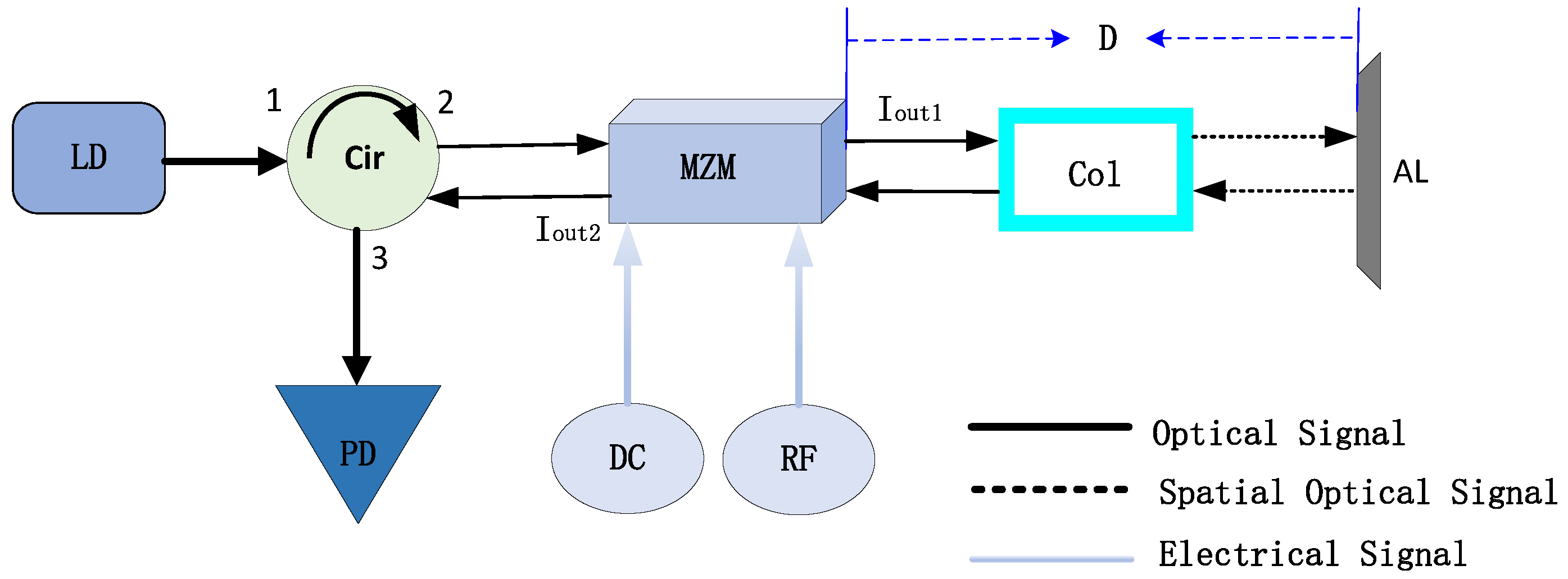
2.1. Double Modulation Principle

The principle of the double modulation system proposed in this paper is shown in Figure 1.

The optical signal outputs from the laser and enters port 1 of the Cir, and then outputs from port 2 of the Cir and enters the MZM, at which time the MZM performs the first intensity modulation on the optical signal. In this system, it is assumed that the input optical signal is

$$A_i\left(t\right)=A_{0}exp\left(i{\omega }_{0}t\right)$$

(1)

where $A_0$ is the input optical signal intensity, and ${\omega }_0$ is the input optical signal angular frequency. According to the transfer function of the MZM [20,21], the modulated output signal light intensity can be expressed as follows:

$$I_{out1}={\displaystyle \frac{1}{2}}{I}_{in}(1+cos(\Delta \varphi 1))$$

(2)

$$\Delta \varphi 1=\pi {\displaystyle \frac{V_d+V_{a}cos\left({\omega }_{a}t\right)}{V_{\pi }}}$$

(3)

where $I_{in}$ is the light intensity of the input optical signal, $I_{in}=A_0^2$; $\Delta \varphi 1$ is the phase shift generated after the first modulation; $V_d$ represents the external DC bias voltage loaded on the modulator; $V_a$ represents the voltage amplitude of the loaded RF signal; ${\omega }_a$ represents the angular frequency of the RF signal; $V_{\pi }$ represents the forward half-wave voltage. The first modulated optical signal enters the collimator, which outputs free-space light that is reflected by the target and then returns to the MZM for the second intensity modulation, and the modulated intensity is expressed as follows:

$$\begin{array}{cc}\hfill I_{out2}& ={\displaystyle \frac{1}{4}}{I}_{in}(1+cos\Delta \varphi 1)(1+cos(\Delta \varphi 2))\hfill \\ \hfill & ={\displaystyle \frac{1}{4}}{I}_{in}[cos(\Delta \varphi 1)cos(\Delta \varphi 2)+cos(\Delta \varphi 1)+cos(\Delta \varphi 2)+1]\hfill \end{array}$$

(4)

$$\Delta \varphi 2=\pi {\displaystyle \frac{V_d+V_{a}cos\left[{\omega }_a(t+\Delta t)\right]}{V_{\pi }^{\prime }}}$$

(5)

where $\Delta \varphi 2$ is the phase shift generated after the second modulation; $\Delta t$ is the time-of-flight of the optical signal, defined as the time interval between the first modulated optical signal being output from the MZM output, being reflected by the target, and entering the MZM again; $V_{\pi }^{\prime }$ is the reverse half-wave voltage.

Depending on the external DC bias voltage, the MZM has three operating states: maximum transmission point, minimum transmission point and quadrature transmission point [22,23,24]. When the MZM operates in the quadrature transmission point, it is most sensitive to the interference effect of the two internal optical signals, and the phase difference between the two optical signals is an odd multiple of ${\displaystyle \frac{1}{2}}\pi$ [25,26]. Based on this, the MZM works at the quadrature transmission point in this study, $V_d={\displaystyle \frac{3}{2}}V\pi$. And introducing Equations (3) and (5), combined with the first-order Bessel function [27,28], it is expanded for $cos(\Delta \varphi 1)$ and $cos(\Delta \varphi 2)$, where only the first-order term is retained, resulting in the following:

$$\cos (\Delta \varphi 1)=2J_1\left(k\right)cos\left({\omega }_{a}t\right)$$

(6)

$$\cos (\Delta \varphi 2)=2J_1\left(k^{\prime }\right)cos\left[{\omega }_a(t+\Delta t)\right]$$

(7)

Introducing Equations (6) and (7) into Equation (4), we obtain

$$\begin{array}{cc}\hfill I_{out2}={\displaystyle \frac{1}{4}}{I}_{in}& \{2J_1\left(k\right)J_1\left(k^{\prime }\right)\cos ({\omega }_a\Delta t)+2J_1\left(k\right)J_1\left(k^{\prime }\right)\cos \left[{\omega }_a(t+\Delta t)\right]\\ & +2J_1\left(k\right)\cos \left({\omega }_{a}t\right)+2J_1\left(k^{\prime }\right)\cos \left[{\omega }_a(t+\Delta t)\right]+1\}\end{array}$$

(8)

where $k={\displaystyle \frac{\pi V_a}{V_{\pi }}}$ denotes the forward modulation depth of the modulator; $k^{\prime }={\displaystyle \frac{\pi V_a}{V_{\pi }^{\prime }}}$ denotes the reverse modulation depth of the modulator. The half-wave voltage parameter $V_{\pi }$ of the MZM selected in the experiment is 6 V, the amplitude $V_a$ of the applied RF signal is 0.6 V, which gives the modulation depth k of MZM to be about 0.314. The forward and reverse modulation depths are treated as equivalent values in the study. At this point, the coefficient of the first order term of the Bessel function is 0.15 and the coefficient of the third order term is 0.0006. When the target is stationary, $\Delta t$ remains constant, and $cos({\omega }_a\Delta t)$ is a fixed value representing the DC component. When the bandwidth of the PD, on the order of kilohertz (kHz), is significantly smaller than ${\omega }_a$, on the order of gigahertz (GHz), only the DC component of the output signal is retained, and the power expression of the output optical signal after double modulation is obtained:

$$I_{out2}={\displaystyle \frac{1}{4}}{I}_{in}[1+2J_1\left(k\right)J_1\left(k^{\prime }\right)cos({\omega }_a\Delta t)]$$

(9)

$I_{out2}$ satisfies a cosine function with ${\omega }_a$ and $\Delta t$, which will be used in subsequently calculating the displacement of the signal to be measured.

2.2. Vibration Signal Detection Principle

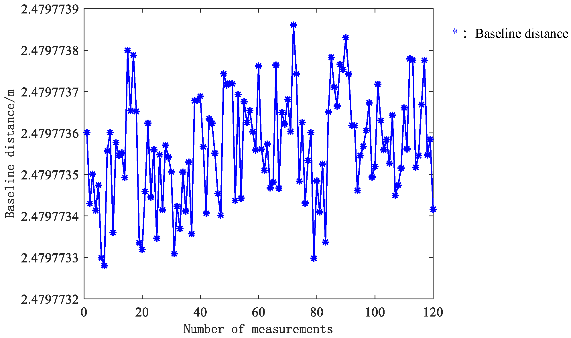
2.2.1. Obtaining the Baseline Distance

Assume D is the baseline distance, denoting the distance from the MZM output to the target; c is the speed of light in vacuum; n is the equivalent refractive index of air; and $f_a$ is the modulating signal frequency, where ${\omega }_a=2\pi f_a$. Then, the flight time can be expressed as:

$$\Delta t={\displaystyle \frac{2Dn}{c}}$$

(10)

Introducing Equation (10) into Equation (9) gives:

$$I_{out2}\propto \cos \left({\displaystyle \frac{4\pi f_{a}Dn}{c}}\right)$$

(11)

It can be seen that there is a cosine function relationship between $I_{out2}$ and $f_a$, and the phase difference between two adjacent minima is $2\pi$. In this paper, the modulation frequency of the MZM is changed by sweeping, and we obtain the modulation frequency values corresponding to the two adjacent power minima, which are written as $f_1$ and $f_2$, and the corresponding phases are written as $(2N-1)\pi$ and $(2N+1)\pi$, which can be obtained as follows:

$${\displaystyle \frac{4\pi f_{1}Dn}{c}}=(2N-1)\pi$$

(12)

$${\displaystyle \frac{4\pi f_{2}Dn}{c}}=(2N+1)\pi$$

(13)

where N is a positive integer. The expression for $2N-1$ can be obtained by associating Equations (12) and (13):

$$2N-1={\displaystyle \frac{2f_1}{f_2-f_1}}$$

(14)

This leads to the expression for D:

$$D=(2N-1){\displaystyle \frac{c}{4n{f}_1}}=\left[{\displaystyle \frac{2f_1}{f_2-f_1}}\right]{\displaystyle \frac{c}{4n{f}_1}}$$

(15)

[ ] denotes the rounding operation. According to Equation (15), it can be seen that D can only be found by first determining $f_1$ and $f_2$, and next we will examine how to accurately obtain $f_1$ and $f_2$.

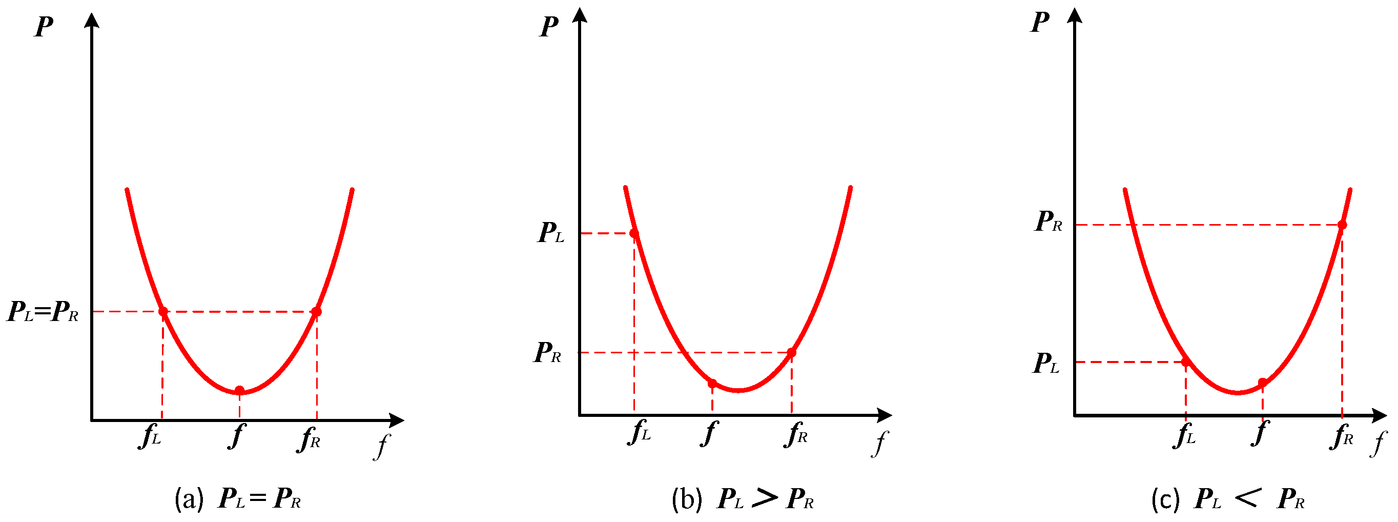
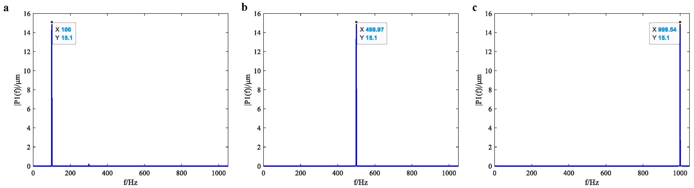
2.2.2. Obtaining Frequency Values by Swing Fitting

In the traditional method, direct measurement is used to obtain the desired frequency value [29,30]. Multiple frequency scans are performed from the frequency starting point, resulting in a long processing time. The value set for the scanning step value directly affects the accuracy of the frequency value. To improve the measurement speed and data accuracy, we propose using an indirect measurement method, the swing fitting method, to obtain the desired modulation frequency value, and the basic principle is shown in Figure 2.

Illustrated here is the example of obtaining $f_1$, assuming that the frequency offset is $\delta f$. In Figure 2, f is defined as the center frequency. The decrease in f by $\delta f$ is denoted as $f_L$, and the increase in f by $\delta f$ is denoted as $f_R$. Due to the symmetry of the cosine function, when $f=f_1$, the power values of the signals corresponding to $f_L$ and $f_R$, which are denoted as $P_L=P_R$, are equal, as shown in Figure 2a; and when $f\ne f_1$, the power values of the output signals corresponding to $f_L$ and $f_R$ are unequal. Then, $P_L\ne P_R$, as shown in Figure 2b,c. The difference between $P_L$ and $P_R$ is denoted as $\Delta P$, and $\Delta P$ is expressed by the Equation (16):

$$\Delta P=-I_{in}{J}_1\left(k\right)J_1\left(k^{\prime }\right)sin\left({\displaystyle \frac{4\pi \left(\delta f\right)Dn}{c}}\right)sin\left({\displaystyle \frac{4\pi fDn}{c}}\right)$$

(16)

Assuming that $\delta f$ remains constant, $a=-I_{in}{J}_1\left(k\right)J_1\left(k^{\prime }\right)sin\left({\displaystyle \frac{4\pi fDn}{c}}\right)$. Thus, a is a fixed value, and it can be obtained by substituting a into Equation (16):

$$\Delta P=asin\left({\displaystyle \frac{4\pi \left(\delta f\right)Dn}{c}}\right)$$

(17)

There is a sinusoidal functional relationship between $\Delta P$ and f. The curve near $\Delta P=0$ can be approximated as a primary function, and the corresponding function curve is shown in Figure 3.

When the modulation frequency changes from $f_L$ to $f_R$, $\Delta P$ also changes from a positive to a negative value and contains the point where $\Delta P=0$. This represents the intersection of the primary function and the transverse axis, and $f_1$ is the value of the transverse coordinate of the intersection point. $f_L$ and $f_R$ corresponding to $\Delta P$ are written as $\Delta P_L$ and $\Delta P_R$, which can be obtained according to the principle of triangle similarity:

$${\displaystyle \frac{f_1-f_L}{f_R-f_1}}=\left|{\displaystyle \frac{\Delta P_L}{\Delta P_R}}\right|$$

(18)

Simplification of the above equation gives:

$$f_1=f_L+{\displaystyle \frac{f_R-f_L}{1-\frac{\Delta P_R}{\Delta P_L}}}$$

(19)

By directly measuring $\Delta P$, the small change in $f_1$ is amplified, and $f_1$ is indirectly acquired, which effectively improves the sensitivity of the system to extract data and reduces the measurement error.

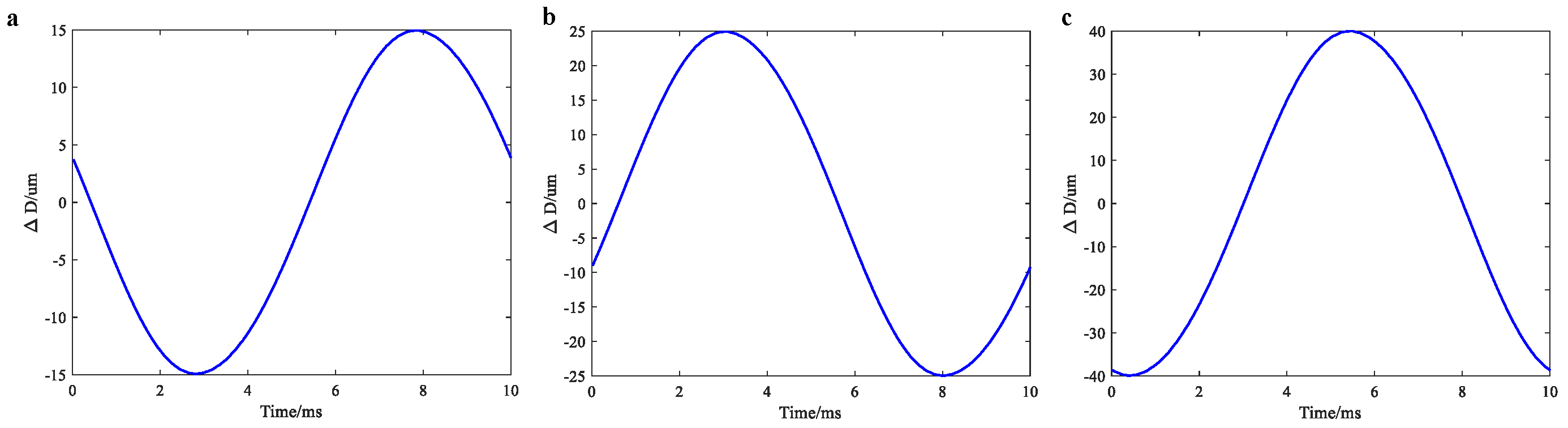
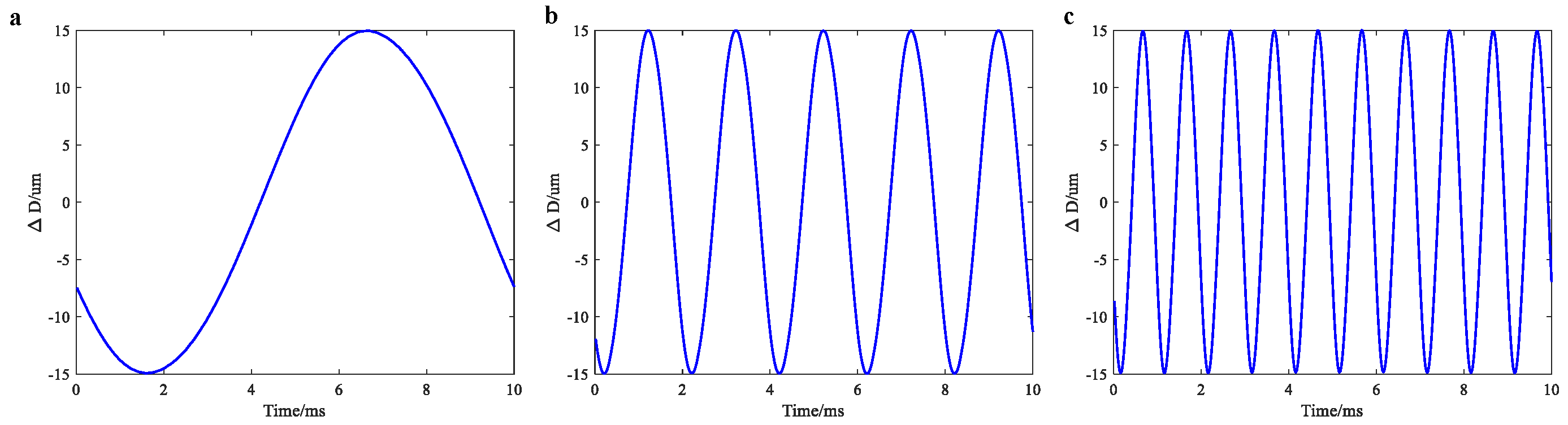
2.2.3. Vibration Displacement Measurement

When the target is subjected to external force to produce a small vibration, the baseline distance D will undergo a small change, and the changed distance is recorded as $(D+\Delta D)$. Analyzing Equation (12), the right side of the equation remains unchanged, which produces an offset in the modulation frequency $f_1$ corresponding to the first point of light intensity minima such that the equation remains in balance, and the value after the offset is noted as $f_1^{\prime }$, which then gives:

$${\displaystyle \frac{4\pi f_1^{\prime }(D+\Delta D)n}{c}}=(2N-1)\pi$$

(20)

The association of Equations (12) and (20) results in:

$$\Delta D={\displaystyle \frac{f_1-f_1^{\prime }}{f_1}}$$

(21)

The value of vibration displacement $\Delta D$ can be calculated according to Equation (20), and the direction of vibration displacement can be judged according to the positive or negative of $\Delta D$. In the experiment, using the swing fitting method, only two frequency scans are needed to measure $\Delta P_L$ and $\Delta P_R$ and then obtain $f_1$, and the value of $f_1^{\prime }$ can be obtained using the same method. Compared with the method of directly measuring the frequency corresponding to the point of light intensity minima, the swing method has a significant advantage in reducing the number of frequency hops, and the vibration signal displacement value can be obtained at once by performing four frequency scans, which significantly improves the measurement speed. Using the measurement system proposed in this paper, combined with the swing fitting algorithm, an update rate of up to 4 kHz/s for vibration displacement can be reached.

2.3. Analysis of the Vibration Displacement Range

Bring Equation (14) into Equation (12) and simplify:

$$D={\displaystyle \frac{c}{2n(f_2-f_1)}}$$

(22)

The target produces a small vibration, and $f_1$ occurs to shift the frequency, defining the difference between $f_1$ and $f_1^{\prime }$ as the frequency deviation as $\Delta f$, where $\Delta f<(f_2-f_1)$. According to Equation (21), D is inversely proportional to $(f_2-f_1)$, so the smaller D is, the larger $(f_2-f_1)$ is, and thus the larger $\Delta f$ is, and the larger $\Delta D$ is.

It can be seen that when measuring the baseline distance, increasing the modulation frequency is conducive to improving system accuracy [31]. Analyzing Equation (21), the larger $f_1$ is, the smaller $\Delta D$ is when $\Delta f$ is unchanged. Taking the system range into account, the modulation frequency cannot be infinitely large. For range design, the system measurement accuracy and the actual measurement situation should be considered, assuming that the baseline distance of the system is 2 m, the modulation frequency $f_1$ is 10 GHz, and the vibration displacement measurement range is 1 mm. In the present system, the maximum vibration displacement that can be measured in experiments is $40\mathsf{\mu }$m, due to limitations resulting from the maximum range of the piezoelectric ceramics that are used.

3. Experiment System Setup

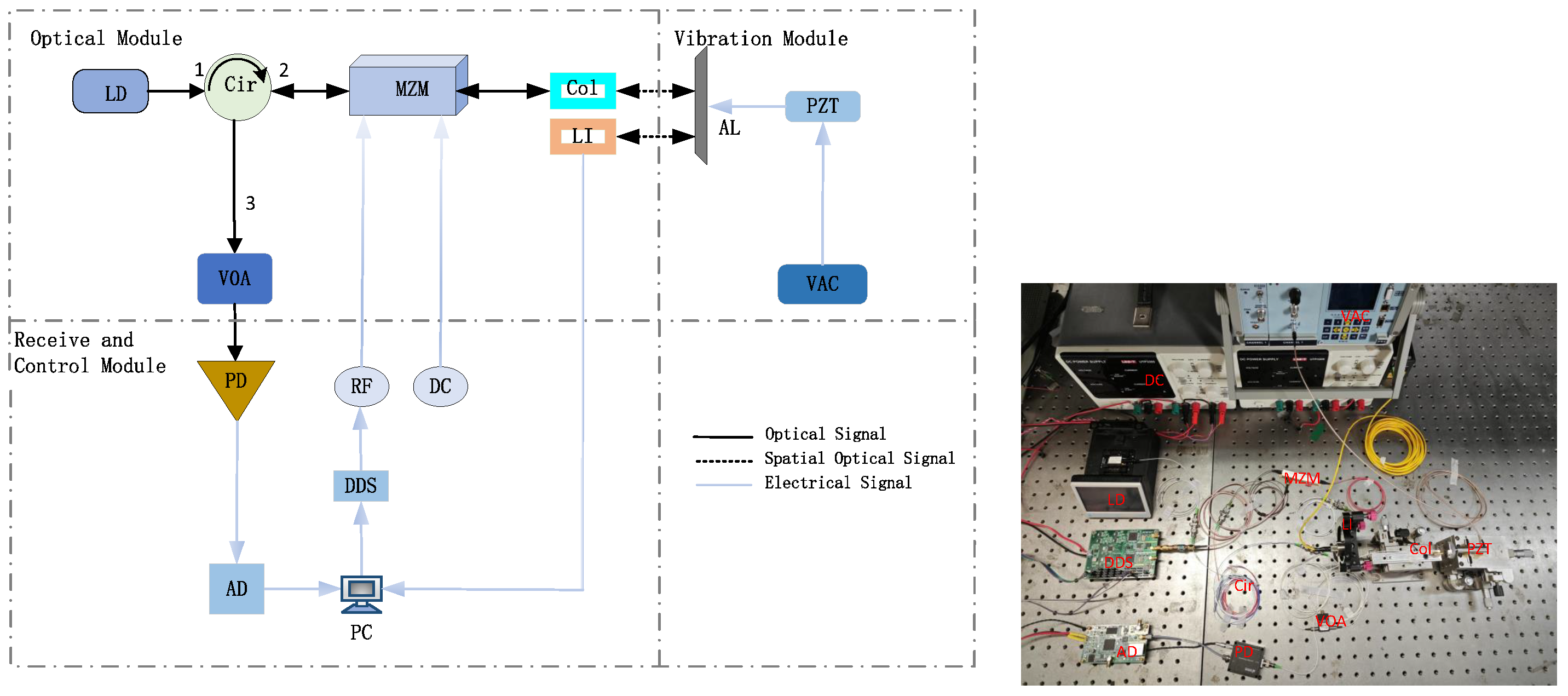
3.1. Hardware System Setup

According to the experimental principle, the experimental setup is built as shown in Figure 4. The experimental setup contains three modules: optical, vibration, and receive and control.

The optical module consists of the following devices: distributed feedback semiconductor laser (laser device, LD), center wavelength of $\lambda$ = 1550 nm, output power of 15 dBm; circulator (Cir), insertion loss of 0.7 dB; Mach–Zehnder modulator (MZM, center wavelength of $\lambda$ = 1550 nm); collimator (Col), outgoing loss of 0.5 dB; variable optical attenuator (VOA), adjustable attenuation range of 0.8–60.0 dB; laser interferometer (LI), Attocube Systems IDS3010 model, with a resolution of 1 pm. The optical module completes the laser emission and modulation function: the LD emission laser enters circulator port 1, through the circulator port 2, into the MZM to complete the first modulation, and the modulated laser that enters the fiber optic collimator is converted to free-space light, reflected by the aluminum plate back into the collimator, again into fiber optic light signals, and then into the MZM for the second modulation. After the modulation is completed, the optical signal enters the VOA for power adjustment. In the vibration signal measurement, the laser interferometer acquires data at the same time, performs calculation on the data to produce a reference, and subsequently compares and analyzes this with the experimental results.

The vibration module consists of a smooth-surface aluminum plate (Al), with dimensions of 10 mm × 10 mm × 3 mm; piezoelectric ceramics (PZT), with a nominal stroke of 0–40 $\mathsf{\mu }$m; voltage amplifier controller (VAC), with an analog input range of 0–10 V, output voltage range of 0–120 V, and output voltage resolution of 1/30,000. The module completes vibration signal generation and transmission in the piezoelectric ceramic connected to a smooth aluminum plate. The control of the VAC drives the PZT, whereas the aluminum plate produces a regular small vibration. The collimated free-space light arrives at the aluminum plate and is reflected, carrying the vibration information, to return along the original path.

The receive and control module includes a photoelectric detector (PD), response bandwidth of 10 kHz, saturated optical power of $2\mathsf{\mu }$W; analog-to-digital-converter data acquisition card (AD); direct digital frequency synthesis (DDS); personal computer (PC); direct current power supply (DC). The received optical signals sequentially enter the PD and AD to complete photoelectric conversion and analog-to-digital conversion. On the one hand, the PC receives and processes the data. On the other hand, it controls the DDS to generate the RF signal, which is used as the signal source to provide an AC drive for the MZM, and the DC provides external DC bias for the MZM to function at the orthogonal transmission point.

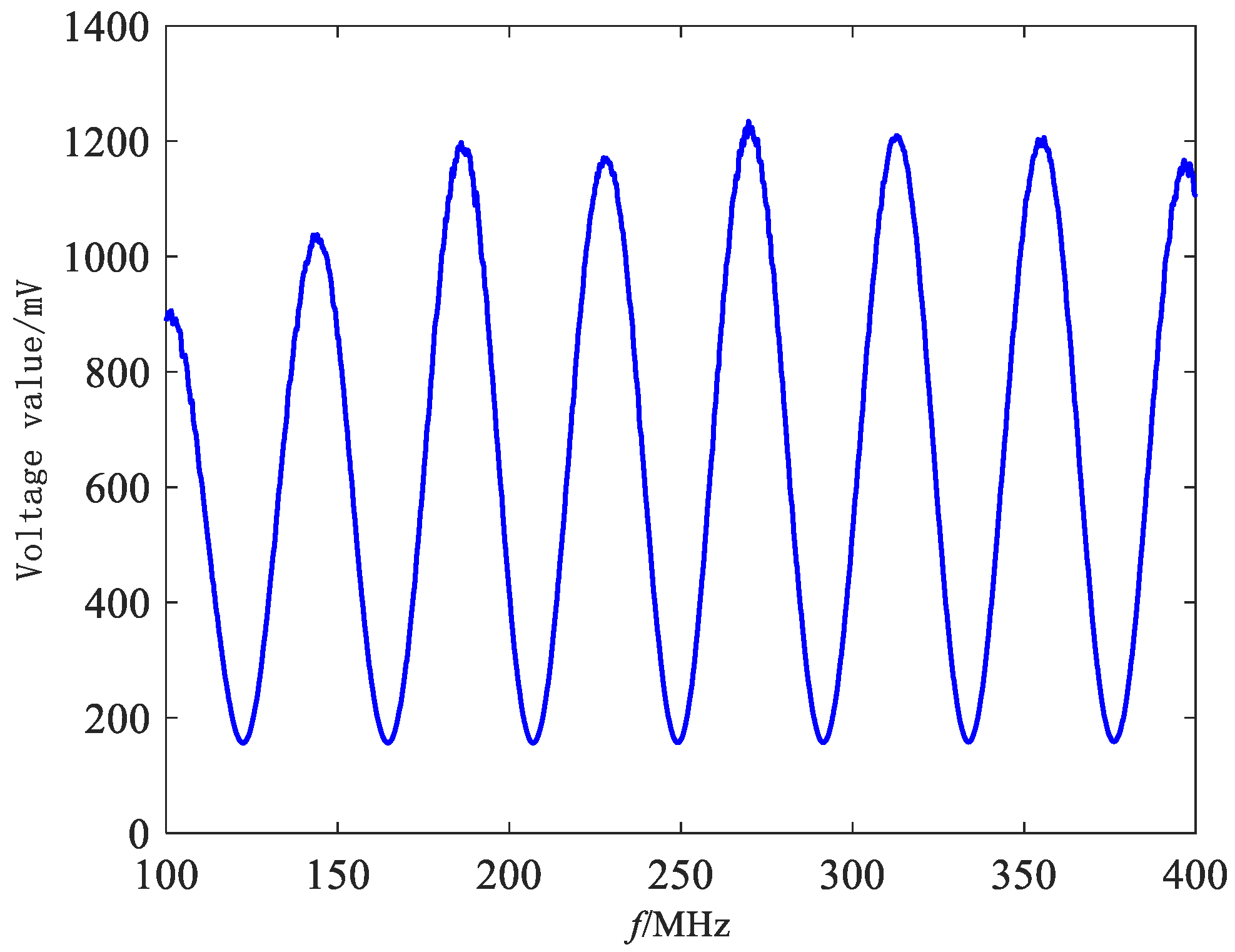
3.2. Sweep Curve Measurement

After completion of the experimental system, the frequency sweep curve is measured. The parameters in the experiment are set as follows: the signal waveform is sinusoidal, the frequency sweep range is 100–400 MHz, and the frequency sweep step value is 1 kHz. The results from plotting the data collected by the AD through the computer are shown in Figure 5, in which the horizontal axis denotes the modulation frequency, and the vertical axis denotes the value of the voltage detected by the PD.

The results of the frequency sweep curves demonstrate that the PD output power has a cosine relationship with the modulation frequency, which is consistent with the derivation of Equation (11), verifying the correctness of the theoretical derivation and providing the support for the measurement of vibration displacement.

4. Experimental Results and Analysis

4.1. Baseline Distance Measurement Results

In experiments, the baseline distance is measured by keeping the aluminum plate stable and repeating the measurement 120 times in the same measurement environment, and the experimental results are plotted as shown in Figure 6, where the horizontal axis indicates the number of measurements and the vertical axis indicates the baseline distance.

Analyzing Figure 6, it can be seen that from the 120 measurements, the baseline distance is stable at 2.47 m, and the range of fluctuation does not exceed $0.58\mathsf{\mu }$m; from further calculations based on the above data, we can determine that the average value is 2.4797736 m, the standard deviation is $0.13\mathsf{\mu }$m, and the system’s relative ranging accuracy is $2.3\times {10}^{-7}$. To reduce the error, the average of all measurements is taken as the baseline distance.

4.2. Vibration Signal Measurement Results

4.2.1. Laser Interferometer Measurement Results

The software is used to set the parameters of the VAC and drive the PZT to the aluminum plate for the force, causing the aluminum plate to produce a small vibration. The vibration signal frequency is set to 100 Hz, and the vibration amplitude is set to $15\mathsf{\mu }$m, $25\mathsf{\mu }$m and $40\mathsf{\mu }$m. The displacement value of the vibration system is measured using a laser interferometer, and the measurement results are shown in Figure 7 and Figure 8.

In Figure 7, the horizontal axis indicates the measurement time and the vertical axis indicates the vibration displacement. Figure 7a–c show the time domain measurement results of the sine wave signal with a vibration frequency of 100 Hz and vibration amplitudes of $15\mathsf{\mu }$m, $25\mathsf{\mu }$m and $40\mathsf{\mu }$m, respectively. In Figure 8, the horizontal axis indicates the frequency of the vibration signal, and the vertical axis indicates the amplitude of the vibration signal. Figure 8a–c show the frequency domain measurement results of the sine wave signals with a vibration frequency of 100 Hz and vibration amplitudes of $15\mathsf{\mu }$m, $25\mathsf{\mu }$m and $40\mathsf{\mu }$m, respectively. For the amplitudes of $15\mathsf{\mu }$m, $25\mathsf{\mu }$m and $40\mathsf{\mu }$m, the laser interferometer measurement results are $15.0001\mathsf{\mu }$m, $25.0002\mathsf{\mu }$m and $40.0001\mathsf{\mu }$m.

The vibration signal amplitude is set to $15\mathsf{\mu }$m, and the vibration frequency is set to 100 Hz, 500 Hz and 1000 Hz. The frequency values of the vibration system are measured using a laser interferometer, and the measurement results are shown in Figure 9 and Figure 10.

In Figure 9, the horizontal axis indicates the measurement time, and the vertical axis indicates the vibration displacement. Figure 9a–c show the time domain measurement results of the sinusoidal signals with a vibration amplitude of $15\mathsf{\mu }$m and vibration frequencies of 100 Hz, 500 Hz and 1000 Hz, respectively. In Figure 10, the horizontal axis indicates the frequency of the vibration signal, and the vertical axis indicates the amplitude of the vibration signal. Figure 10a–c show the frequency domain measurement results of the sine wave signals with a vibration amplitude of $15\mathsf{\mu }$m and vibration frequencies of 100 Hz, 500 Hz and 1000 Hz, respectively. For frequencies of 100 Hz, 500 Hz, and 1000 Hz, the laser interferometer measurement results are 100 Hz, 500 Hz and 1000 Hz. The above amplitude and frequency measurement results will be subsequently used as reference data for comparing and analyzing the experimental system measurement results.

4.2.2. Measurement Results of Experimental System

The sine wave signals with different amplitudes and frequencies were measured using the experimental system, and the data collected for 10 ms were processed using the computer. In this paper, the data is collected using an AD and then transferred to a computer via a network cable. Then, we use the computer program to calculate the vibration displacement and Fourier transform to get the vibration displacement and vibration frequency, and finally we make a plot of the measurement results. The specific results are shown in Figure 11, Figure 12, Figure 13, Figure 14, Figure 15 and Figure 16.

Figure 11a–c show the time domain measurement results of the sine wave signal with an amplitude of $15\mathsf{\mu }$m and frequencies of 100 Hz, 500 Hz and 1000 Hz, respectively, where the horizontal axis indicates the measurement time in milliseconds(ms), and the vertical axis indicates the vibration displacement in micrometers ($\mathsf{\mu }$m). Figure 12 shows the frequency domain measurement results corresponding to the above sinusoidal signals, where the horizontal axis indicates the frequency recovery result of the vibration signals, and the vertical axis represents the amplitude recovery result of the vibration signal.

Figure 13a–c show the time domain measurement results of a sine wave signal with an amplitude of $25\mathsf{\mu }$m and frequencies of 100 Hz, 500 Hz and 1000 Hz, respectively, where the horizontal axis indicates the measurement time in milliseconds (ms), and the vertical axis indicates the vibration displacement in micrometers ($\mathsf{\mu }$m). Figure 14 shows the frequency domain measurement results corresponding to the above sine wave signal, where the horizontal axis indicates the frequency restoration results of the vibration signal, the vertical axis represents the amplitude recovery result of the vibration signal.

Figure 15a–c show the time domain measurement results of the sine wave signals with amplitude of $40\mathsf{\mu }$m and frequencies of 100 Hz, 500 Hz and 1000 Hz, respectively, where the horizontal axis indicates the measurement time in milliseconds (ms), and the vertical axis indicates the vibration displacement in micrometers ($\mathsf{\mu }$m). Figure 16 shows the frequency domain measurement results corresponding to the above sine wave signals, where the horizontal axis indicates the frequency recovery result of the vibration signals, and the vertical axis represents the amplitude recovery result of the vibration signal.

The measurement results of the experimental system are analyzed in Figure 11, Figure 12, Figure 13, Figure 14, Figure 15 and Figure 16: the measured signal curve shows a sinusoidal pattern, the measured vibration signal is sinusoidal, and Fourier transform is performed on the measurement results to recover the amplitude and frequency of the vibration signal. The amplitude of the vibration signal is set to $15\mathsf{\mu }$m, $25\mathsf{\mu }$m and $40\mathsf{\mu }$m, and the average values of the measurement results are $15.10\mathsf{\mu }$m, $25.10\mathsf{\mu }$m and $40.13\mathsf{\mu }$m, respectively. The frequency of the vibration signal is set to 100 Hz, 500 Hz and 1000 Hz, and the average values of the measurement results are 100.00 Hz, 500.00 Hz and 999.65 Hz, respectively.

4.3. Measurement Accuracy Analysis

In this paper, the measurement results of the experimental system are compared with those of the laser interferometer to analyze the measurement accuracy of the system in terms of amplitude and frequency. It is known that the amplitude measured by laser interferometer are $15.0001\mathsf{\mu }$m, $25.0002\mathsf{\mu }$m and $40.0001\mathsf{\mu }$m, and the average amplitudes determined from the experimental system measurements are $15.10\mathsf{\mu }$m, $25.10\mathsf{\mu }$m and $40.13\mathsf{\mu }$m, for $15\mathsf{\mu }$m, $25\mathsf{\mu }$m and $40\mathsf{\mu }$m, respectively. Calculations using the above data reveal that the maximum error of amplitude restoration does not exceed $0.20\mathsf{\mu }$m, the absolute error of amplitude restoration is below $0.13\mathsf{\mu }$m, and the relative error is less than 0.35%. It is known that the frequencies measured using the laser interferometer are 100 Hz, 500 Hz and 1000 Hz, and the average frequencies measured by the experimental system are 100.00 Hz, 500.00 Hz and 999.65 Hz, for 100 Hz, 500 Hz and 1000 Hz, respectively. Calculations using the above data show that the maximum error of frequency recovery does not exceed 0.46 Hz, the absolute error of frequency recovery is below 0.35 Hz, and the relative error is less than 0.01%. The measurement accuracy of the laser interferometer selected in this paper is much higher than that of the experimental system, and based on comparison and analysis of the measurement results of the experimental system and the laser interferometer, the experimental system designed in this paper is demonstrated to have high reliability and can be used for amplitude detection and frequency recovery of vibration signals, moreover exhibiting the advantages of high accuracy and reliability in the detection of small vibration signals.

5. Conclusions

In the vibration signal detection system proposed in this paper, the MZM twice realized modulation of the laser signal, eliminating the influence of the nonlinear error associated with traditional laser modulation on the system accuracy; the variable step sweeping method can be used to quickly obtain the sweeping curve, with improvement of the measurement speed; the swing fitting method indirectly obtains the required modulation frequency, which reduces the error caused by the direct measurement; and the reflector is selected from the aluminum plate, extending the range of future industrial applications. The experimental results show that the system can achieve the measurement and recovery of vibration signals with an amplitude up to $40\mathsf{\mu }$m and frequency up to 1000 Hz, and a system refresh rate of 4 kHz can be reached. In summary, the vibration signal detection system based on double modulation proposed in this paper has the advantages of high accuracy, fast speed, high stability and system simplicity, thereby demonstrating good potential for application in the field of precision measurement.

References

1. Luo, Q.; Luo, H.; Fan, Y.; Wu, G.; Chen, H.; Pan, Y.; Jiang, W.; Su, J. Study of Point Scanning Detection Mechanisms for Vibration Signals with Wavefront Sensors. Photonics 2025, 12, 78. [Google Scholar] [CrossRef]
2. Yu, D.; Wang, G.; Zhao, Y. On-Orbit Measurement and Analysis of the Micro-vibration in a Remote-Sensing Satellite. Adv. Astronaut. Sci. Technol. 2018, 1, 191–195. [Google Scholar] [CrossRef]
3. de Araújo, R.D.B.; Rocha, J.M.M.; Santos, M.A.d.; Ramalho, G.L.B. Fast Detection of Centrifugal Pumps Condition by Structural Analysis of MEMS Sensor Signals. J. Control Autom. Electr. Syst. 2021, 33, 293–303. [Google Scholar] [CrossRef]
4. Hegde, V.; Rao, M.G.S. Detection of Stator Winding Inter-Turn Short Circuit Fault in Induction Motor Using Vibration Signals by MEMS Accelerometer. Electr. Power Compon. Syst. 2017, 45, 1463–1473. [Google Scholar] [CrossRef]
5. Chen, R. High Precision Fibre Optic Sensing System for Vibration Monitoring. Master’s Thesis, Chongqing Polytechnic University, Chongqing, China, 2019. [Google Scholar]
6. Fedorova, D.; Tlach, V.; Kuric, I.; Dodok, T.; Zajačko, I.; Tucki, K. Technical Diagnostics of Industrial Robots Using Vibration Signals: Case Study on Detecting Base Unfastening. Appl. Sci. 2024, 15, 270. [Google Scholar] [CrossRef]
7. Shen, X.; Zhou, S.; Li, D. Microdisplacement Measurement Based on F-P Etalon: Processing Method and Experiments. Sensors 2021, 21, 3749. [Google Scholar] [CrossRef]
8. Zhang, M. MKurt-LIA: Mechanical fault vibration signal measurement scheme with frequency tracking capability for bearing condition monitoring. Meas. Sci. Technol. 2024, 35, 096124. [Google Scholar] [CrossRef]
9. Zhang, W.; Wang, Y.; Du, H.; Zeng, Q.; Xiong, X. High-precision displacement measurement model for the grating interferometer system. Opt. Eng. 2020, 59, 045101. [Google Scholar] [CrossRef]
10. Lei, Y.; Lin, J.; Han, D.; He, Z. An enhanced stochastic resonance method for weak feature extraction from vibration signals in bearing fault detection. Proc. Inst. Mech. Eng. Part J. Mech. Eng. Sci. 2014, 228, 815–827. [Google Scholar] [CrossRef]
11. Wang, Z. Microvibration and Microseismic Signal Monitoring. Ph.D. Thesis, University of Science and Technology of China (USTC), Hefei, China, 2024. [Google Scholar]
12. Haifan, P.; Haixiang, J.; Qi, G. Accurate measurement and mechanical parameter extraction of sports based on optical force sensors. Int. J. Adv. Manuf. Technol. 2024, 1–10. [Google Scholar] [CrossRef]
13. Li, J.; Li, J. FPGA-based laser displacement measurement system design. Ind. Control Comput. 2019, 32, 2. [Google Scholar]
14. Pan, W.; Feng, X.; Liu, X.; Zhang, X. Fibre-optic Mach-Zönder interferometric microdisplacement measurement system. Adv. Lasers Photon. 2024, 3, 1–13. [Google Scholar]
15. Jia, P.; Xie, J.; Lou, Y.; Yang, Y.; Yang, T. Research on fibre optic interferometric vibration measurement system based on internal modulation. Photovolt. Eng. 2025, 52, 12–25. [Google Scholar]
16. Shi, Y.; Xu, Z.; Wu, J.; Chen, L.; Liang, Y.; Sun, Q.; Zhou, Z. Ultra-low frequency high-precision displacement measurement based on dual-polarization differential fiber heterodyne interferometer. J. Light. Technol. 2023, 41, 5773–5779. [Google Scholar] [CrossRef]
17. Di Maio, D.; Castellini, P.; Martarelli, M.; Rothberg, S.; Allen, M.; Zhu, W.; Ewins, D. Continuous Scanning Laser Vibrometry: A raison d’être and applications to vibration measurements. Mech. Syst. Signal Process. 2021, 156, 107573. [Google Scholar] [CrossRef]
18. Li, L.; Wang, L.; Yuan, L.; Zheng, R.; Wu, Y.; Sui, J.; Zhong, J. Micro-vibration suppression methods and key technologies for high-precision space optical instruments. Acta Astronaut. 2021, 180, 417–428. [Google Scholar] [CrossRef]
19. Mohd Ghazali, M.H.; Rahiman, W. Vibration analysis for machine monitoring and diagnosis: A systematic review. Shock Vib. 2021, 2021, 9469318. [Google Scholar] [CrossRef]
20. Yamaguchi, Y.; Dat, P.T.; Takano, S.; Motoya, M.; Hirata, S.; Kataoka, Y.; Ichikawa, J.; Oikawa, S.; Shimizu, R.; Yamamoto, N.; et al. Traveling-wave Mach-Zehnder modulator integrated with electro-optic frequency-domain equalizer for broadband modulation. J. Light. Technol. 2023, 41, 3883–3891. [Google Scholar] [CrossRef]
21. Morton, P.A.; Khurgin, J.B.; Morton, M.J. All-optical linearized Mach-Zehnder modulator. Opt. Express 2021, 29, 37302–37313. [Google Scholar] [CrossRef]
22. Dev, S.; Singh, K.; Hosseini, R.; Misra, A.; Catuneanu, M.; Preußler, S.; Schneider, T.; Jamshidi, K. Compact and energy-efficient forward-biased PN silicon Mach-Zehnder modulator. IEEE Photonics J. 2022, 14, 1–7. [Google Scholar] [CrossRef]
23. Valdez, F.; Mere, V.; Wang, X.; Mookherjea, S. Integrated O-and C-band silicon-lithium niobate Mach-Zehnder modulators with 100 GHz bandwidth, low voltage, and low loss. Opt. Express 2023, 31, 5273–5289. [Google Scholar] [CrossRef] [PubMed]
24. Zhao, Y.; Li, J.; Xiang, Z.; Liu, J. A Design of All-Optical Integrated Linearized Modulator Based on Asymmetric Mach-Zehnder Modulator. Photonics 2023, 10, 229. [Google Scholar] [CrossRef]
25. Hu, C. Research on Large Size Measurement Method Based on Laser Interference Principle. Ph.D. Thesis, University of Chinese Academy of Sciences (Institute of Optoelectronic Technology, Chinese Academy of Sciences), Beijing, China, 2022. [Google Scholar]
26. Tong, L.; Liu, Z.; Guan-yu, Z.; Chen, C.; Zhi-cheng, Z. A Laser Interferometric Subnano-Scale Micro-Displacement Measurement System Based on Variable Phase Retardation. Spectrosc. Spectr. Anal. 2018, 39, 377–382. [Google Scholar]
27. Sun, Z. Application of Bessel functions in computing the integrals of several special trigonometric functions. Math. Eng. 1989, 77–79. [Google Scholar]
28. Chaudhary, P.K.; Gupta, V.; Pachori, R.B. Fourier-Bessel representation for signal processing: A review. Digit. Signal Process. 2023, 135, 103938. [Google Scholar] [CrossRef]
29. Zhao, B. FPGA Algorithm Implementation for Double Modulation Distance Measurement. Master’s Thesis, Tianjin University (TJU), Tianjin, China, 2024. [Google Scholar]
30. Wang, J.; Shao, Q.; Yu, J.; He, K.; Luo, H. Laser Ranging System Based on Double Intensity Modulation. Phys. J. 2023, 72, 45–53. [Google Scholar] [CrossRef]
31. Xiao, Y.; Yu, J.; Wang, J.; Wang, W.; Wang, Z.; Xie, T.; Yu, Y.; Xue, J. Relationship between modulation frequency and ranging accuracy in secondary polarization modulation ranging systems. Phys. J. 2016, 65, 44–48. [Google Scholar]
Figure 1. Schematic diagram of the principle of the double modulation system (LD: laser device; Cir: circulator; MZM: Mach–Zehnder modulator; Col: collimator; AL: aluminum plate; PD: photodetector; RF: radio frequency; DC: direct current; D: baseline distance).
Photonics 12 00364 g001
Figure 2. Schematic diagram of the frequency of set state of the swing method (P: output power; f: modulation frequency).
Photonics 12 00364 g002
Figure 3. Power difference curve and local amplification at zero point.
Photonics 12 00364 g003
Figure 4. Schematic diagram of the overall experimental system and the actual test setup.
Photonics 12 00364 g004
Figure 5. Swept frequency curve results.
Photonics 12 00364 g005
Figure 6. The baseline distance measurement results.
Photonics 12 00364 g006
Figure 7. Time domain results of vibration system amplitude calibration ((a) 15 μ m 100 Hz; (b) 25 μ m 100 Hz; (c) 40 μ m 100 Hz).
Photonics 12 00364 g007
Figure 8. Frequency domain results of vibration system amplitude calibration ((a) 15 μ m 100 Hz; (b) 25 μ m 100 Hz; (c) 40 μ m 100 Hz).
Photonics 12 00364 g008
Figure 9. Time domain results of vibration system frequency calibration ((a) 15 μ m 100 Hz; (b) 15 μ m 500 Hz; (c) 15 μ m 1000 Hz).
Photonics 12 00364 g009
Figure 10. Frequency domain results of vibration system frequency calibration ((a) 15 μ m 100 Hz; (b) 15 μ m 500 Hz; (c) 15 μ m 1000 Hz).
Photonics 12 00364 g010
Figure 11. Time domain results of vibration signal measurements ((a) 15 μ m 100 Hz; (b) 15 μ m 500 Hz; (c) 15 μ m 1000 Hz).
Photonics 12 00364 g011
Figure 12. Frequency domain results of vibration signal measurements ((a) 15 μ m 100 Hz; (b) 15 μ m 500 Hz; (c) 15 μ m 1000 Hz).
Photonics 12 00364 g012
Figure 13. Time domain results of vibration signal measurements ((a) 25 μ m 100 Hz; (b) 25 μ m 500 Hz; (c) 25 μ m 1000 Hz).
Photonics 12 00364 g013
Figure 14. Frequency domain results of vibration signal measurements ((a) 25 μ m 100 Hz; (b) 25 μ m 500 Hz; (c) 25 μ m 1000 Hz).
Photonics 12 00364 g014
Figure 15. Time domain results of vibration signal measurements ((a) 40 μ m 100 Hz; (b) 40 μ m 500 Hz; (c) 40 μ m 1000 Hz).
Photonics 12 00364 g015
Figure 16. Frequency domain results of vibration signal measurements ((a) 40 μ m 100 Hz; (b) 40 μ m 500 Hz; (c) 40 μ m 1000 Hz).
Photonics 12 00364 g016
Disclaimer/Publisher’s Note: The statements, opinions and data contained in all publications are solely those of the individual author(s) and contributor(s) and not of MDPI and/or the editor(s). MDPI and/or the editor(s) disclaim responsibility for any injury to people or property resulting from any ideas, methods, instructions or products referred to in the content.