Rapid Autofocus Method Based on LED Oblique Illumination for Metaphase Chromosome Microscopy Imaging System

Abstract

In clinical practice, microscopes are commonly used for imaging chromosomes to diagnose genetic diseases. Achieving precise and rapid autofocusing is a significant challenge in the advancement of high-throughput chromosome imaging systems. Here, we introduce a rapid autofocus method based on LED oblique illumination for dual-objective configuration in metaphase chromosome imaging system. Our method utilizes a programmable LED array for sample illumination, employing a sequential activation of two LEDs from opposing angles to create oblique illumination. The defocus distance is ascertained through image cross-correlation calculation. Illumination with multiple LEDs in the array is used to acquire bright-field images after completing the focusing. Our method can perform continuous autofocus under a 10× objective and a 100× oil immersion objective, with average focusing errors of 1.29 μm and 0.12 μm, respectively. The total imaging time for a single sample has been significantly reduced from approximately 10 min with conventional methods to just 2 min. This study provides preliminary evidence supporting the viability of developing a next-generation high-throughput chromosome scanner employing a LED array.

1. Introduction

Chromosome karyotype analysis is a widely utilized method in various fields, including tumor genetics, radiation biology, genetic disease diagnosis, and prenatal diagnosis [1,2,3,4]. In this process, a large-field objective is used to find analyzable metaphase chromosomes. Subsequently, a high-resolution objective is used to capture detailed chromosome images for karyotype analysis. The entire process is notably labor-intensive. In recent years, the advent of automated slide scanning and karyotype analysis systems has significantly reduced the time required for clinical diagnosis [5,6,7]. Commercial chromosome scanners often initiate the process with a low magnification objective (e.g., 10×) to image each field of view (FOV), performing autofocusing to achieve sharp images for the identification of analyzable metaphase chromosomes and recording their locations. Following the completion of whole-slide scanning, a high magnification objective (e.g., 100× oil immersion) is switched to apply immersion oil, reposition, and refocus to acquire high-resolution images of the previously identified metaphase chromosomes. For a single patient, a minimum of 20–30 analyzable metaphase chromosome images are typically required to accomplish karyotype analysis by geneticists [8].

Autofocusing is an essential technology in high-throughput microscopy detection, playing a pivotal role in biological research domains such as cell biology and pathology [9]. The literature reports three principal autofocus methods. The first method is predicated on z-axis scanning and the evaluation of image quality [10]. The second method depends on an ancillary optical system [11]. The third method derives defocus information through image analysis [12].

The z-axis scanning and image quality evaluation technique, characterized by its straightforward technical principle, is readily integrated into conventional automated microscopes and prevalent in autofocusing applications. This method necessitates the acquisition of a sequence of images along the z-axis within the FOV, which includes both in-focus and defocus sample images. The image quality evaluation functions such as contrast, entropy, and spatial frequency components of these images are computed to ascertain the optimal in-focus image. In current research on chromosome imaging, autofocus methods are all based on image quality evaluation [13,14,15,16].

Qiu investigated various autofocus functions commonly used in imaging of biological samples predicated on image quality evaluation and their application to metaphase chromosome image focusing experiments. The findings indicated that the Brenner gradient and threshold pixel count methods outperformed other methods in terms of focusing speed and accuracy [13]. Yilmaz engineered a straightforward chromosome scanning system, analyzing the image histogram for red, green, blue, and intensity bands to accomplish autofocusing. Yilmaz demonstrated that the focusing effect at the intensity band is better compared to other methods when using the threshold method. The focus value is calculated when a comparison between all pixel counts and white pixel counts is made. When the focus value is calculated as maximum, the focus position is identified [14]. Furukawa modified a commercial microscope to develop a metaphase chromosome imaging system, utilizing an autofocus method based on axial scanning to maximize image contrast [15]. Expanding on this, the author customized another commercial microscope for metaphase chromosome scanning, employing the same autofocus method but with an innovation: a nine-point focusing strategy during scanning with the low magnification objective, followed by interpolation for the remaining points to enhance scanning velocity [16].

The autofocus method based on z-axis scanning and image quality evaluation has garnered recognition and widespread adoption in chromosome imaging. This technique is also the primary method employed by mainstream commercial products. However, a notable limitation of this method is its relatively slow focusing speed, necessitating the acquisition of at least 20 sequential axial images per FOV to ascertain the in-focus position. This disadvantage is particularly acute in the context of chromosome imaging.

The metaphase chromosome imaging process presents unique challenges, demanding not only rapid autofocusing under a low magnification objective for the identification of analyzable metaphase chromosomes but also precise autofocusing under a high-magnification oil immersion objective to secure high-resolution images. Imaging a single sample slide entails capturing hundreds of low-magnification FOVs and dozens of high-magnification FOVs, a process that conventionally requires approximately 10 min to complete. While focus plane fitting and interpolation methods can enhance scanning velocity, they necessitate exceptional precision from the stage and are ill-suited for high-magnification oil immersion objective autofocusing. Therefore, the development of an efficient rapid autofocus method is pivotal for enhancing the operational efficiency of chromosome imaging system.

In recent years, a multitude of rapid autofocus methods based on real-time imaging have emerged [17,18,19,20,21,22,23,24,25,26]. These innovative methods eschew the traditional need for continuous z axial scanning, opting instead to ascertain the defocus distance and orientation by analyzing a mere one or two defocus images, thereby facilitating rapid real-time focusing. Prominent among these is the real-time autofocus technique that employs LED array illumination, a method with roots in Fourier Ptychography Microscopy (FPM), pioneered by Zheng [27]. FPM enhances image resolution through the use of oblique LED array illumination and sophisticated reconstruction algorithms. At the same time, the special advantages of oblique illumination also have unique applications in autofocus. Liao introduced a rapid autofocus method utilizing dual-LED illumination [20,21,22], constructing a straightforward imaging system that achieves expedited focusing on a single frame via image autocorrelation calculation, with the added capability of sample movement during image capture. Building on this, Jiang and Guo independently adopted red and green LEDs for illumination, coupled with a color camera for image acquisition, and implemented a cross-correlation calculation method between the red and green channels to achieve autofocusing [23,24]. Guo further expanded the application of this technique to fluorescence and phase imaging, thereby extending its utility [25]. Xin incorporated deep learning algorithms, which demonstrate robust performance against poorly stained and thick samples, and exhibited strong generalization potential for diverse sample types, further advancing the field with dual-LED illumination [26]. However, current research on such autofocus methods is limited to single-objective imaging systems. In the context of metaphase chromosome imaging, there is a necessity for continuous autofocusing across both low and high magnification objective. To date, no studies have been reported on rapid autofocus methods specifically tailored for chromosome imaging research. This highlights an area ripe for further exploration and innovation.

In this paper, we report a rapid autofocus method based on LED oblique illumination and image cross-correlation calculation, which is applied to the metaphase chromosome imaging system. This system differs from conventional microscopes in that it employs a LED array illumination instead of Kohler illumination. In our method, the defocus distance and direction can be determined for each FOV with only two cycles of image acquisition. Leveraging the advantages of LED array illumination, different oblique illumination angles are used separately for the autofocusing processes of the 10× objective and the 100× oil immersion objective. We have conducted a thorough investigation into the interplay among the imaging system’s depth of field (DOF), the focusable range, and the focusing error. Experimental validation of our method confirms its high autofocusing success rate and its capacity to markedly accelerate the focusing speed during the scanning process of metaphase chromosomes, particularly when switching between low and high magnification objectives.

2. Materials and Methods

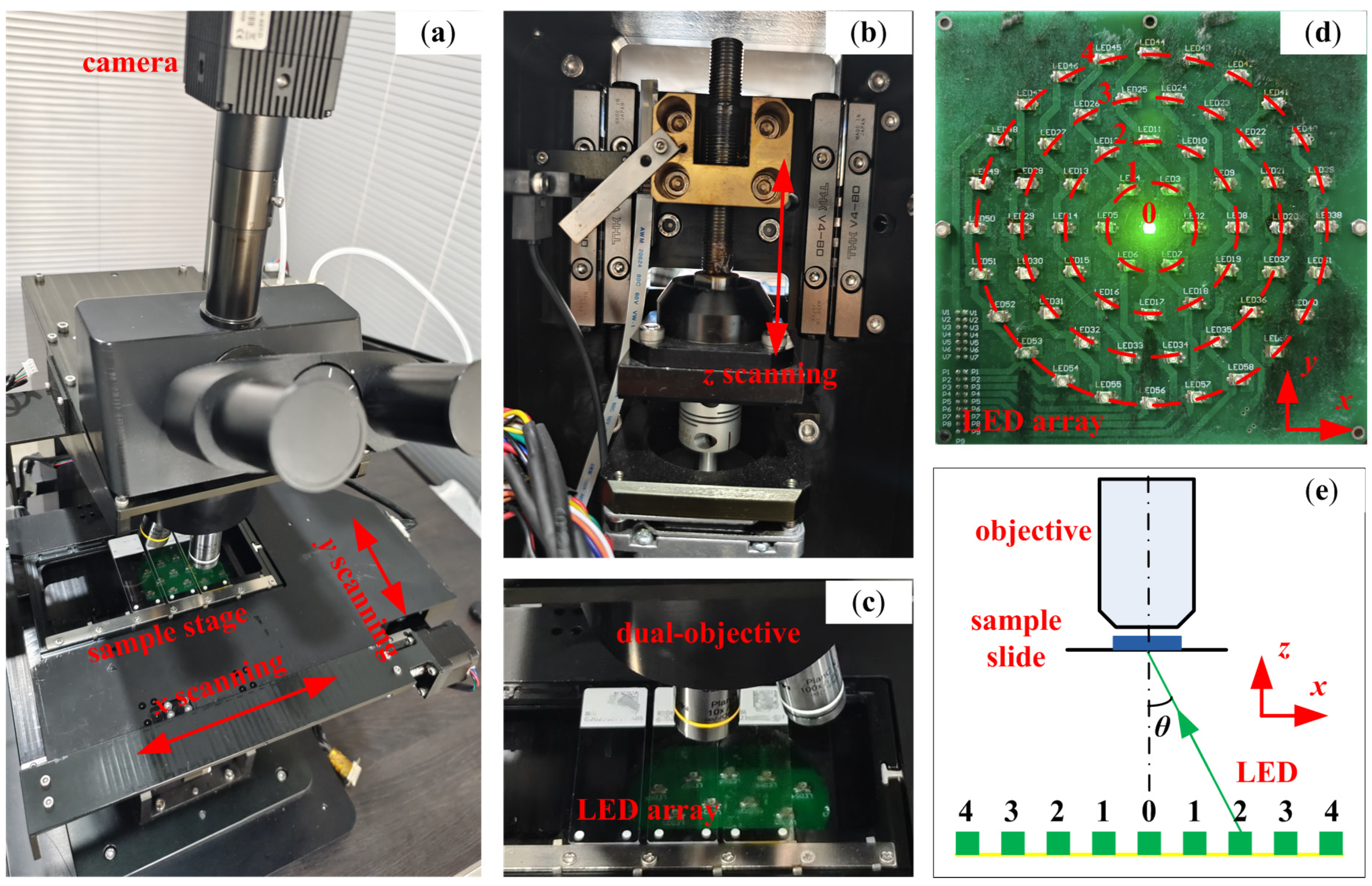
2.1. Hardware Platform

Figure 1a shows a bespoke automatic metaphase chromosome microscopy imaging platform detailed in this paper, comprising three integral components: the mechanical motion system, the imaging system, and the illumination system. The mechanical motion system incorporates an x-y motorized scanning stage designed for whole-slide scanning of chromosomes and precise positioning of metaphase chromosomes. This stage is driven by x and y stepper motors, facilitating precise ball-screw translation to enable scanning of the sample along both x and y axes. The scanning range extends to 210 × 120 mm, with the capacity to simultaneously scan up to six slides. The stage boasts a minimum step size of 0.04 μm, ensuring meticulous scanning resolution. The z-axis is equipped with a precision focusing mechanism, as shown in Figure 1b, which achieves high-resolution focusing through a fine lead screw manipulated by a stepper motor, featuring a minimum step size of 0.02 μm. A grating scale (Micro-E Optira series, with a resolution of 0.05 μm) is integrated to serve as a reference for precise positioning along the z-axis. The positional data gleaned from the grating scale are instrumental in calculating the defocus distance and orientation, thereby enhancing the autofocusing accuracy and efficiency of the system.

Within the imaging system, we employ a monochrome sCMOS camera (Dhyana 401D, Tucsen, 2048 × 2048 pixels, 6.5 μm pixel pitch) to acquire digital images with high clarity and speed. The imaging system is of the infinity-corrected optical variety, featuring a tube lens with a 180 mm focal length. It is complemented by an Olympus 10×, 0.25 numerical aperture (NA) objective (PLN10X) for chromosome large-field scanning and identification, as well as a 100×, 1.25 NA oil immersion objective (PLN100XO) for high-resolution imaging, as shown in Figure 1c. The dual-objective unit seamlessly uses an electric turret, allowing for an automated switch between low and high magnification objectives.

In the illumination system, our platform employs a programmable green LED array, serving as a substitute for conventional Kohler illumination and aperture. We have opted for green LEDs with a wavelength of 524 nm. The green spectrum is particularly effective in enhancing the contrast of chromosome samples stained with Giemsa, facilitating clearer imaging. The light source consists of 61 LEDs evenly distributed in a circular pattern, which is divided into a central LED and four rings of oblique illumination LEDs, providing uniform bright-field illumination for the imaging system, as shown in Figure 1d. The LED array’s luminosity is tunable, ensuring it aligns with the illumination demands for both low and high magnification objectives. The four rings of light sources have diameters of 30 mm, 60 mm, 90 mm, and 120 mm, respectively. The oblique illumination NA for each ring of LEDs is determined by the angle θ between the illumination light and the optical axis, as shown in Figure 1e, where NA = sin θ. The four symmetrical oblique illumination NAs that can be provided are 0.24, 0.45, 0.60, and 0.71. During metaphase chromosome imaging, the programmable LED array operates with flexibility, capable of providing independent oblique illumination for autofocusing or activating multiple or all LEDs for bright-field illumination.

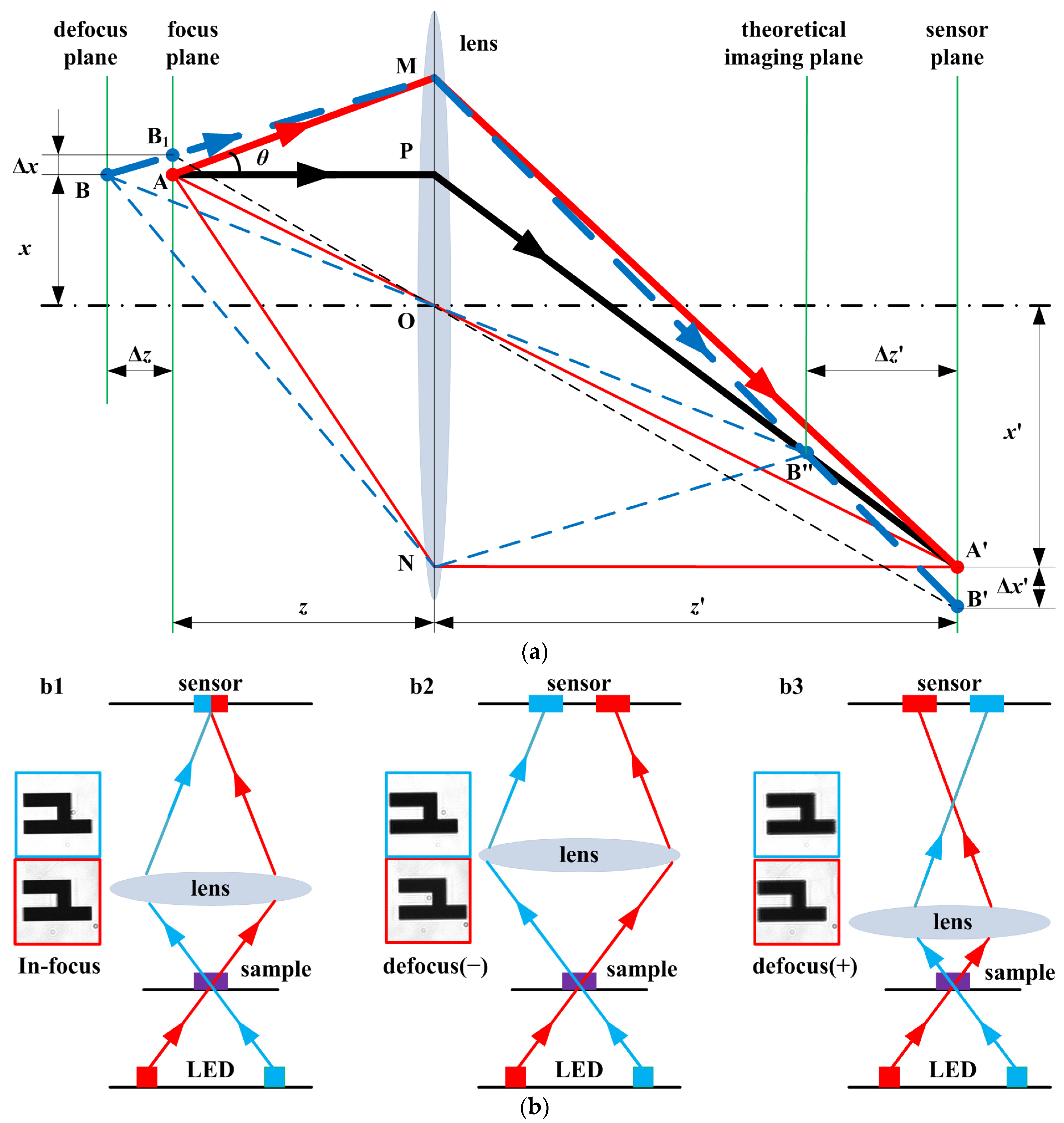
2.2. Rapid Autofocus Method Based on LED Oblique Illumination for Dual-Objective Unit

We build a model to illustrate that oblique illumination can cause defocused samples to experience pixel shifts on the camera sensor. As shown in Figure 2a, we represent the optical system with a single lens. The plane perpendicular to the optical axis where point A is located is the focus plane. The distance from the focal plane to the lens plane is z, and the distance from point A to the optical axis is x. The plane perpendicular to the optical axis where point B is located is the defocused plane, with a defocus distance of Δz. When the light is incident perpendicularly, the chief ray for imaging is AP, at which point A forms an image at point A′ on the camera sensor plane. The distance between the camera sensor plane and the lens plane is z′. When the light is incident at an angle θ, the chief ray for the image of point A is AM, and the image of point A on the sensor plane is still point A′. The chief ray for the imaging of point B is BM. The intersection of BM with the focus plane is point B1, and the distance between B1 and point A is denoted by Δx. Since Δz is far smaller than z, it can be considered that BM is parallel to AM, and the angle with the optical axis is also θ. At this moment, the theoretical image position of point B is denoted as B″, and the plane perpendicular to the optical axis on which B″ lies is called the theoretical image plane. However, the position of the sensor plane remains unchanged, and the actual center of the image of point B on the sensor plane is point B′. On the sensor plane, the horizontal shift of point B′ relative to point A′ is denoted by Δx′. From the geometric relationship in Figure 2a, the following equation can be derived:

$${\displaystyle \frac{\Delta x^{\prime }}{\Delta x}}={\displaystyle \frac{\left|{\mathrm{A}}^{\prime }\mathrm{O}\right|}{\left|\mathrm{AO}\right|}}={\displaystyle \frac{z^{\prime }}{z}},\mathsf{\Delta }x=\mathsf{\Delta }z\tan \theta ,$$

(1)

Equation (1) can be further organized as follows:

$$\mathsf{\Delta }{x}^{\prime }={\displaystyle \frac{z^{\prime }}{z}}\tan \theta \cdot \mathsf{\Delta }z,$$

(2)

where ${\displaystyle \frac{z^{\prime }}{z}}$ is a constant that depends only on the imaging system, while tanθ is related to the illumination angle. When the imaging system and illumination angle remain constant, the pixel offset captured by the sensor is linearly related to the defocus amount of the sample. In our method, we employ two LEDs for oblique illumination from different angles to achieve a greater pixel shift. Figure 2b shows a schematic diagram of two symmetrically oblique LEDs illuminating the sample from two opposing incident angles. When the sample is perfectly aligned at the focus position, the images obtained from the two LEDs almost overlap, as shown in Figure 2b1. However, when the sample is positioned at a negative defocus, there is a noticeable shift in pixels between the two images, as shown in Figure 2b2. Conversely, when the sample is at a positive defocus, the pixel shift is reversed, as shown in Figure 2b3. These pixel shifts are indicative of the defocus direction and distance. As the defocus distance of the sample increases, so does the pixel shift between the two images.

The magnitude of the pixel shift can be accurately quantified through image registration algorithms. Image cross-correlation calculation is a commonly used fast image registration algorithm. [21] The normalized cross-correlation coefficient between two images can be articulated using the following equation [28]:

$$\gamma \left(u,v\right)={\displaystyle \frac{{\displaystyle {\sum }_{x,y}\left[f\left(x,y\right)-{\overline{f}}_{u,v}\right]\left[t\left(x-u,y-u\right)-\overline{t}\right]}}{{\left\{{\displaystyle {\sum }_{x,y}{\left[f\left(x,y\right)-{\overline{f}}_{u,v}\right]}^2{\displaystyle {\sum }_{x,y}{\left[t\left(x-u,y-v\right)-\overline{t}\right]}^2}}\right\}}^{0.5}}},$$

(3)

where f(x, y) is the gray value of point (x, y) in the image, t(x, y) is the gray value of point (x, y) in the template, $\overline{t}$ is the mean of the template, ${\overline{f}}_{u,v}$ is the mean of f(x, y) in the region under the template. For example, we perform cross-correlation on two 200 × 200 pixels images as shown in Figure 3a and obtain the normalized cross-correlation curve as shown in Figure 3b. The pixel shift between two images is quantified by the discrepancy between the peak position of their cross-correlation function and the central position. To simplify the calculation, the symmetric illumination used for focusing is located on the x direction, the pixel shift in the y direction is typically negligible, and the analysis can focus solely on the x direction shift. The objective executes scans along the z-axis to capture images under illumination from two LEDs at distinct defocus settings, from which the pixel shift is deduced. By fitting a focus curve, the correlation between defocus distance and pixel shift is established, as the red scatter points and green line shown in Figure 3c. In the ensuing rapid autofocusing procedure, only two images illuminated obliquely by the LEDs are required. The defocus distance and direction are ascertained in real time by applying cross-correlation calculation to determine the pixel shifts and then substituting these values into the focus curve. A single adjustment of the objective position suffices to achieve autofocus, without scanning along the z-axis.

Our method relies on the computation of information captured by each pixel of the camera sensor. In practical applications, we have noticed that the focusable range of our method is limited. Beyond this range, the calculated pixel shift no longer exhibits a clear linear relationship with the defocus distance, as shown by the black scatter point in Figure 3c. The concept of energy on detector (EOD) introduced by Strojnik provides a compelling explanation for this phenomenon [29]. In optical systems, due to the diffraction, the image of a point source on the imaging plane forms a circular Airy disk [30]. Owing to the constraints of pixel dimensions, a single pixel cannot capture the entire energy of the imaged point source. For a rectangular pixel with an area of 4xy (pixel dimensions 2x by 2y), assuming the centroid of the point source image is at the pixel center, the energy enclosed within the pixel can be expressed by the following equation [29]:

$$EOD\left(d_x,d_y\right)={\displaystyle \frac{{\displaystyle {\int }_{-d_y}^{d_y}{\displaystyle {\int }_{-d_x}^{d_x}psf\left(x,y\right)dxdy}}}{{\displaystyle {\int }_{-\infty }^{\infty }{\displaystyle {\int }_{-\infty }^{\infty }psf\left(x,y\right)dxdy}}}},$$

(4)

where psf(x, y) is the point spread function of the optical system. The latest research indicates that when the specimen is severely defocused, the EOD of the central pixel noticeably decreases (from ~0.9 to ~0.3), with a greater amount of energy being distributed to the neighboring pixels [31]. The pixel with the highest energy cannot represent the true imaging position and possesses an unavoidable randomness. The coma aberration in the optical system can further reduce the EOD of the central pixel under oblique illumination. Influenced by these factors, the image captured on the sensor becomes very blurry, making it impossible to accurately calculate the pixel shift. Figure 4 displays chromosome sample images captured under single LED oblique illumination using 100× oil immersion objective. It is evident that metaphase chromosome images appear clear at the in-focus position, as shown in Figure 4a. When the defocus is minimal, the chromosome image retains its integrity and is clearly distinguishable from the background, as shown in Figure 4b. However, as the defocus distance increases, the chromosome image undergoes considerable distortion and becomes highly integrated with the background, as shown in Figure 4c.

The slope of the focus curve in Figure 3c is inherently linked to the NA of the illumination system for a given objective. An increased illumination NA correlates with a steeper curve slope, enhancing the focusing sensitivity. However, this heightened sensitivity comes with trade-offs: image distortion is exacerbated, background blending becomes more pronounced, and the precision of image registration diminishes, while the focusable range becomes narrowed. Consequently, the system’s focal range is contingent upon the DOF of the objective and the illumination NA. However, we cannot obtain this result through precise theoretical calculation. It requires the integration of objective and light source parameters, as well as necessary preliminary experiments, to explore. The DOF for an optical system can be theoretically determined to provide a benchmark value. For a microscopy imaging system equipped with a digital camera, the DOF is commonly approximated using the following equation [32]:

$${\mathsf{\Delta }}_{total}={\displaystyle \frac{2n}{\beta NA}}p+{\displaystyle \frac{n{\lambda }_0}{N{A}^2}},$$

(5)

where n is the refractive index in object space, β and NA are the magnification and numerical aperture of objective, λ₀ is the wavelength of the illumination, and p is the pixel size of the camera.

From the DOF calculation equation, the theoretical DOFs for the 10× objective and the 100× oil immersion objective utilized on the platform are determined to be 13.6 μm and 0.7 μm, respectively. Given the unique requirement for continuous focusing with dual-objective configuration in the metaphase chromosome imaging system, it is imperative to ensure that the focusing errors for both objectives remain beneath the DOF thresholds of their respective objectives to achieve clear imaging. Additionally, it is crucial to guarantee that the focusing error of the 10× objective falls within the focusable range of the 100× immersion oil immersion objective to accomplish the seamless focusing function of the dual-objective setup. Drawing on previous research findings and conducting preliminary experiments, the optimal NA values for the oblique illumination are selected for both types of objectives [20,21,22,23,24,25,26]. In our system, the 10× objective employs an oblique illumination NA of 0.24 (first ring), offering a focusable depth of approximately ±60 μm. Conversely, the 100× oil immersion objective utilizes an oblique illumination NA of 0.60 (third ring), providing a focusable range of approximately ±3 μm.

3. Experimental Results

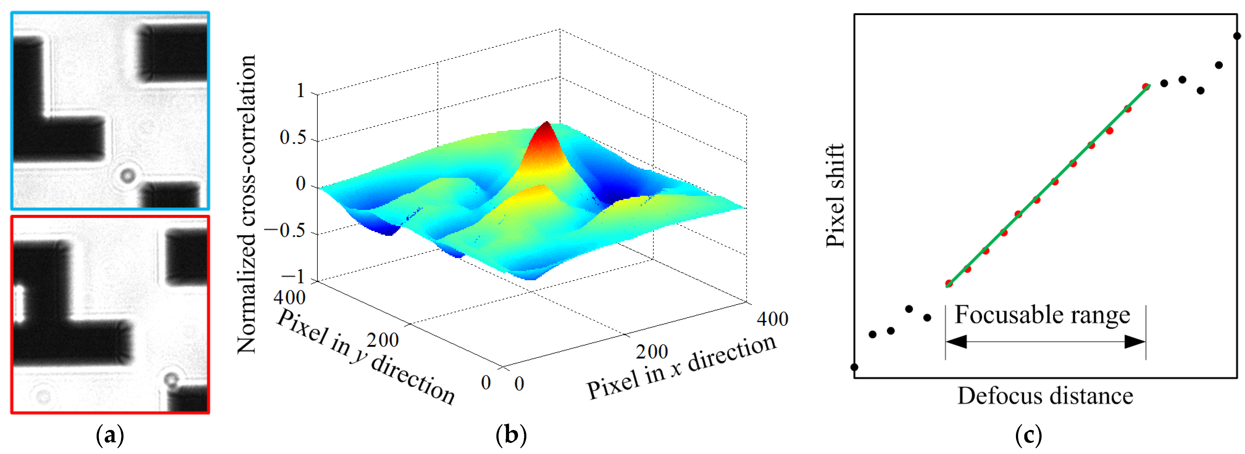
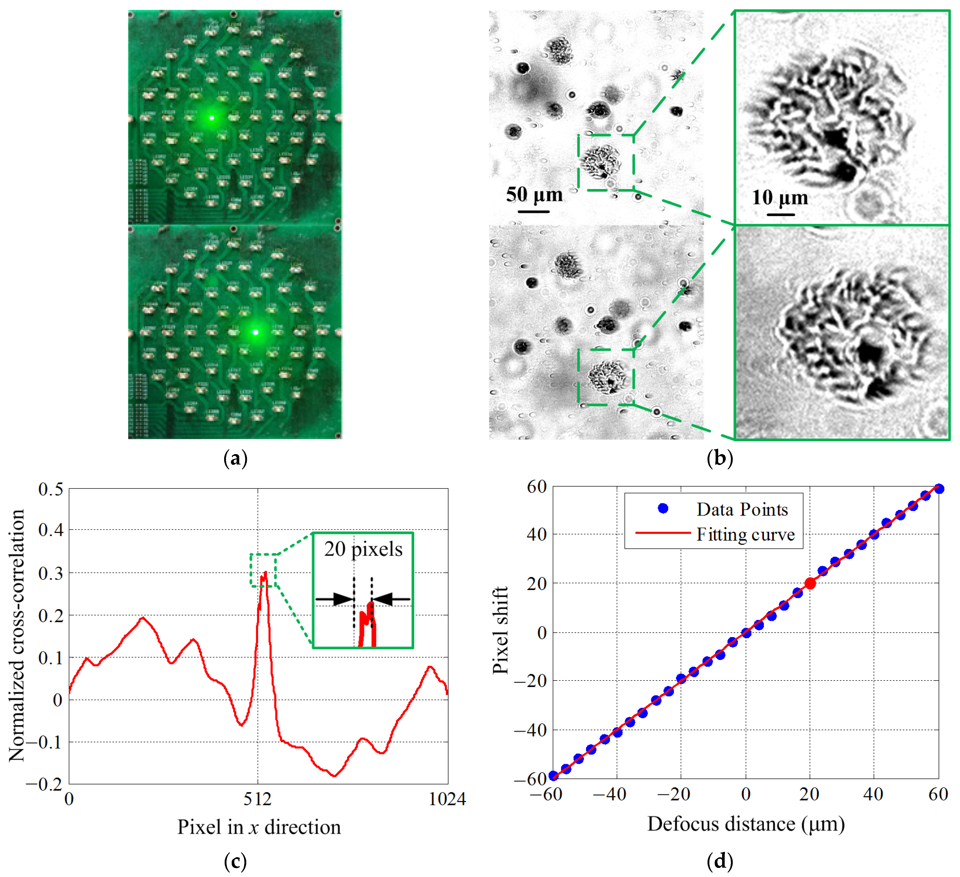
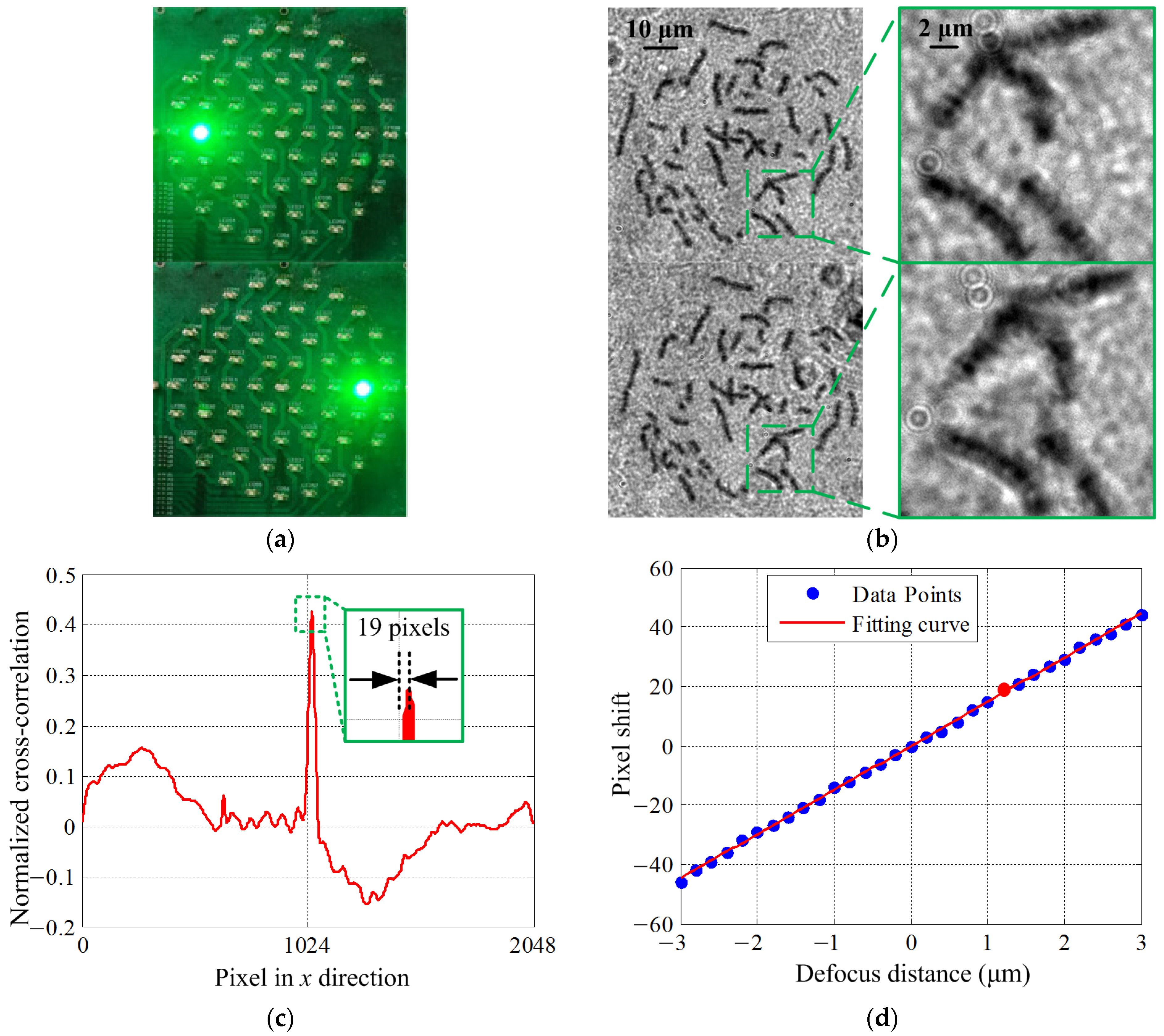
3.1. Dual-Objective Focus Curve Fitting

We initially proceed with the fitting of the focus curve for the 10× objective. As shown in Figure 5a, two symmetrical LEDs positioned in the x direction at the 0.24 NA setting are employed for oblique illumination at a reduced brightness to acquire images. Within the focusable range of ±60 μm, images are captured at intervals of 4 μm. A set of defocus images, each with a resolution of 512 × 512 pixels, is presented in Figure 5b. Cross-correlation calculation is executed, with the results for the x-direction as shown in Figure 5c. Based on the shift of the cross-correlation peak position from the central position, the pixel shift between the two images is determined to be 20 pixels. At this time, the corresponding defocus distance is 20 μm, and their relationship can be represented by the red point in Figure 5d. Leveraging the cross-correlation calculation outcomes from all captured positions, a relationship curve mapping the pixel shift to the z-direction grating ruler position coordinates is constructed. Subsequently, the focus curve for the 10× objective is derived and shown in Figure 5d.

Next, we apply the same methodology to determine the focus curve for the 100× oil immersion objective. As shown in Figure 6a, two symmetrical LEDs positioned in the x direction at the 0.60 NA setting are employed for oblique illumination at an elevated brightness to acquire images. Within the focusable range of ±3 μm, images are captured at intervals of 0.2 μm. To fully capture the metaphase chromosome image, a set of images with a resolution of 1024 × 1024 pixels, as shown in Figure 6b, are obtained for cross-correlation calculation, with the results of x-direction cross-correlation shown in Figure 6c. Based on the shift of the cross-correlation peak position from the central position, the pixel shift between the two images is determined to be 19 pixels. At this time, the corresponding defocus distance is 1.2 μm, and their relationship can be represented by the red point in Figure 6d. Leveraging the cross-correlation calculation outcomes from all captured positions, a relationship curve correlating the pixel shift with the z-direction grating ruler position coordinates is charted. Consequently, the focus curve for the 100× oil immersion objective is established and displayed in Figure 6d.

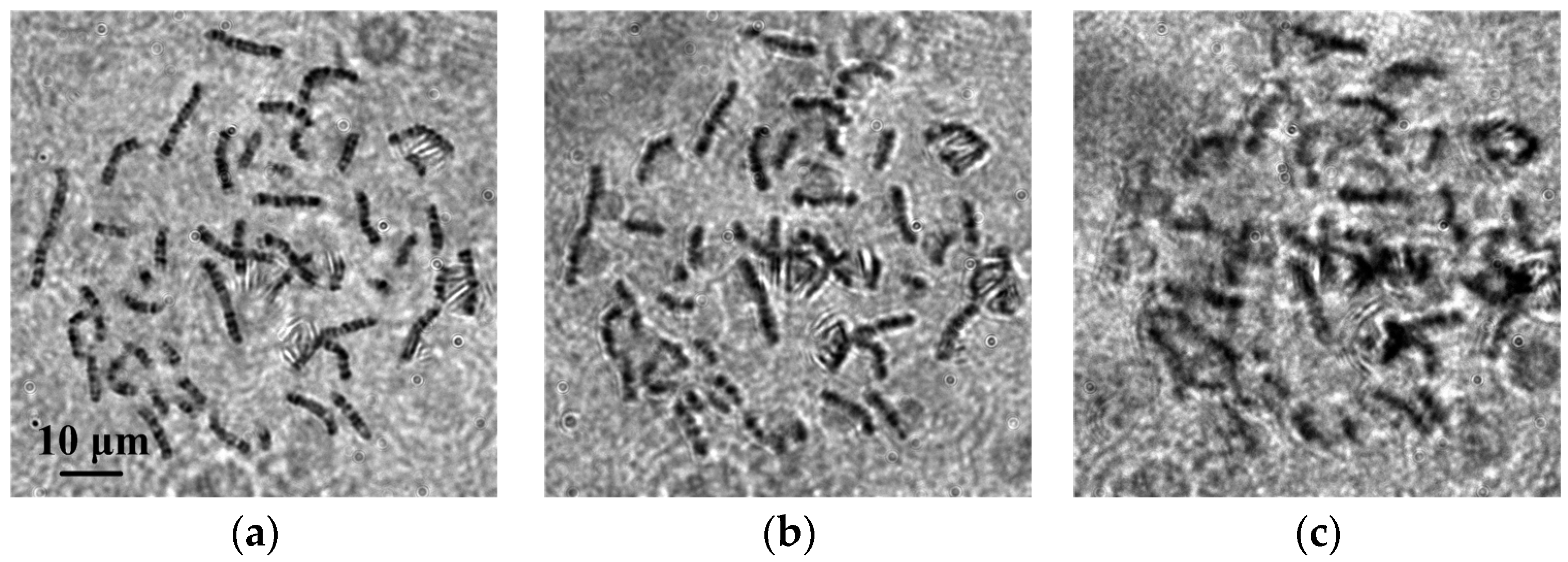
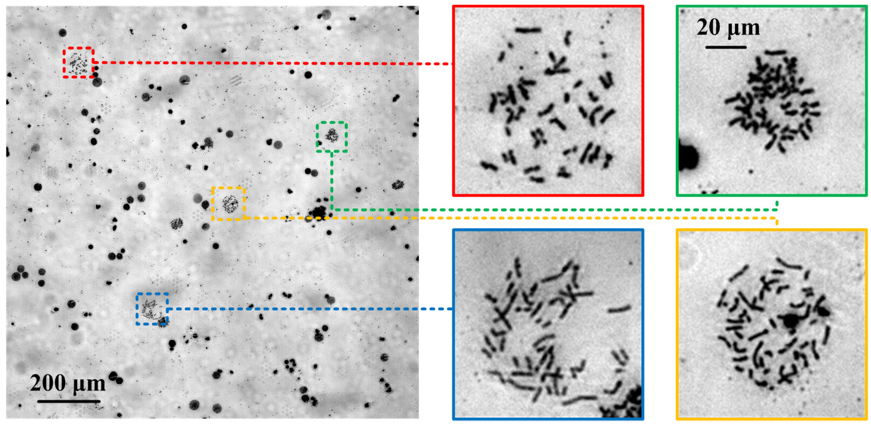
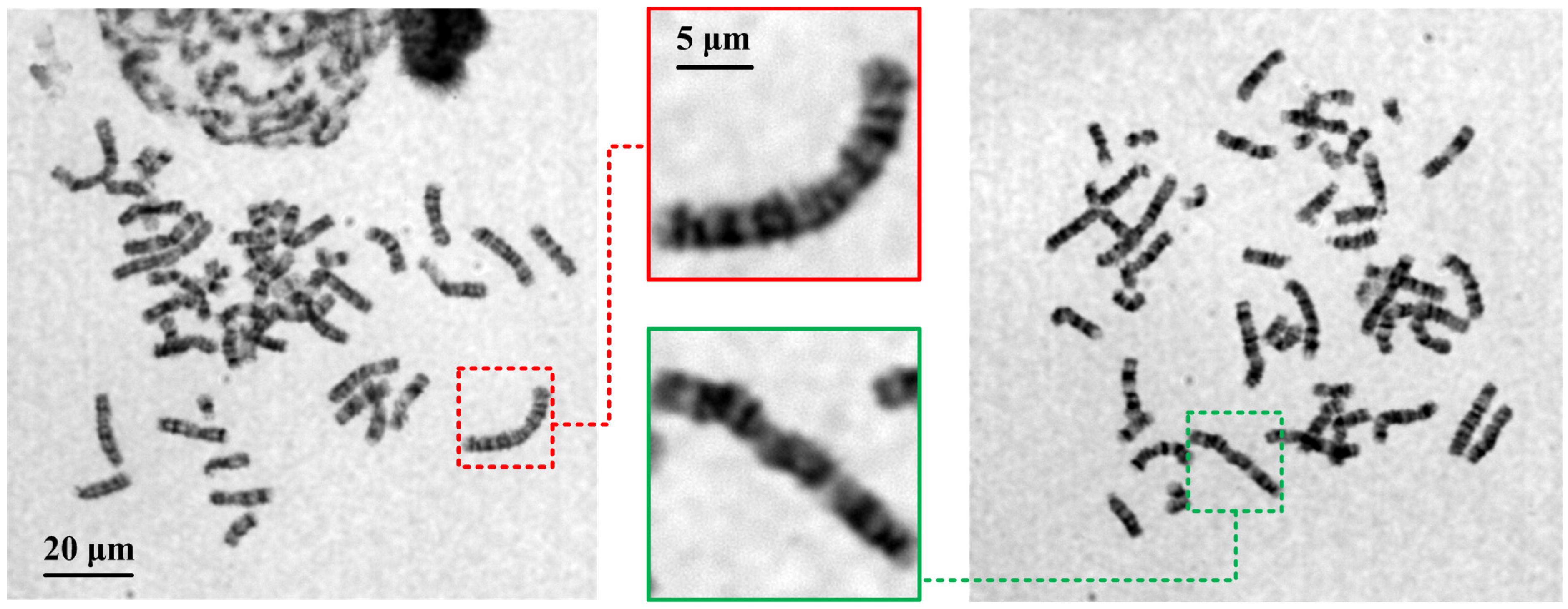
3.2. Chromosome Whole-Slide Autofocusing Experiments

We first conducted a rapid autofocus experiment using the 10× objective. The formal scanning procedure under the 10× objective primarily encompasses five steps: (1) Illuminate the FOV with a single LED on one side for oblique illumination to capture an image. (2) Illuminate the FOV with the symmetric LED and capture another image. (3) Extract the central 512 × 512 pixel section from the original image to compute the cross-correlation between the two images for the pixel shifts. These shifts are then applied to the focus curve to ascertain the defocus distance. (4) Activate the center and the first ring of a total of 7 LEDs for bright-field illumination, adjust the objective to the in-focus position along the z-axis, and capture the image to search for metaphase chromosomes; (5) Move the x-y stage to next FOV. Repeat steps (1) to (5) to complete the whole-slide scanning of the sample under the 10× objective.

In this work, metaphase chromosomes were identified by offline manual methods, and the x-y-z coordinates of these chromosomes were logged for high-resolution imaging with the 100× oil immersion objective. The bright-field original image of 2048 × 2048 pixels and the recognition result of the metaphase chromosomes are shown in Figure 7.

Subsequently, we conducted a rapid autofocusing experiment using the 100× oil immersion objective. The formal scanning protocol under the 100× oil immersion objective similarly comprises five key steps: (1) Illuminate the FOV with a single LED on one side for oblique illumination, and capture an image. (2) Illuminate the FOV with the symmetric LED and capture another image. (3) Extract the 1024 × 1024 pixel region from the original image which contains the entire chromosome to compute the cross-correlation between the two images for the pixel shifts. These shifts are then utilized in the focus curve to calculate the defocus distance. (4) Activate all 61 LEDs for bright-field illumination, and adjust the z-axis of the objective to the in-focus position to capture the high-resolution image. (5) Move the x-y stage to next FOV containing metaphase chromosomes. Repeat steps (1) to (5) to accomplish high-resolution imaging of all identified metaphase chromosomes under the 100× oil immersion objective, and archive the images for karyotype analysis. The bright-field original images, each 1024 × 1024 pixels in resolution, for two metaphase chromosomes after autofocusing are shown in Figure 8. Although we did not use Kohler illumination, the bright-field images still clearly show the banding information of the chromosomes.

3.3. Evaluation of Autofocusing Performance

To quantitatively assess the rapid autofocusing capabilities of the metaphase chromosome imaging system in this experiment, we primarily conducted experimental evaluations autofocusing on two critical aspects: focusing accuracy and focusing speed. We evaluated the continuous focusing performance on three different chromosome sample slides under dual-objective conditions. The standard value for the in-focus position is typically ascertained either manually by experts or through image processing algorithms. In this study, we employed the Brenner gradient method to determine the standard in-focus position for each imaging FOV. Originally introduced in 1976, the Brenner gradient method is an assessment technique that computes the square of the difference between its two contiguous pixels and then adds them together using the following equation [33]:

$$B={\displaystyle {\sum }_{x,y}{\left(i\left(x+1,y\right)-i\left(x-1,y\right)\right)}^2},$$

(6)

where i(x, y) is the intensity at pixel (x, y). The Brenner gradient is acutely sensitive to focus, monotonically decreasing and symmetric about the peak. It is widely used in autofocus algorithms for various biological samples. This method has also been applied to the autofocusing of metaphase chromosomes and has received better evaluations than others [13].

We initially assessed the focusing accuracy of the 10× objective across 288 FOVs within a 15 × 30 mm scanning area on each chromosome sample slide. The findings are graphically represented as a scatter plot shown in Figure 9. The focusing errors for the trio of samples are recorded at 1.19 ± 1.48 μm, 1.29 ± 1.55 μm, and 1.38 ± 1.64 μm, with an overall error of 1.29 ± 1.59 μm. The experimental data indicate that the mean focusing error significantly undercuts the DOF for the 10× objective, which extends to ±6.8 μm. Crucially, the focusing error for over 95% of the FOVs remains beneath the ±3 μm threshold, a range that falls within the focusable scope of the 100× oil immersion objective. This implies that the focal plane ascertained by the rapid autofocusing mechanism of the 10× objective is directly applicable for subsequent focusing computations with the 100× oil immersion objective. The FOVs that exhibit excessive focusing errors are predominantly attributed to sparse sample distribution or other contaminants that impede the computation of image cross-correlation.

During the search for well-dispersed metaphase chromosomes, we identified 158, 147, and 126 chromosomes on three separate slides. Subsequently, we evaluated the focusing error of the 100× oil immersion objective at these specific chromosome locations, with the results shown as a scatter plot in Figure 10. The focusing errors for the three samples are reported as 0.11 ± 0.14 μm, 0.12 ± 0.15 μm, and 0.13 ± 0.15 μm, averaging to an overall error of 0.12 ± 0.15 μm. The experimental outcomes confirm that the mean focusing error is well below the DOF for the 100× oil immersion objective, specified as ±0.35 μm, with 97% of the outcomes falling within this range. This evidence substantiates the efficacy of our dual-objective rapid autofocus method for whole-slide imaging of metaphase chromosomes, underscoring its suitability for high-precision imaging applications.

Next, we assessed the focusing speed of our dual-objective system using a desktop computer (Intel i7-3930, 3.2 GHz, 32 GB RAM). The image acquisition process for the 10× objective encompasses the five steps outlined in Section 3.2. The mean duration for each step is as follows: step 1 takes~ 0.02 s; step 2 takes ~0.02 s; step 3 takes ~0.03 s; step 4 takes ~0.07 s; step 5 takes ~0.20 s. Consequently, the time for a complete cycle is ~0.34 s, as shown in Figure 11a. The aggregate time needed to scan a 15 × 30 mm area across 288 FOVs on a single slide is approximately 98 s. The image acquisition process for the 100× oil immersion objective is similar to the 10× scanning procedure, with a key distinction: it foregoes the need for individual FOV scanning, focusing solely on areas where metaphase chromosomes are detected. The time for a single cycle is ~0.44 s (step 1 takes~ 0.03 s; step 2 takes ~0.03 s; step 3 takes ~0.06 s; step 4 takes ~0.08 s; step 5 takes ~0.24 s), as shown in Figure 11b. The cumulative time required for image acquisition with the 100× oil immersion objective, capturing images of a sample with 50 metaphase chromosomes, is approximately 22 s. Based on these experimental findings, our dual-objective rapid autofocus method demands a total time of roughly 120 s, or 2 min, for capturing a slide with 50 metaphase chromosomes. This is a stark contrast to traditional methods, which entail capturing 20 z-stacks per FOV, consuming approximately 10 min. Our method thus offers a marked advantage in terms of speed for whole-slide scanning in chromosome imaging.

4. Conclusions and Discussion

In summary, we report a rapid autofocus method based on LED oblique illumination and image cross-correlation calculation, applied to the metaphase chromosome whole-slide microscopy imaging system. Our method involves capturing two images by activating two green LEDs in sequence for oblique illumination. The defocus distance and direction are ascertained by employing a cross-correlation algorithm to measure the pixel shift between the two images. Subsequently, the z-axis position of the objective is precisely adjusted to achieve rapid autofocusing. Once the focus is achieved, multiple LEDs can be illuminated at once to provide bright-field lighting for image acquisition.

The chromosome imaging process differs from other imaging tasks mainly in two aspects. Firstly, it necessitates switching between two objectives to perform whole-slide scanning and high-resolution imaging. Secondly, achieving high-resolution chromosome banding requires a high NA oil immersion lens, characterized by a shallow DOF and a limited focus range. To address these challenges, we ensured not only that both objectives could independently achieve autofocusing, but also that the focusing result of the 10× objective can be continued for the final focusing of the 100× oil immersion objective. We optimized the illumination NA for continuous autofocusing by leveraging previous research and preliminary experiments, balancing between the focusable range and sensitivity. Our experimental results demonstrate that our autofocus method significantly outperforms traditional methods in terms of scanning speed with an excellent focusing accuracy. For the 10× objective, the average focusing error is substantially smaller than the system’s DOF, with over 95% of FOVs exhibiting a focusing error within ±3 μm, well within the 100× oil immersion objective’s focusable range. For the 100× oil immersion objective, more than 97% of the focus results are within the DOF, facilitating the acquisition of clear metaphase chromosome images.

In this study, our microscopy imaging was confined to metaphase chromosomes from blood samples, which is representative but not comprehensive. Future studies should encompass a broader range of samples, such as amniotic fluid, bone marrow, and products of conception, to enhance the generalizability of our findings. In addition, our rapid autofocus method also has the potential to be applied in the imaging of other samples. Moreover, leveraging the adaptability of programmable LED array, we intend to explore the integration of Fourier Ptychography Microscopy into chromosome imaging systems in future endeavors.

References

1. Natarajan, A.T. Chromosome aberrations: Past, present and future. Mutat. Res. 2002, 504, 3–16. [Google Scholar] [CrossRef] [PubMed]
2. Levy, B.; Wapner, R. Prenatal diagnosis by chromosomal microarray analysis. Fertil. Steril. 2018, 109, 201–212. [Google Scholar] [CrossRef] [PubMed]
3. Theisen, A.; Shaffer, L.G. Disorders caused by chromosome abnormalities. Appl. Clin. Genet. 2010, 3, 159–174. [Google Scholar] [PubMed]
4. Madian, N.; Jayanthi, K.B. Analysis of human chromosome classification using centromere position. Measurement 2014, 47, 287–295. [Google Scholar] [CrossRef]
5. Arora, T.; Dhir, R. A review of metaphase chromosome image selection techniques for automatic karyotype generation. Med. Biol. Eng. Comput. 2016, 54, 1147–1157. [Google Scholar] [CrossRef]
6. Grisan, E.; Poletti, E.; Ruggeri, A. Automatic segmentation and disentangling of chromosomes in Q-band prometaphase images. IEEE Trans. Inf. Technol. Biomed. 2009, 13, 575–581. [Google Scholar] [CrossRef]
7. Furukawa, A. The implementation of artificial intelligence to the low-cost metaphase finder. Radiat. Prot. Dosim. 2023, 199, 1460–1464. [Google Scholar] [CrossRef]
8. Wang, X.; Li, S.; Liu, H.; Wood, M.; Chen, W.R.; Zheng, B. Automated identification of analyzable metaphase chromosomes shown on microscopy digital images. J. Biomed. Inf. 2008, 41, 264–271. [Google Scholar] [CrossRef]
9. Bian, Z.; Guo, C.; Jiang, S.; Zhu, J.; Wang, R.; Song, P.; Zhang, Z.; Hoshino, K.; Zheng, G. Autofocusing technologies for whole slide imaging and automated microscopy. J. Biophotonics 2020, 13, e202000227. [Google Scholar] [CrossRef]
10. Hu, J.; Zhong, B.; Jin, Z.; Wang, Z.; Sun, L. Adaptive predictive scanning method based on a high-precision automatic microscopy system. Appl. Opt. 2019, 58, 7305–7310. [Google Scholar] [CrossRef]
11. Liu, C.-S.; Song, R.-C.; Fu, S.-J. Design of a laser-based autofocusing microscope for a sample with a transparent boundary layer. Appl. Phys. B 2019, 125, 199. [Google Scholar] [CrossRef]
12. Song, J.; Liu, M. A new methodology in constructing no-reference focus quality assessment metrics. Pattern Recognit. 2023, 142, 109688. [Google Scholar] [CrossRef]
13. Qiu, Y.; Chen, X.; Li, Y.; Chen, W.R.; Zheng, B.; Li, S.; Liu, H. Evaluations of auto-focusing methods under a microscopy imaging modality for metaphase chromosome image analysis. Anal. Cell. Pathol. 2013, 36, 37–44. [Google Scholar] [CrossRef]
14. Yilmaz, H.; Turan, M.K. FahamecV1: A Low Cost Automated Metaphase Detection System. Eng. Technol. Appl. Sci. Res. 2017, 7, 2160–2166. [Google Scholar] [CrossRef]
15. Furukawa, A.; Minamihisamatsu, M.; Hayata, I. Low-cost metaphase finder system. Health Phys. 2010, 98, 269–275. [Google Scholar] [CrossRef]
16. Furukawa, A. The project of another low-cost metaphase finder. Radiat. Prot. Dosim. 2016, 172, 238–243. [Google Scholar] [CrossRef]
17. Montalto, M.C.; McKay, R.R.; Filkins, R.J. Autofocus methods of whole slide imaging systems and the introduction of a second-generation independent dual sensor scanning method. J. Pathol. Inform. 2011, 2, 44. [Google Scholar] [CrossRef]
18. Guo, K.; Liao, J.; Bian, Z.; Heng, X.; Zheng, G. InstantScope: A low-cost whole slide imaging system with instant focal plane detection. Biomed. Opt. Express 2015, 6, 3210–3216. [Google Scholar] [CrossRef]
19. Li, C.; Liu, K.; Guo, X.; Xiao, Y.; Zhang, Y.; Huang, Z.L. Robust autofocus method based on patterned active illumination and image cross-correlation analysis. Biomed. Opt. Express 2024, 15, 2697–2707. [Google Scholar] [CrossRef]
20. Liao, J.; Bian, L.; Bian, Z.; Zhang, Z.; Patel, C.; Hoshino, K.; Eldar, Y.C.; Zheng, G. Single-frame rapid autofocusing for brightfield and fluorescence whole slide imaging. Biomed. Opt. Express 2016, 7, 4763–4768. [Google Scholar] [CrossRef]
21. Liao, J.; Jiang, Y.; Bian, Z.; Mahrou, B.; Nambiar, A.; Magsam, A.W.; Guo, K.; Wang, S.; Cho, Y.K.; Zheng, G. Rapid focus map surveying for whole slide imaging with continuous sample motion. Opt. Lett. 2017, 42, 3379–3382. [Google Scholar] [CrossRef] [PubMed]
22. Liao, J.; Wang, Z.; Zhang, Z.; Bian, Z.; Guo, K.; Nambiar, A.; Jiang, Y.; Jiang, S.; Zhong, J.; Choma, M.; et al. Dual light-emitting diode-based multichannel microscopy for whole-slide multiplane, multispectral and phase imaging. J. Biophoton. 2018, 11, e201700075. [Google Scholar] [CrossRef] [PubMed]
23. Jiang, S.; Bian, Z.; Huang, X.; Song, P.; Zhang, H.; Zhang, Y.; Zheng, G. Rapid and robust whole slide imaging based on LED-array illumination and color-multiplexed single-shot autofocusing. Quant. Imaging Med. Surg. 2019, 9, 82331–82831. [Google Scholar] [CrossRef]
24. Guo, C.; Bian, Z.; Jiang, S.; Murphy, M.; Zhu, J.; Wang, R.; Song, P.; Shao, X.; Zhang, Y.; Zheng, G. OpenWSI: A low-cost, high-throughput whole slide imaging system via single-frame autofocusing and open-source hardware. Opt. Lett. 2020, 45, 260–263. [Google Scholar] [CrossRef]
25. Guo, C.; Bian, Z.; Alhudaithy, S.; Jiang, S.; Tomizawa, Y.; Song, P.; Wang, T.; Shao, X. Brightfield, fluorescence, and phase-contrast whole slide imaging via dual-LED autofocusing. Biomed. Opt. Express 2021, 12, 4651–4660. [Google Scholar] [CrossRef]
26. Xin, K.; Jiang, S.; Chen, X.; He, Y.; Zhang, J.; Wang, H.; Liu, H.; Peng, Q.; Zhang, Y.; Ji, X. Low-cost whole slide imaging system with single-shot autofocusing based on color-multiplexed illumination and deep learning. Biomed. Opt. Express 2021, 12, 5644–5657. [Google Scholar] [CrossRef]
27. Zheng, G.; Horstmeyer, R.; Yang, C. Wide-field, high-resolution Fourier ptychographic microscopy. Nat. Photonics 2013, 7, 739. [Google Scholar] [CrossRef]
28. Lewis, J.P. Fast normalized cross-correlation. Vis. Interface 1995, 10, 120–123. [Google Scholar]
29. Strojnik, M.; Bravo-Medina, B.; Martin, R.; Wang, Y. Ensquared energy and optical centroid efficiency in optical sensors: Part 1, Theory. Photonics 2023, 10, 254. [Google Scholar] [CrossRef]
30. Born, M.; Wolf, E. Principles of Optics, 7th ed.; Cambridge University Press: Cambridge, UK, 1999. [Google Scholar]
31. Strojnik, M.; Martin, R.; Wang, Y. Ensquared energy and optical centroid efficiency in optical sensors: Part 2, Primary Aberrations. Photonics 2024, 11, 855. [Google Scholar] [CrossRef]
32. Qiu, Y.; Chen, X.; Li, Y.; Zheng, B.; Li, S.; Chen, W.R.; Liu, H. Impact of the optical depth of field on cytogenetic image quality. J. Biomed. Opt. 2012, 17, 096017. [Google Scholar] [CrossRef] [PubMed]
33. Brenner, J.F.; Dew, B.S.; Horton, J.B.; King, T.; Neurath, P.W.; Selles, W.D. An automated microscope for cytologic research a preliminary evaluation. J. Histochem. Cytochem. 1976, 24, 100–111. [Google Scholar] [CrossRef] [PubMed]
Figure 1. Metaphase chromosome microscopy imaging platform. (a) Structure of the microscopy imaging system. (b) Z-axis autofocusing unit. (c) Dual-objective unit. (d) Programmable LED array illumination unit. (e) Schematic diagram of LED oblique illumination.
Photonics 11 01091 g001
Figure 2. (a) Oblique illumination defocus sample model. (b) Schematic diagram of two symmetrically oblique LEDs in our autofocus method, (b1b3) are in-focus images, negative defocus images, positive defocus images under oblique illumination, respectively.
Photonics 11 01091 g002
Figure 3. An example for cross-correlation calculating and focus curve fitting. (a) Two example images. (b) Normalized cross-correlation curve of the two images. (c) Fitting curve of the relationship between pixel shift and defocus distance, the red scatter points are in focusable range, and the black scatter points are not.
Photonics 11 01091 g003
Figure 4. Chromosome sample images under single LED oblique illumination using 100× oil immersion objective. (a) Images at the in-focus position. (b) Images at a position with a small defocus distance. (c) Images at a position with a large defocus distance.
Photonics 11 01091 g004
Figure 5. Fitting of the focus curve for chromosome samples under 10× objective. (a) Illumination LEDs used. (b) Images obtained by alternating illumination with dual-LED. (c) Normalized cross-correlation curve of the two images in the x direction. (d) Fitting curve of the relationship between pixel shift and defocus distance, and the red point is the data in (c).
Photonics 11 01091 g005
Figure 6. Fitting of the focus curve for chromosome samples under 100× oil immersion objective. (a) Illumination LEDs used. (b) Images obtained by alternating illumination with dual-LED. (c) Normalized cross-correlation curve of the two images in the x direction. (d) Fitting curve of the relationship between pixel shift and defocus distance, and the red point is the data in (c).
Photonics 11 01091 g006
Figure 7. Bright-field image and metaphase chromosome recognition results after autofocusing with 10× objective.
Photonics 11 01091 g007
Figure 8. Bright-field images after autofocusing with 100× oil immersion objective.
Photonics 11 01091 g008
Figure 9. Focusing errors obtained by whole-slide scanning with 10× objective.
Photonics 11 01091 g009
Figure 10. Focusing errors in imaging chromosomes with 100× oil immersion objective.
Photonics 11 01091 g010
Figure 11. (a) Time for a single autofocusing cycle under 10× objective. (b) Time for a single autofocusing cycle under 100× oil immersion objective.
Photonics 11 01091 g011
Disclaimer/Publisher’s Note: The statements, opinions and data contained in all publications are solely those of the individual author(s) and contributor(s) and not of MDPI and/or the editor(s). MDPI and/or the editor(s) disclaim responsibility for any injury to people or property resulting from any ideas, methods, instructions or products referred to in the content.