Co-Phase Error Detection for Segmented Mirrors Based on Far-Field Information and Transfer Learning

Abstract

The resolution of a telescope is closely related to its aperture size; however, the aperture of a single primary mirror telescope cannot be indefinitely enlarged due to design and manufacturing constraints. Segmented mirror technology can achieve the same resolution as a single primary mirror of equivalent aperture, provided that the segments are co-phased correctly. This paper proposes a method for high-precision detection of piston errors in segmented mirror telescope systems, based on far-field information and transfer learning. By training a ResNet-18 network model, this method can predict piston errors with high precision within 10 ms of a single-frame far-field diffraction image. Simulation results demonstrate that the method is robust to tip-tilt errors, wavefront aberrations, and noise. This approach is simple, fast, highly accurate in detection, and resistant to noise, providing a new solution for piston error detection in segmented mirror systems.

1. Introduction

With the advancement of technology and the growing demand for space exploration, there are increasingly higher requirements for telescope design. According to the Rayleigh criterion, a telescope’s resolution is limited by the aperture size of its primary mirror; a larger primary mirror aperture translates to higher resolution and greater light-gathering capability. However, due to constraints in design, manufacturing, and processing costs, constructing a single-aperture primary mirror telescope with a diameter greater than 8 m is extremely challenging [1]. Synthetic aperture technology involves stitching together two or more segments to achieve a resolution and light-gathering capability equivalent to a single-aperture primary mirror. The European Southern Observatory (ESO) is constructing the Extremely Large Telescope (ELT) [2], whose primary mirror consists of 798 hexagonal segments; the Thirty Meter Telescope (TMT) features a segmented primary mirror composed of 492 hexagonal segments [3]; the Giant Magellan Telescope (GMT) is made up of seven 8.4 m primary mirrors [4]; and the James Webb Space Telescope (JWST), currently in orbit, has an 18-segment hexagonal primary mirror [5,6,7]. However, for these segmented mirrors to achieve the same resolution and light-gathering power as an equivalent single-aperture primary mirror, they must be optically co-phased. Piston error refers to the axial optical path difference of each segment relative to the same wavefront and must be constrained within a range of 0.05λ.

Since the introduction of synthetic aperture technology, numerous effective methods for detecting piston errors have been proposed by researchers worldwide, which can be broadly classified into two categories: pupil plane detection and focal plane detection. Pupil plane detection involves analyzing images of the pupil plane’s light intensity captured by sensors. Techniques in this category include the Shack–Hartmann broadband and narrowband phasing methods [8], curvature sensing [9], interferometry-based methods [10], pyramid wavefront sensing [11], dispersed fringe sensing [12,13,14], and Zernike phase contrast methods [15]. These methods are characterized by their high real-time performance, enabling rapid measurement of piston errors in segmented mirrors, but they increase the complexity of the optical system. Focal plane detection methods, on the other hand, utilize wavefront-free sensing techniques to capture light intensity information at or near the focal plane and calculate piston errors using specific algorithms. While this approach simplifies the optical system structure to some extent, it suffers from a narrow detection range, prolonged iterative processes, and poor convergence stability. Examples of such methods include phase retrieval [16], phase diversity [17], and modified particle swarm optimization algorithms [18].

In recent years, the rapid development of artificial intelligence has led to the interdisciplinary integration of deep learning and optics, offering new solutions for piston error detection. As early as 1990, Angel et al. in the United States first proposed a neural network-based approach for piston error detection across multiple telescopes [19]. In 2018, Guerra-Ramos et al. in Spain utilized a convolutional neural network (CNN) to detect piston errors in a 36-segment mirror system, overcoming the 2π phase range limitation using a four-wavelength system, achieving an accuracy of ±0.0087λ [20]. In 2019, Li Dequan and colleagues from the Changchun Institute of Optics, Fine Mechanics and Physics, Chinese Academy of Sciences developed a dataset using an M-sharpness function for target-independent piston error detection [21]. Concurrently, Ma Xiafei and her team from the Institute of Optics and Electronics, Chinese Academy of Sciences employed a deep convolutional neural network (DCNN) to model the relationship between the point spread function of a system and piston errors, validating the method’s feasibility through simulations and experiments [22]. In 2021, Wang et al. from the Xi’an Institute of Optics and Precision Mechanics of Chinese Academy of Sciences combined cumulative dispersed fringe pattern (LSR-DSF) with a deep CNN to achieve integrated coarse-to-fine piston error detection in segmented mirrors, maintaining the root mean square error within 10.2 nm over a range of ±139λ [23]. Neural networks offer high accuracy for piston error detection from single-frame images, but they require significant time for network training in the initial stages.

In this study, a pre-trained ResNet-18 network model was transferred to an optical system to learn the mapping relationship between far-field images and piston errors. The trained network can accurately predict the piston error between two segmented mirrors within 10 milliseconds, significantly improving the detection speed compared to traditional methods. Simulation verified the high accuracy and robustness of this approach and demonstrated its applicability in complex optical systems. Compared to previous detection methods that rely on complex system architectures and extensive data processing, the ResNet-18-based detection strategy proposed in this study greatly simplifies the error detection process, reduces system complexity, and provides a novel and efficient solution for future co-phasing error detection in segmented mirror systems.

2. Basic Principle

2.1. Mathematical Model

The core principle of convolutional neural networks (CNNs) in regression prediction tasks lies in their automated process of feature extraction, mapping, and optimization, which transforms key information from input diffraction images into continuous output variables. Specifically, CNNs first extract spatial features from images through a series of convolutional and pooling layers, encoding information closely related to the prediction target. These high-level features are then mapped to the output space via fully connected layers to generate the corresponding predicted values. After training, CNNs can directly predict the corresponding continuous variables from new input diffraction images using the learned features. The prediction accuracy is closely related to the sensitivity of the diffraction images to piston errors; the higher the sensitivity of the images to piston errors, the higher the prediction accuracy of the network. This study uses a two-segment mirror system as an example to construct the corresponding diffraction image and its labeled dataset, providing foundational data for training and testing deep learning models.

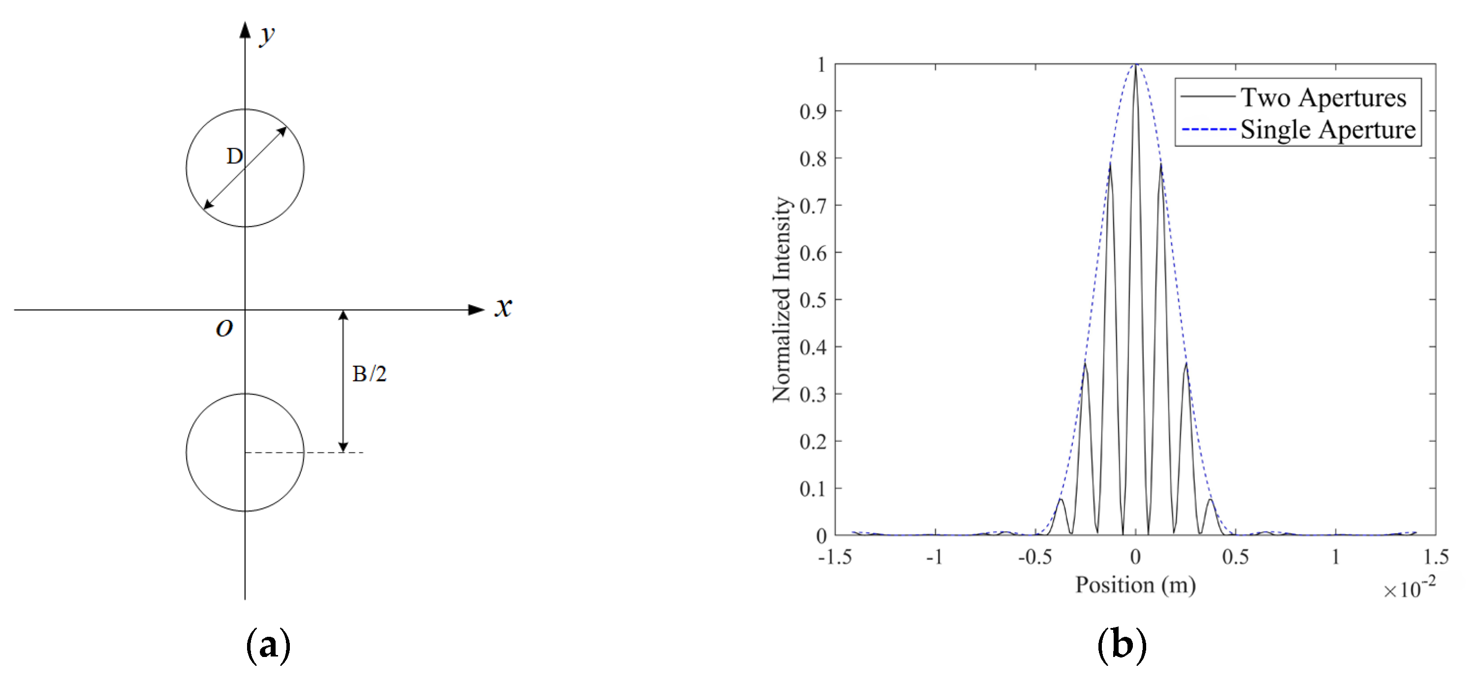
As shown in Figure 1, based on the principle of Fraunhofer diffraction through a circular aperture, a mask is placed at the exit pupil plane of two segmented mirrors. Parallel monochromatic light, after reflecting off the segmented mirrors, passes through the circular aperture and is coherently imaged onto the detector surface of a camera through a focusing lens. In this configuration, there is a strict one-to-one correspondence between the piston error of the two segmented mirrors and the diffraction intensity pattern on the camera’s detector surface. This arrangement ensures that changes in the diffraction image directly reflect the piston error of the segmented mirrors, providing a clear and explicit physical basis for error detection.

Assuming the diameter of the circular aperture is D and the coordinates of the center are $(0,{\displaystyle \frac{B}{2}})$ and $(0,-{\displaystyle \frac{B}{2}})$, the pupil function of the aperture in the pupil plane is given by

$$P\left(x,y\right)=circ(0,{\displaystyle \frac{B}{2}},D)+circ(0,-{\displaystyle \frac{B}{2}},D)$$

(1)

The phases of the circular apertures are denoted as ${\phi }_1$ and ${\phi }_2$, respectively, and the generalized pupil function at the exit pupil plane is given by

$$\mathcal{P}\left(x,y\right)=circ(0,{\displaystyle \frac{B}{2}},D)\cdot \mathrm{e}\mathrm{x}\mathrm{p} (i{\phi }_1)+circ(0,-{\displaystyle \frac{B}{2}},D)\cdot \mathrm{e}\mathrm{x}\mathrm{p} (i{\phi }_2)$$

(2)

The phase difference between the two circular apertures is denoted as $∆\phi$:

$$∆\phi ={\phi }_2-{\phi }_1={\displaystyle \frac{2\pi }{\lambda }}\cdot OPD$$

(3)

where λ represents the wavelength of the incident light wave, and OPD denotes the axial optical path difference between the two segmented mirrors, which corresponds to the piston error in this context.

According to the imaging principles of the optical system, the intensity point spread function (PSF) of the system is given by

$$PSF(u,v)={\displaystyle \frac{1}{{\lambda }^2{f}^2}}{\left|\mathcal{F}\left\{\mathcal{P}\right(x,y\left)\right\}\right|}^2$$

(4)

where f represents the focal length of the lens, and $\mathcal{F}\{\cdot \}$ denotes the Fourier transform operator.

The light intensity I on the detector surface of the camera can be expressed as

$$I(u,v)=o(u,v)⨂PSF(u,v)+n(u,v)$$

(5)

where $o(u,v)$ represents the ideal distribution of the point source, which is 1 in this case, $⨂$ represents the convolution operation, and $n(u,v)$ denotes the noise introduced by the camera.

From Equation (4), it can be seen that double-aperture diffraction results from the combined effects of single-aperture diffraction and interference. The normalized PSF of a single aperture and two apertures is shown in Figure 2. The single-aperture diffraction factor is related to the properties of the aperture itself, while the double-aperture interference term arises from the periodic arrangement of the apertures and is independent of the properties of the individual apertures.

2.2. Dataset Generation

To validate the feasibility of the neural network-based method for co-phasing piston error detection, a dataset needs to be constructed to establish the mapping relationship between diffraction images and piston errors. During the simulation phase, the optical imaging system is modeled in MATLAB based on the principles of Fourier optics, introducing co-phasing errors to generate a series of intensity diffraction images. The parameters were chosen based on the configuration of the JWST system, the diameter of the circular aperture, D = 0.15 m, the distance between the two circular apertures, B = 1.4 m, the focal length of the lens, f = 20 m, and the incident light wavelength, λ = 632.8 nm. 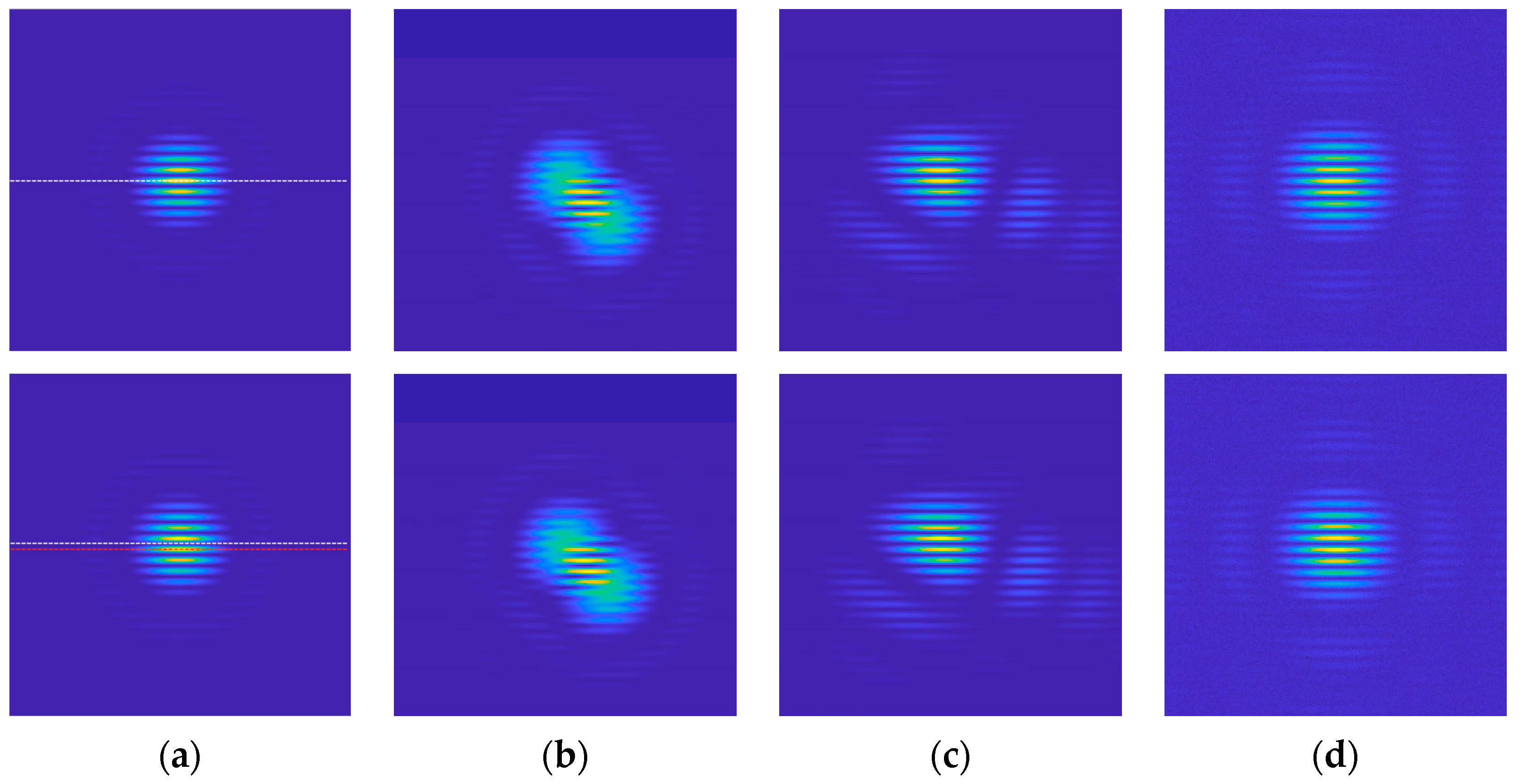Figure 3 shows the intensity diffraction images obtained under four conditions: (1) with piston error only, (2) with tip-tilt error, (3) with Zernike aberrations of the 4th to 11th order, and (4) with noise. It is observed that as the piston error varies, the position of the diffraction spot maxima shifts, as shown in Figure 3a. Specifically, when the piston error is 0, the intensity maximum aligns with the white dashed line, and as the piston error increases to 0.35λ, the intensity maximum moves to the red dashed line. This shift demonstrates the one-to-one correspondence between the diffraction pattern and the piston error. A dataset is then constructed based on the mapping relationship between image intensity and piston error, allowing the neural network to learn the correspondence between them.

2.3. Neural Network Model

Convolutional neural networks (CNNs) are a class of deep learning models particularly well-suited for processing data with a grid-like structure, such as images. CNNs can automatically extract spatial features from images by incorporating convolutional layers, pooling layers, and fully connected layers. Convolutional layers perform local perception operations on input data using convolutional kernels, gradually extracting features at different levels; pooling layers reduce the dimensionality of the data through downsampling while retaining essential information; fully connected layers use the extracted features for final classification or regression tasks. Deeper network architectures can extract more complex image features, but they also require longer training time and higher-performance computing resources.

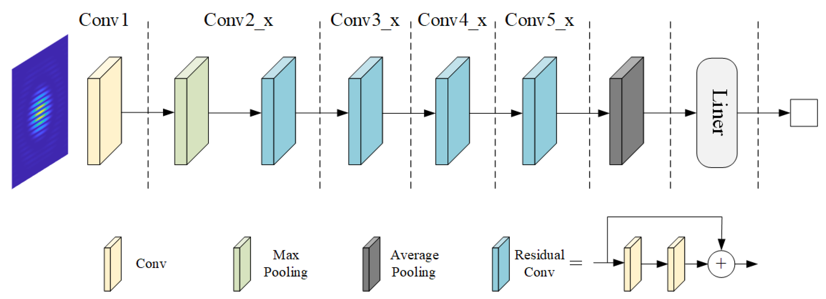
Based on multiple experiments, this study selected ResNet-18 as the foundational architecture of the network. This choice was made to balance performance and computational efficiency, as ResNet-18 can maintain accuracy while reducing training time and computational resource requirements. Multiple attempts were made to modify the network structure and associated hyperparameters based on ResNet-18, ultimately determining the optimized network architecture shown in Figure 4. Through these adjustments, the network demonstrated excellent performance in image feature extraction and piston error detection tasks.

The network primarily consists of four parts: convolutional layers, pooling layers, residual modules, and fully connected layers. The input to the network is a single-channel grayscale diffraction image of size 224 × 224. It first passes through a convolutional layer with a 7 × 7 kernel, reducing the image size to 112 × 112. This is followed by a pooling operation with a 3 × 3 pooling kernel, further reducing the image dimensions to 56 × 56. The network includes four residual modules, each composed of two residual blocks, and each residual block contains two convolutional layers. Through successive feature extraction, the image size is reduced to 14 × 14 with 16 convolutional kernels, while the number of output channels increases to 512. Next, the network performs global average pooling, transforming the output into a 1 × 1 × 512 tensor. Finally, a fully connected layer produces the regression prediction result. Since the piston error is a single scalar value, the output of the fully connected layer is set to 1 × 1. This structural design fully leverages the feature extraction capabilities of convolutional neural networks while preserving the feature propagation ability of deep networks through residual modules, providing a solid foundation for accurate piston error prediction.

We incorporated L2 regularization into the network to prevent overfitting during training. By adding a penalty term to the original loss function, this approach is formulated as follows:

$${\mathcal{L}}_{total}(W)=\mathcal{L}(W)+k\cdot {‖W‖}_2^2$$

(6)

where $W$ represents the weight matrix of the model, ${\mathcal{L}}_{total}(W)$ is the total loss function after adding the regularization term, $\mathcal{L}(W)$ is the original loss function, which is Mean Squared Error (MSE) loss in our regression task, $k$ is the hyperparameter for regularization strength that determines the influence of the regularization term, and ${‖W‖}_2^2$ denotes the squared L2 norm of the weight matrix $W$.

2.4. Network Training

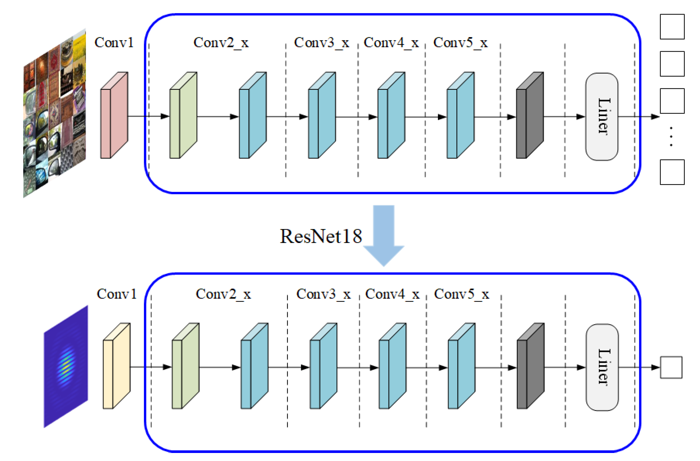
The ResNet-18 pre-trained model was trained on the ImageNet dataset, which contains tens of millions of images. In this study, while retaining the pre-trained parameters of the residual modules and pooling layers, the modified parts of the network, including the weights of the first convolutional layer and the weights and biases of the fully connected layer, were retrained, as shown in Figure 5. During training, we introduced the Kaiming initialization method to prevent vanishing or exploding gradients, which are common issues in deep networks using ReLU activation functions. This strategy helps ensure stable training and enhances the model’s ability to optimize key parameters for the specific task. By combining this approach with the pre-trained model’s feature extraction capabilities, we aim to improve the prediction accuracy and stability of the network.

The core idea of Kaiming initialization is to ensure that the variance of the input and output remains consistent across each layer. For networks using the ReLU activation function, the weights $W$ should satisfy the following condition:

$$W ~ \mathcal{N}(0,{\displaystyle \frac{2}{n}})$$

(7)

where $W$ represents the elements of the weight matrix, $\mathcal{N}(0,{\displaystyle \frac{2}{n}})$ denotes a normal distribution with a mean of 0 and a variance of ${\sigma }^2$, and n is the number of neurons in the previous layer. This initialization method is based on the characteristics of the ReLU activation function, where the output is the non-negative part of the input, and zeros out half of the input (the part where the input is less than zero). Therefore, a factor of 2 is multiplied to compensate for the attenuation of the signal.

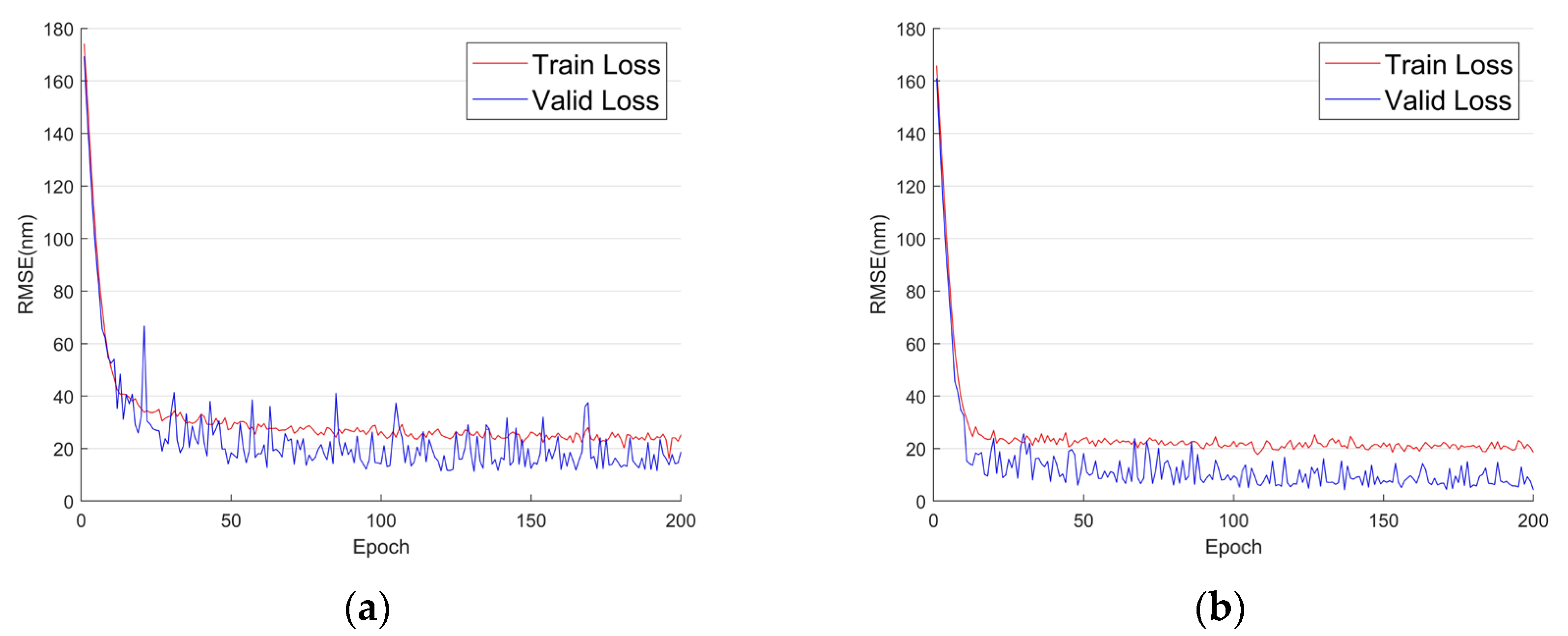
During training, the following hyperparameters were set: a batch size of 64, a learning rate of 0.001, and an L2 regularization coefficient of 0.001. The optimizer used was the Adam algorithm. The input images were 224 × 224 single-channel grayscale images. The hardware platform used for training included an Intel (R) Core (TM) i7-13700H CPU and an NVIDIA GeForce RTX 3050 GPU, with a software environment of Python version 3.11.5 and PyTorch version 2.1.2. Considering only the piston error, 10,000 diffraction images were randomly generated within the ranges of [−0.5λ, 0.5λ] and [−0.48λ, 0.48λ], with 8000 images used for training and 2000 for validation. The network was trained for 200 epochs, and the root mean square error (RMSE) during the training process is shown in Figure 6.

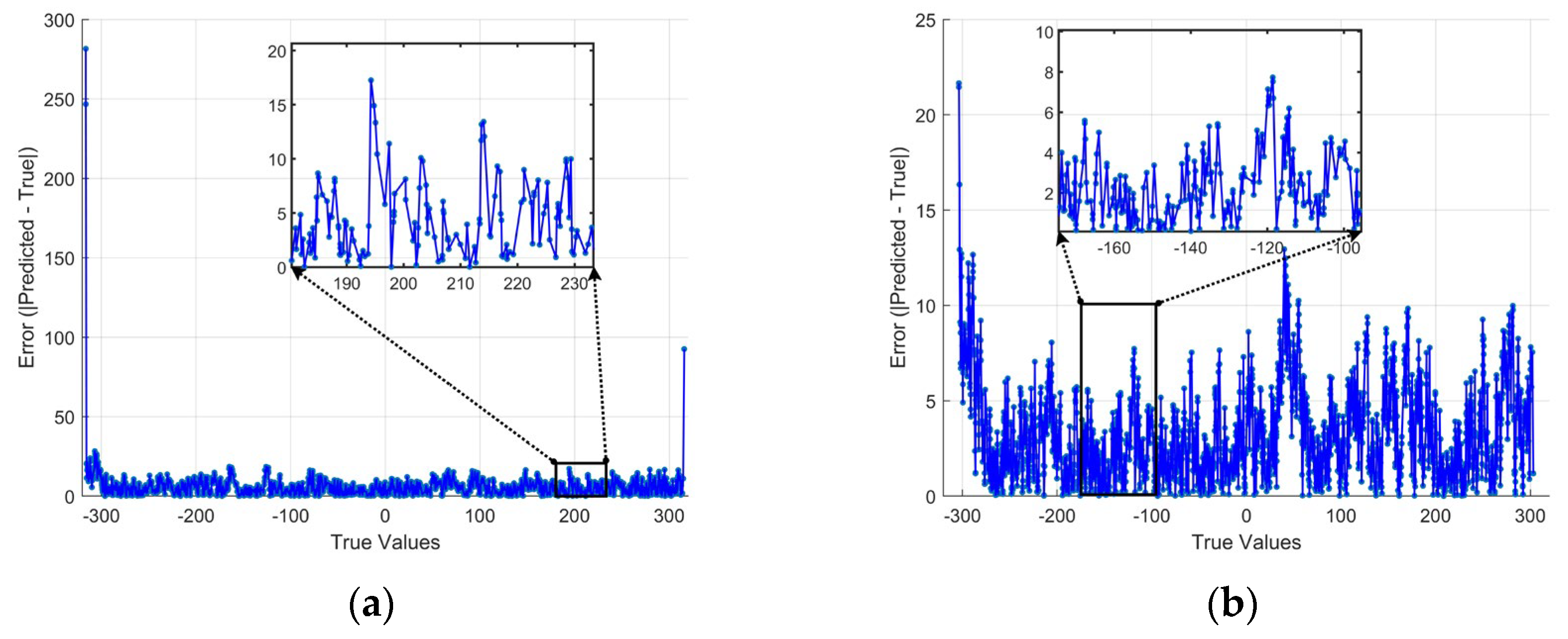
The performance of the trained model on the validation set was evaluated and compared in Figure 7. When the piston error was within the interval [−0.5λ, 0.5λ], the model achieved a minimum root mean square error (RMSE) of 11.2 nm (0.0177λ). Within this range, the prediction results for the piston error of 2000 diffraction images showed that the absolute error between the predicted and true values was primarily within 15 nm. When the piston error was within a smaller interval [−0.48λ, 0.48λ], the RMSE further decreased to 4.2 nm (0.0066λ). In this case, the absolute error between the predicted and true values for 2000 diffraction images was mostly within 5 nm. Notably, the anomalies observed near the edges of the larger interval were not caused by the dataset [24]. When the detection range was reduced to [−0.48λ, 0.48λ], the network maintained a high level of detection accuracy. Further narrowing of the range did not yield significant improvements in accuracy. Therefore, in this study, the subsequent piston error detection was consistently performed within the [−0.48λ, 0.48λ] interval to ensure high precision.

3. Simulation and Analysis

3.1. Robustness Analysis of the Neural Network to Residual Tip-Tilt Errors

Equation (3) describes the expression for the phase difference between two sub-apertures when only piston error is present. When there is a tip-tilt error around the x-axis or y-axis between the two segmented mirrors, the phase difference $∆\phi$ is

$$∆\phi ={\phi }_2-{\phi }_1={\displaystyle \frac{2\pi }{\lambda }}\cdot \{OPD+[\alpha (x-x_2)+\beta (y-y_2)]\}$$

(8)

where $\alpha$ and $\beta$ are the relevant gradients of the sub-apertures in the x and y directions, respectively. $(x_2 , { y}_2)$ represents the center coordinates of the second sub-aperture. $\alpha (x-x_2)$ and $\beta (y-y_2)$ denote the tilt phases induced by the tilt angles $∆{\theta }_x$ and $∆{\theta }_y$, respectively, as shown in Figure 8.

The robustness of the trained neural network model was analyzed under the presence of tip-tilt errors of 0.1λ, 0.2λ, and 0.3λ added to the apertures. Figure 9 shows the performance of the network model on the test set, illustrating the distribution of residual errors between the predicted and true values for 2000 test images. Figure 9a–c correspond to cases with tip-tilt error along the x-axis only, along the y-axis only, and equal tip-tilt errors along both the x- and y-axis, respectively. Compared to the case with equal tip-tilt errors along both axes, the network’s prediction accuracy decreases and residual error increases when tip-tilt error exists along only the x- or y-axis. This is caused by the elongation of the intensity peak on one side of the diffraction image. Nevertheless, the network still demonstrates good robustness in the presence of tip-tilt errors. With tip-tilt errors equal along both the x- and y-axis, when a tip-tilt error of 0.1λ exists between the two segmented mirrors, the model maintains high prediction accuracy, with 95.2% of the data having prediction errors within 5 nm. Even when the tip-tilt error increases to 0.2λ, the model’s performance remains robust, with 79.7% of the test set data showing prediction errors within 5 nm. Furthermore, when the tip-tilt error reaches 0.3λ, although the prediction errors increase, a significant proportion of the data (66.5%) still has errors within 5 nm, and only a small fraction (3.3%) shows prediction errors in the range of 10–15 nm, with no data exceeding the 15 nm error interval. These results indicate that the trained network model exhibits strong robustness in handling varying degrees of tip-tilt errors and can effectively predict piston errors while maintaining high prediction accuracy even in the presence of substantial tip-tilt errors.

3.2. Robustness Analysis of the Neural Network to Wavefront Aberrations

Wavefront aberration refers to the deviation between the wavefront formed by a spherical wave emitted from a point source after passing through an optical system and an ideal spherical wave. Aberrations can be expressed as a wavefront $W$ in units of wavelength. Given a determined mode, any arbitrary wavefront can be represented in the form of Zernike polynomials:

$$W\left(r,\theta \right)=\sum _{i=1}^{\infty }{a}_i{Z}_i(r,\theta )$$

(9)

where $a_i$ represents the coefficient of the i-th Zernike polynomial $Z_i$.

$$Z_i\left(r,\theta \right)=\left\{\begin{array}{c}\sqrt{2\left(n+1\right)}{R}_n^m\left(r\right)G^m(\theta ), m\ne 0\\ R_n^0\left(r\right) , m=0 \end{array}\right.$$

(10)

where $R_n^m\left(r\right)$ and $G^m$ denote the radial factor and azimuthal factor of the Zernike polynomial, respectively.

$$R_n^m\left(r\right)=\sum _{s=0}^{(n-m)/2}{\displaystyle \frac{{\left(-1\right)}^s\left(n-s\right)!}{s!\left(\frac{n+m}{2}-s\right) !\left(\frac{n-m}{2}-s\right) !}}{r}^{n-2s}$$

(11)

$$G^m\left(\theta \right)=\left\{\begin{array}{c}\sin (m\theta ), i odd\\ \cos (m\theta ), i even\end{array}\right.$$

(12)

Zernike aberrations of the 4th to 11th order were introduced into the circular aperture to simulate wavefront aberrations in a real optical system, with coefficients set to 0.04λ, 0.05λ, and 0.06λ, respectively, to analyze the network’s robustness to different wavefront aberrations. Figure 10 shows the performance of the trained network model on the test set for 2000 images, illustrating the distribution of residual errors between the predicted and true values. When the incident wavefront has a wavefront aberration of 0.04λ, the model performs excellently on the test set, with 79.5% of the prediction errors within 5 nm. When the wavefront aberration increases to 0.05λ, 75.7% of the data still maintains errors within the 5 nm range. Even when the wavefront aberration is increased to 0.06λ, the model’s robustness remains strong, with 73.3% of the test set data having prediction errors within 5 nm. In the error range of [5 nm, 10 nm), the error proportion remains within an acceptable range, with only a small percentage of data (2.3% to 2.7%) showing prediction errors between 10 and 15 nm, and no errors exceeding 15 nm. These results indicate that the trained network model exhibits strong robustness in handling different levels of wavefront aberrations. Even in the presence of a certain degree of wavefront aberration, the model can accurately predict piston errors, demonstrating high reliability and adaptability.

3.3. Robustness Analysis of the Neural Network to Camera Noise

The diffraction images in the optical system are captured by a CCD camera, which inevitably introduces noise during the imaging process. The signal-to-noise ratio (SNR) is a crucial parameter for assessing signal quality, representing the ratio of the power of the useful signal to the power of the background noise, typically expressed in decibels (dB). The formula is given by

$$SNR\left(dB\right)=10\log {\displaystyle \frac{P_{signal}}{P_{noise}}}$$

(13)

where $P_{signal}$ represents the signal power, and $P_{noise}$ represents the noise power. A high SNR indicates good signal quality with minimal noise interference, whereas a low SNR suggests poor signal quality.

In this study, Gaussian noise levels of 30 dB, 40 dB, and 50 dB were introduced into the diffraction PSF images to simulate the effect of camera readout noise and to analyze and compare the detection accuracy of the neural network in the presence of noise. Figure 11 shows the performance of the trained network model on 2000 test images, revealing the distribution of residual errors between the predicted and true values. When the signal-to-noise ratio (SNR) is 50 dB, the detection accuracy of the network reaches 0.00743λ, with 72.1% of the prediction errors within 5 nm. As the SNR decreases to 40 dB, the detection accuracy slightly drops to 0.00916λ, but the network still maintains good performance, with 63.5% of prediction errors remaining within 5 nm. When the SNR further decreases to 30 dB, the detection accuracy is 0.01384λ; despite the decrease in accuracy, 42.5% of the prediction errors are still within 5 nm, and 28.1% are between 5 and 10 nm. Even at an SNR of 30 dB, the vast majority of prediction errors remain within a reasonable range, with only a small fraction (7.6%) reaching or exceeding 15 nm. Considering that the SNR of current CCD cameras is typically greater than 40 dB, this detection method is suitable for practical applications in real-world systems, meeting actual application requirements.

4. Discussion

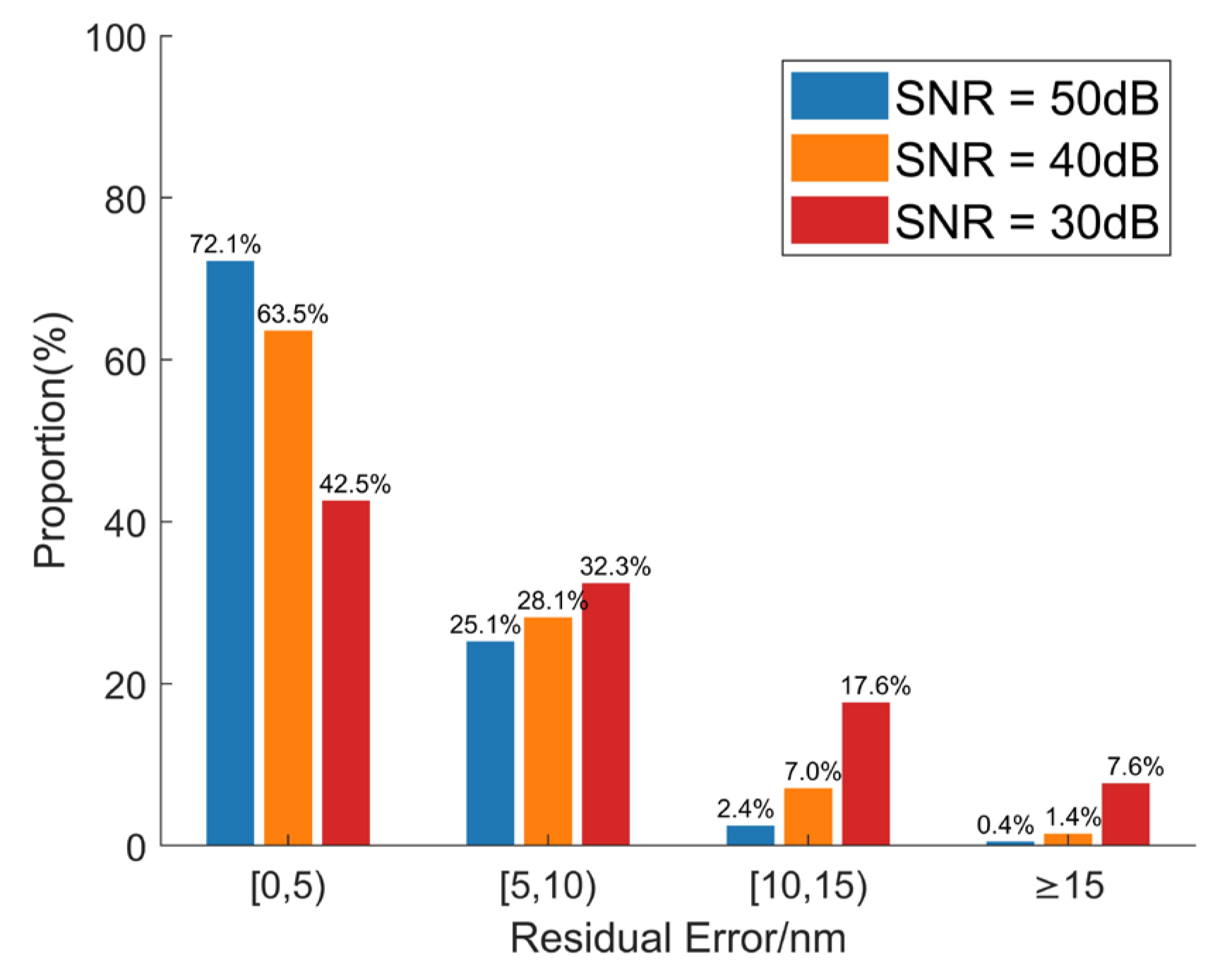
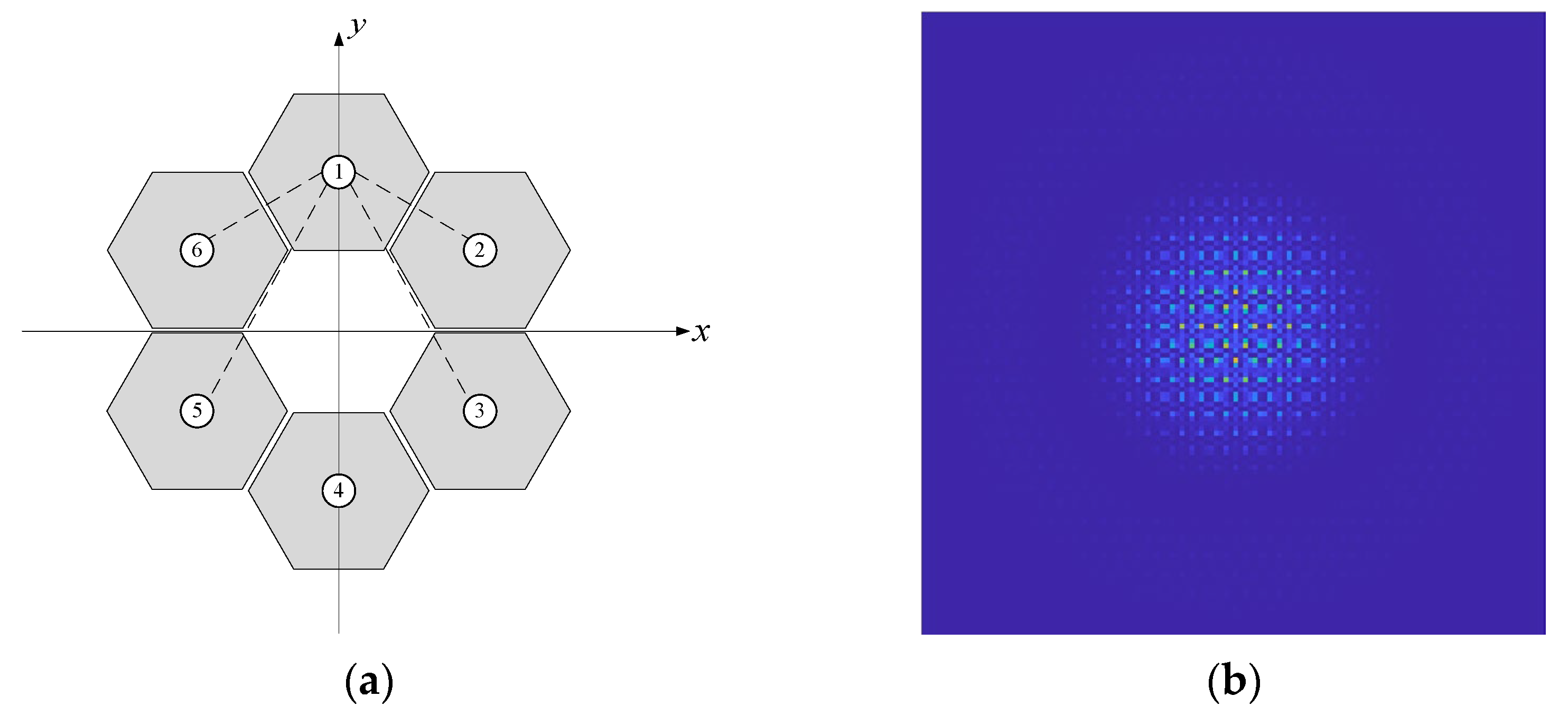
This section explores the application of a co-phase error detection method, based on far-field information and transfer learning, within multi-segment mirror systems. Using a six-segment imaging system as an example, the primary mirror structure and corresponding far-field diffraction pattern are shown in Figure 12. In this setup, Segment 1 is designated as the reference mirror, while the remaining five segments serve as test mirrors. System parameters are configured as follows: aperture diameter, D = 0.3 m, incident wavelength, λ = 632.8 nm, the focal length of the lens, f = 20 m, and the center coordinates (in meters) of the six mirror segments are (0, 1.32), (1.37, 0.61), (1.37, −0.61), (0, −1.32), (−1.37, −0.61), and (−1.37, 0.61). The corresponding far-field diffraction pattern is illustrated in Figure 12b.

Applying distinct piston values to the five test mirrors generates the respective far-field images. After constructing the dataset, model training is conducted using transfer learning. Notably, as there are five test mirrors, the neural network’s final output must be adjusted to accommodate five piston error values. In theory, the trained neural network should accurately predict the piston errors of the five test mirrors simultaneously. In our upcoming research, we will further assess the robustness of the proposed method within multi-segment mirror systems. Additionally, when scaling to systems with more mirror segments, several challenges are anticipated. First, the increase in segment count will require a significantly larger dataset to account for a higher-dimensional error space, which may introduce added complexity to both the data collection and model training processes. Furthermore, as the segment count rises, maintaining prediction accuracy across all segments might become more challenging, potentially necessitating enhanced model architectures or more sophisticated error correction algorithms. In this regard, we hypothesize the potential of exploring adaptive neural network structures and advanced transfer learning techniques to optimize the applicability and predictive performance of the method in higher-dimensional mirror configurations.

5. Conclusions

This study proposes a method for high-precision co-phasing detection of segmented mirrors using far-field information and transfer learning, based on the principle of double-aperture Fraunhofer diffraction. By modeling the optical system of the two submirrors, the impact of co-phasing errors on the performance of segmented mirrors was analyzed in detail, and a corresponding dataset was constructed within the range of [−0.48λ, 0.48λ]. The traditional neural network ResNet-18 was optimized using a transfer learning strategy, retaining some of its pre-trained parameters and retraining it on the constructed dataset. The trained network model demonstrated excellent detection accuracy, achieving 0.0066λ. Furthermore, the robustness of the convolutional neural network in co-phasing detection was validated through simulations under various error conditions. The results show that the method has good generalization capability, maintaining high detection accuracy even under different types and magnitudes of errors.

Compared to traditional optical methods, the co-phasing detection method based on far-field information and neural networks offers significant advantages. Firstly, this approach simplifies the measurement process and reduces data processing time, as the network can achieve high-precision detection of co-phasing errors in segmented mirrors using only a single frame of a far-field diffraction image. Secondly, neural networks exhibit strong robustness and adaptability, effectively predicting co-phasing errors even when processing noisy data in complex environments. Moreover, compared to other deep learning-based methods for piston error detection, this study introduces a transfer learning strategy, which ensures high accuracy while avoiding the complexity of building a neural network from scratch, thereby enhancing the method’s practicality and efficiency in real-world applications. The application of this proposed method to multi-segment mirror systems will be further explored in our subsequent research.