1. Introduction
Rotating laser beams became known after works [
1,
2,
3,
4]. It was shown in [
1] that rotating laser beams can be formed as an axial superposition of Laguerre–Gauss beams with certain numbers. In [
2,
3], rotating laser beams were experimentally formed as a superposition of Laguerre–Gauss beams using a Wolaston prism in a laser cavity [
3] and a diffractive optical element (DOE) [
2]. In [
4], rotating laser beams were also experimentally formed using DOEs, but these beams were a superposition of diffraction-free Bessel beams. In [
5], a spiral conical beam was studied; it was formed using a DOE with transmission exp(−
iα
rφ), where (
r,
φ) are the polar coordinates in the beam’s cross-section. In [
6], a two-lobe rotating beam consisting of two Laguerre–Gauss beams with different wavelengths was observed. Methods for increasing the formation efficiency of two-lobe rotating beams were considered in [
7,
8]. The formation efficiency of 57% was achieved in [
8]. In [
9], the orbital angular momentum of rotating beams, which are a superposition of Bessel–Gaussian beams, was analyzed, and the rotation speed of such beams was measured in [
10]. It was shown in [
11] that rotating laser beams can have zero orbital angular momentum. In [
12], laser beams with four rotating lobes in their cross-section were formed. Rotating laser beams are used to increase the longitudinal resolution of optical microscopes. For example, in [
13], a three-dimensional localization of an individual fluorescent molecule with a resolution of several nanometers was obtained using a rotating two-petal laser beam. In [
14], a second-order spiral zone plate was utilized to determine the diffusion parameters of fluorescent microspheres that are 100 nm in diameter. In [
15], a two-lobe rotating beam was formed by a meta surface with an efficiency of 70%. A two-lobe rotating beam was also been employed in [
16] for the three-dimensional localization of quantum dots with a resolution of about 10 nm. Additionally, a two-lobe rotating beam was formed in [
17] using a second-order spiral axicon. In all the works listed above, the angular velocity of the rotation of the beams in the cross-section did not exceed 50 deg/μm.
In this work, a three-petal rotating laser beam formed using a third-order spiral zone plate (ZP) is considered. Three local intensity maxima are formed in the beam that passed the ZP. If the ZP is displaced along the optical axis, then these three local intensity maxima will rotate around the optical axis. If we measure the rotation angle of the three-petal intensity distribution using a CCD camera, then we will be able to determine the shift of the ZP. By placing between the CCD camera and the ZP a thin film, it is possible to determine its thickness (or the change in thickness) by measuring the rotation angle of the three-petal beam. By shifting the film across the optical axis, one can measure the microrelief (thickness change) of the film over the cross-section by measuring the rotation angle of the three-petal beam. If a thin cuvette is placed between the ZP and the CCD camera, where a liquid flows, then utilizing the rotation angle of the three-petal beam, the refractive index of the liquid (or rather, the change in the refractive index), can be measured. In addition, if a thin plate placed between the ZP and the CCD camera is tilted by a small angle around an axis perpendicular to the optical axis, this tilt angle can be evaluated utilizing the angle of rotation of the three-petal beam. Note that the angular velocity of an intensity distribution rotation is shown in this work to be approximately 136 deg/μm, which is almost two times higher than in similar works on determining the 3D coordinates of nanoobjects [
13,
16]. For example, in [
13], the angular rotational velocity of the two-lobe intensity pattern was 45 deg/μm.
2. Theoretical Background
The theory of rotating optical vortices makes it possible to determine the rotation angle and relate it to the distance propagated by the laser beam [
11]. Taking into account that the distance propagated by light per time is also related to the parameters of the medium, particularly the refractive index, it becomes clear that the rotation angle can be related to the characteristics of the medium. Below, we will demonstrate how the angle of rotation of the generated intensity distribution can be used to measure characteristics such as a small shift, the thickness, the refractive index, and the tilt angle of thin films. It should also be mentioned that the theory can be applied not only in the classical case of superposition of optical vortices with different topological charges but also in the case of plane wave diffraction on a spiral axicon [
17]. However, the petal laser beam can also be formed using a spiral ZP [
18].
Let us compare the rotation velocity of the intensity lobes after the spiral axicon [
17] and the spiral ZP.
The transmission function of the phase spiral ZP has the following form:
where (
r,
φ) are polar coordinates in the plate plane,
m is an order,
k is a wave number of the light with the wavelength
λ, and
f is the focal distance of the parabolic lens. We can derive the transmission function of the binary amplitude spiral ZP from Equation (1):
where
is a sign function.
For a binary spiral axicon [
17], the transmission function is as follows:
where α determines the numerical aperture of axicon (NA = sin
α).
The rotation velocity of an
m-lobe optical vortex after an axicon (3) with a period
T was shown in [
17] to be as follows:
where Δ
φ is the angle of rotation of the intensity pattern when changing the distance Δ
z along optical axis. The rotation velocity of the intensity lobes after the focus of the spiral ZP in (1) can be rewritten as follows:
where
N is the number of the
N-th ring of the ZP. In the comparison of (4) and (5), we see that in both cases, the rotation velocity is constant (the tilt angle changes linearly with the distance) and depends inversely on the spiral number
m. Therefore, the rotation velocity in both cases is less for the spiral element with a higher
m. The minimum axicon period in (4) can be equal to the wavelength
T = λ. In our investigation, we proposed that the focal length in (5) equals to the wavelength
f = λ. In this case, the velocity (5) will be higher than the velocity (4) in
times. The use of the ZP instead of the axicon reduces the distance along the optical axis at which the beam rotates by the same angle. That is, a high numerical aperture and a short focal length of the ZP enable an increase in the angular velocity of the intensity distribution rotation by more than two times, relative to a spiral axicon [
17]. With a higher rotation speed, the reference beam formed by a spiral ZP, in contrast to the beam formed by a spiral axicon [
17], will make it possible to determine the characteristics of thin films more accurately. In view of this, in our work, we proposed an optical sensor technology based on a spiral ZP.
3. Optical Scheme of Measurements
In our measurement method, we propose a spiral binary amplitude Fresnel zone plate (2) with a focal distance of
f = λ, where λ = 532 nm is a wavelength. The binary relief of the element is proposed to be manufactured in a layer of aluminum with a thickness of
h = 60 nm and deposited on a glass substrate. The numerical aperture of this ZP is close to 1. The fabrication of an amplitude ZP using electron lithography technology is simpler than that of a phase ZP [
19]. However, the rotation of intensity maxima and its velocity are the same for both amplitude and phase zone plates.
The optical shift sensor works as follows (
Figure 1a): A linearly polarized Gaussian beam emitted by the laser is expanded by a micro objective and collected by a spherical lens onto the surface of the spiral ZP. In the transmitted beam, three local intensity maxima are formed at some distance along the optical axis behind the ZP (
Figure 1b). If the CCD camera is moved along the optical axis, then the intensity distribution in the beam’s cross-section, in the form of several petals, will rotate around the optical axis. By measuring the rotation angle of the petals, the shift of the ZP or CCD camera can be obtained. Light from circles of different radii propagates to different output transverse planes, causing the intensity petals to rotate. Additionally, because of the helicity of the ZP, branches of the spiral in different places intersect circles of different radii. Thus, the produced intensity maxima are visible and rotate until the ZP begins to work as a whole, that is, when light from each ZP point comes to each point of the beam.
As will be shown below, the use of a short-focus ZP instead of an axicon [
17] makes it possible to increase the sensitivity of the displacement measurement method by several times. In addition, as it will be shown below, using a third-order spiral, in contrast to the second-order axicon used in [
17], makes it possible to increase the accuracy of measuring the rotation angle by averaging over three lobes. At the same time, the magnitude of the order of the ZP is not so significant. You can use ZP or the second or third order.
4. Estimation of the Rotation Velocity Using Numerical Simulation
In this section, using numerical simulation, we find the dependence of the rotation angle on the shift distance of the output plane. We consider the ZP with
m = 2,
m = 3, and
m = 4. The size of the ZP in the simulation is chosen to be 8 × 8 µm. The relief pattern of the spiral ZP for
m = 3 is shown in
Figure 2. The simulation is carried out using the FDTD method implemented in the FullWave (RSoft) software package 2018.03, 64-bit; the simulation grid in all three coordinates is λ/30. The incident wave is a Gaussian beam with a waist radius of
w = 3 μm, limited by an aperture with a radius equal to 4 μm.
Figure 3a demonstrates dependences of the tilt angle
φ of the intensity maxima on the observation distance from the relief along the optical axis
L (μm) in free space calculated for different orders
m.
The plot of the tilt angle
φ is seen from
Figure 3a to have the longest length for the case
m = 3, up to the value
L = 2.5 μm. It is seen that the higher is the ZP order
m, the lower is the rotation rate of the intensity maxima. The angular velocity is the highest for the order of the ZP
m = 2, but starting from the distance
L = 2 μm, the intensity maxima merge, which makes it difficult to recognize the angle
φ (
Figure 3c). The simulation for
m = 3 shows that before the focus, three intensity lobes had not yet formed. Only after the focus (
L =
f = λ = 0.532 μm) do they appear and rotate up to a distance of approximately 2 μm (
Figure 3a). After this distance, the intensity pattern more and more resembles an inhomogeneous light ring, and three local maxima can no longer be distinguished. At the same time, the contrast of images for values
m > 3 or
m < 3 is worse, as can be seen from the example in
Figure 3b,c. For
m > 3 (for example,
m = 4), an intensity peak appears on the optical axis, and all the intensity maxima rotating around the optical axis become closer to each other. Since that, we simulate a ZP with the order
m = 3.
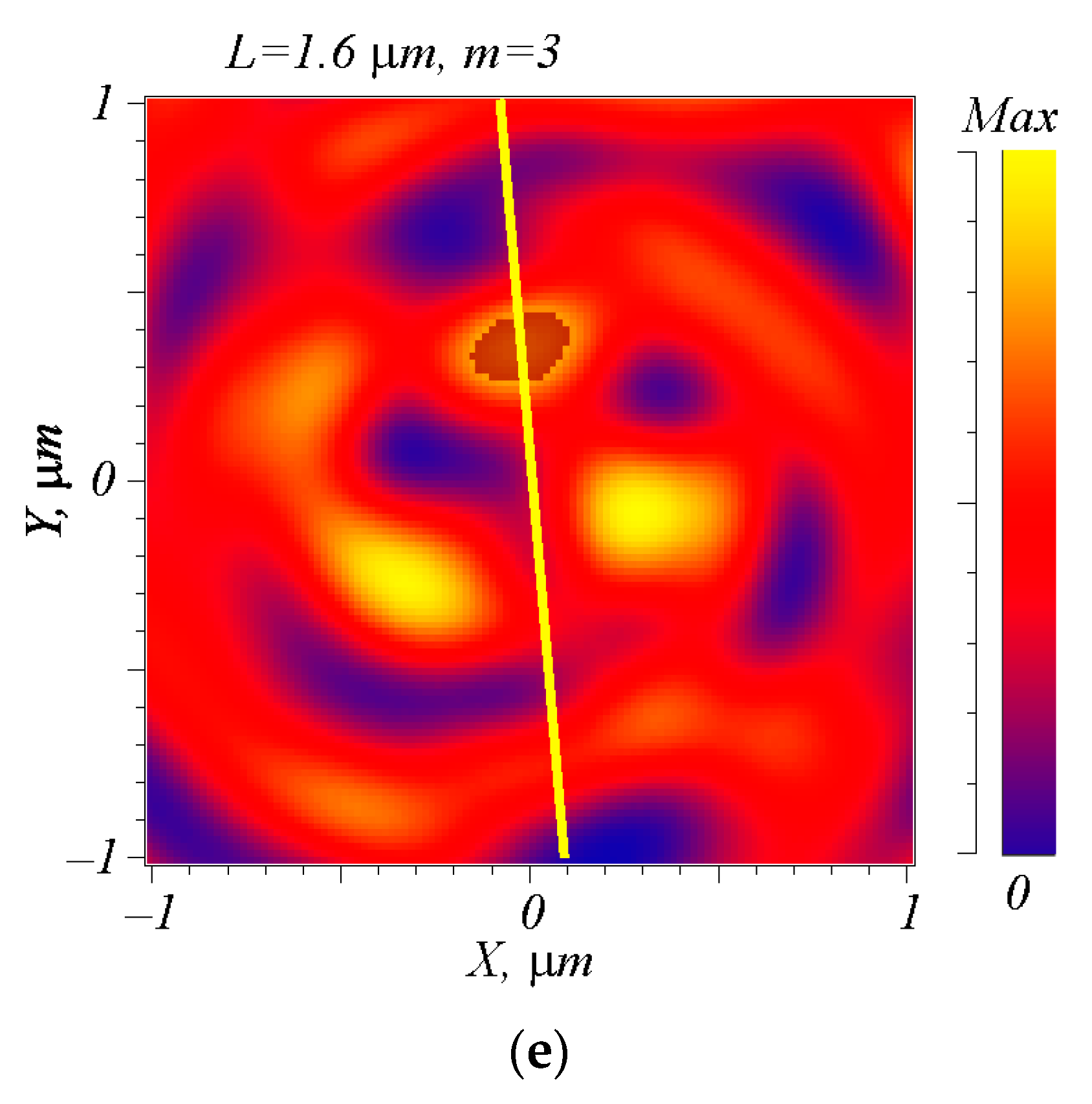
The rotation angle of a single intensity maximum (it is indicated in
Figure 3d by a blue arrow) is determined as follows: First, three points with the maximum intensity in the beam’s cross-section are found. Then, a line connecting the selected intensity maximum with the middle of the segment connecting the centers of the other two maxima is found. This line is shown in
Figure 3 in yellow. Next, the angle of this yellow line relative to the horizontal
x-axis is found. In
Figure 3d, points (indicated by the blue arrow) are used to obtain the average coordinates of the intensity maximum, so points greater than 0.85 of the local intensity maximum are utilized. The averaging helps to obtain more accurate positions of peaks.
At a distance of about 2 µm behind the focal plane (
f = 0.6 µm), the rotation angle changes from −50° to 210° (the rotation angle range is about 260°), as shown in
Figure 3a. The “velocity” of the intensity distribution rotation is 136 deg/µm, which means it takes 2.63 µm to make a full turn. For example, for the case of
m = 2, it is 211 deg/μm, and for
m = 4, the velocity is 102 deg/μm. Examples of evaluations of the rotation angle of the intensity maximum at
L = 1.3 µm and
L = 1.6 µm are shown in
Figure 3d,e (ZP with
m = 3). The rotation angle relative to the
x axis is 49.3° for
L = 1.3 µm and 95° for
L = 1.6 µm. The calculation is performed in an automatic mode with a shift of the observation plane by 0.1 μm, and the intensity is taken into account greater than 0.8 of the maximum. Note that, in this case, the rotation velocity of the beam produced by ZP with
m = 2 is almost 2.5 times higher than in [
17], where a spiral axicon with
m = 2 is proposed. The simulation shows that for the chosen parameters, the rotation can be distinguished with a resolution of 1°. This means that the minimum shift possible to measure this sensor is 1000/136 ≈ 7 nm. The rotation of the intensity pattern in
Figure 3 is counterclockwise. This is because the order of the spiral in
Figure 2 is positive (
m > 0). If the spiral order is negative (
m < 0), then the intensity lobes would rotate clockwise with increasing
L.
The contribution to the intensity at a distance of up to 2 μm from the ZP is seen from
Figure 3b,c to be made by the first 1–2 rings of the ZP. If we assume that
N = 1.5, then the square root will be equal to
= 1.22 and the velocity (5) will be equal for our case (
Figure 3):
rad/μm = 137.5 deg/μm. This value is slightly higher than the simulation result (136 deg/µm). It is seen from
Figure 3a that with an increase in the helix order
m, the velocity decreases according to Formula (5). Moreover, the ratio of the velocities obtained from
Figure 3a is exactly equal to the ratio of the spiral orders: 211/136 = 3/2 and 136/102 = 4/3.
5. Simulation Results of the Thin Transparent Film’s Thickness Measurement
Utilizing the rotation angle, not only the shift of the ZP or CCD camera can be evaluated. In this section, we describe the accuracy of measuring the thickness of thin films achievable by this sensor. We assume that a thin dielectric film is placed between the spiral ZP (
Figure 2) and the observation plane (CCD camera in
Figure 1b). Then, the rotation angle of the three-petal intensity distribution will be proportional to the film’s thickness.
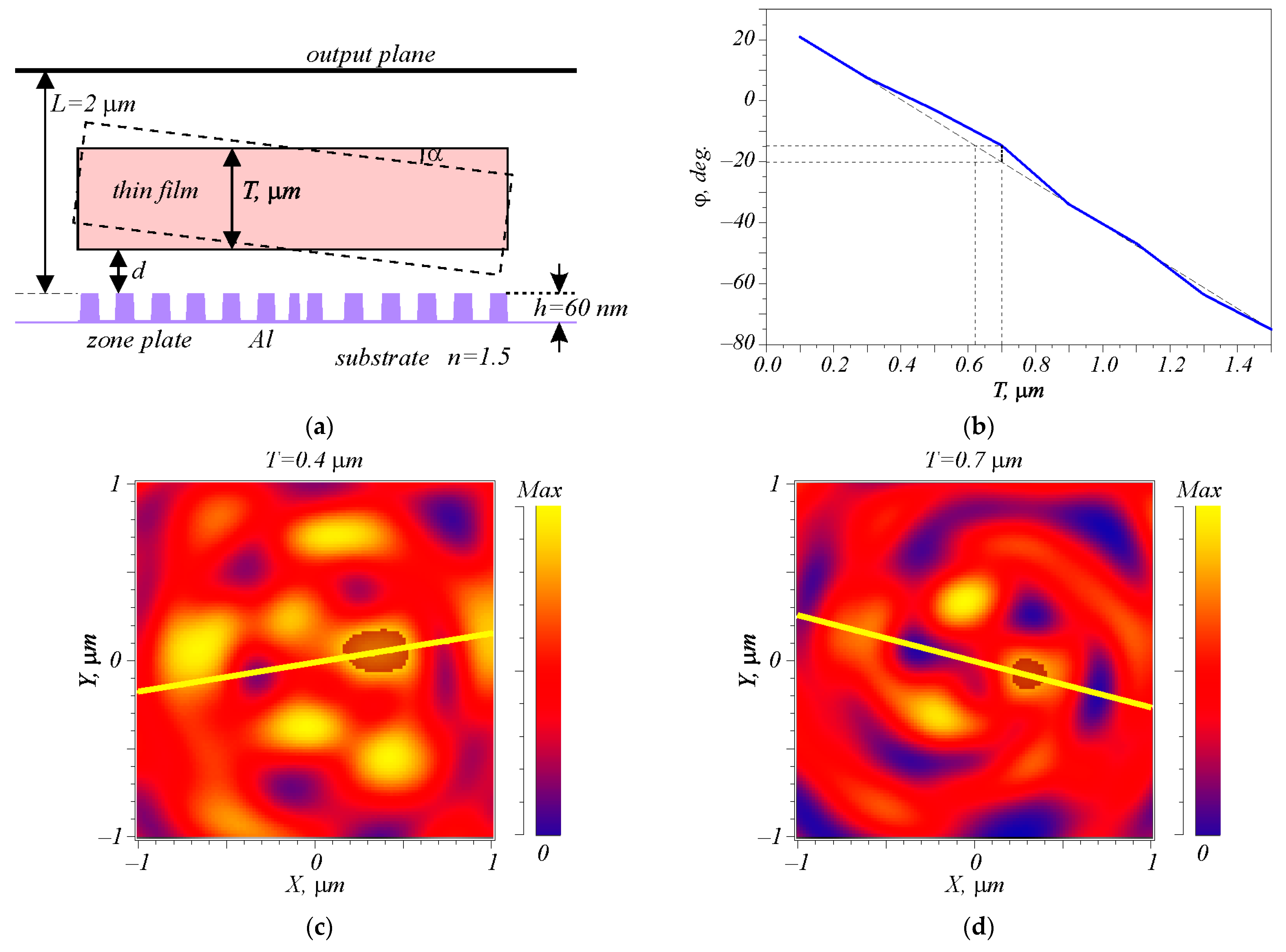
Figure 4 shows the simulation diagram (a) and the rotation angle
φ as a function of the film’s thickness
T (b).
Figure 4c,d shows the intensity distributions of the three-petal beam passed through the ZP (
Figure 2) for the thicknesses of the measured films (
Figure 4a)
T = 0.4 µm (
Figure 4c) and
T = 0.7 µm (
Figure 4d). The refractive index of the film is
n = 1.5; the distance between the film and the ZP is
d = 0.2 µm. The film’s thickness varies in the range from 0.1 to 1.5 µm with a step of 0.2 µm, and the film’s tilt angle α = 0. The output plane (CCD camera) is placed at a distance of
L = 2 μm from the upper edge of the ZP relief.
The simulation shows that an increase in the film’s thickness by 1 μm (
Figure 4b) causes the rotation of the intensity maxima by −68.5°, which is approximately two times less than in the case shown in
Figure 3a. This is explained by the chosen refractive index of the film, which leads the eikonal (phase delay) to slowly increase twice, relative to the thickness of the film. The rotation direction in this case is the opposite (
Figure 4b). This occurs because when rays fall to a medium with a higher refractive index, the angle of rays to the optical axis becomes smaller, and the focal length
f of the ZP increases by the value
T, which results in the intensity maxima rotation becoming slower (5). Because the rotation velocity in the medium is lower, the beam rotation angle at a distance of
L = 2 μm (
Figure 4a) is also smaller. Additionally, the thicker the film, the lower the rotation angle of the beam will be at the same distance. There is an effect of rotations in the opposite direction (clockwise). If the film’s thickness is fixed and shifted along the
z axis between the ZP and the CCD camera, then no rotation of the intensity maxima occurs.
There are two criteria for evaluating the quality of the measurement—the sensitivity of the method and the accuracy of the measurement. We obtain the rotation angle, utilizing averaging of points coordinates in a petal with intensity higher than a threshold (it equals 0.8 max); this method has very high sensitivity. This is demonstrated in
Table 1. In this case, the resolution in the output plane along the
x and
y axes coincides with the simulation grid and is equal to λ/30 = 0.0177 µm.
Table 1 shows the rotation angles
φ obtained for different film thicknesses
T.
It can be seen from
Table 1 that for the given simulation parameters, the change in thickness by 1 nm cannot be distinguished. This is because the simulation grid step along the
z axis has also been 0.0177 µm. That is, changes in the film’s thickness may not lead to a change in the simulation scheme, since the modeling grid is coarser. However, it has been shown that a change in the thickness by Δ
T = 3 nm can be detected by this method. To evaluate the accuracy of measuring the film’s thickness, the standard deviation of the difference between the resulting profile and the straight line closest to this graph (
Figure 4b, dotted line) has been calculated. The obtained standard deviation is σ = 2.39°, i.e., the root-mean-square error in evaluating the thickness is expected to be ±35 nm.
6. Simulation Results of the Thin Transparent Film’s Tilt Angle Measurement
In this section, we show that the optical sensor with a spiral ZP can evaluate the tilt angle α of a thin transparent film placed between the ZP and the CCD camera. The film turns around an axis perpendicular to the optical axis (
Figure 4a).
Figure 5 demonstrates the resulting rotation angle
φ of the three intensity maxima as a function of the tilt angle α of the film. The simulation parameters are as follows: the film’s thickness
T is 0.5 µm, the refractive index
n is 1.5, and the film tilt angle α varies from 0 to 7 degrees. The distance between the film and the ZP is increased to
d = 0.6 µm.
It follows from
Figure 5 that the rotation of the film, on the one hand, affects the accuracy of determining its thickness. A change in the angle α in the range from 0 to 7° leads to a rotation of the intensity maxima by 3°, which corresponds to increases in the maximum error in measuring the thickness of ±44 nm. However, on the other hand,
Figure 5 demonstrates that the optical sensor can measure the tilt angles of the film too. If the thickness of the film is known and is necessary to evaluate the tilt angle of the film, then according to the plot in
Figure 5, this method can measure the tilt angle in the range from 0° to 2° with an accuracy of 0.1°, or in the range from 3° to 7° with the same accuracy.
7. Simulation Results of the Thin Transparent Film’s Refractive Index Measurement
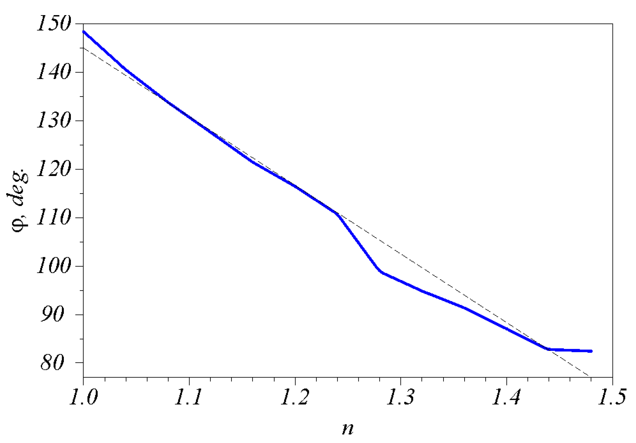
It is clear that a change in the refractive index of an object between the ZP and the CCD camera also introduces a difference in the eikonal of the light wave, and the output three-petal beam rotates. Therefore, this optical sensor can evaluate the refractive index of a thin film or liquid in a cuvette if its thickness is known. The dependence of the rotation angle of the intensity maxima
φ on the refractive index
n in the range from 1 to 1.5 for the film’s thickness
T = 0.5 μm is shown in
Figure 6.
It follows from
Figure 6 that increasing the refractive index by one results in decreasing the angle
φ by 141.7°. It also follows from
Figure 6 that if the refractive index increases by one or two tenths, then the focal length of the ZP almost does not change and the rotation velocity is approximately equal to the rotation velocity without the film (
Figure 3). However, since the speed of light inside the film is lower, the rotation angle of the beam in the output plane is smaller relative to the case without the film. Therefore, the rotation becomes clockwise (
Figure 6), in contrast to the case without the film (
Figure 3), where the rotation is anticlockwise. With a further increase in the refractive index of the film, the focal length of the ZP increases, and the rotation velocity decreases. Therefore, we do not show the plot for
n > 1.5 in
Figure 6. The dependence shown in
Figure 6 is not a straight line. The standard deviation between the obtained plot and the straight line (dashed line in
Figure 6) is 2.63°, which corresponds to the accuracy of determining the refractive index
n ± 0.019. However, the sensitivity of this method is better, and the minimal resolution in measuring the refractive index is Δ
n = 1/141 = 0.007.
8. Experimental Measurement of the Rotation Velocity
Previously, we made a second-order ZP. Therefore, we added this section to the comparison of the simulation and the experiment for a second-order ZP. We used electron beam direct recording technology and subsequent plasma etching a second-order helical ZP (
m = 2) with a diameter of 12 μm and a focal distance equal to the wavelength (
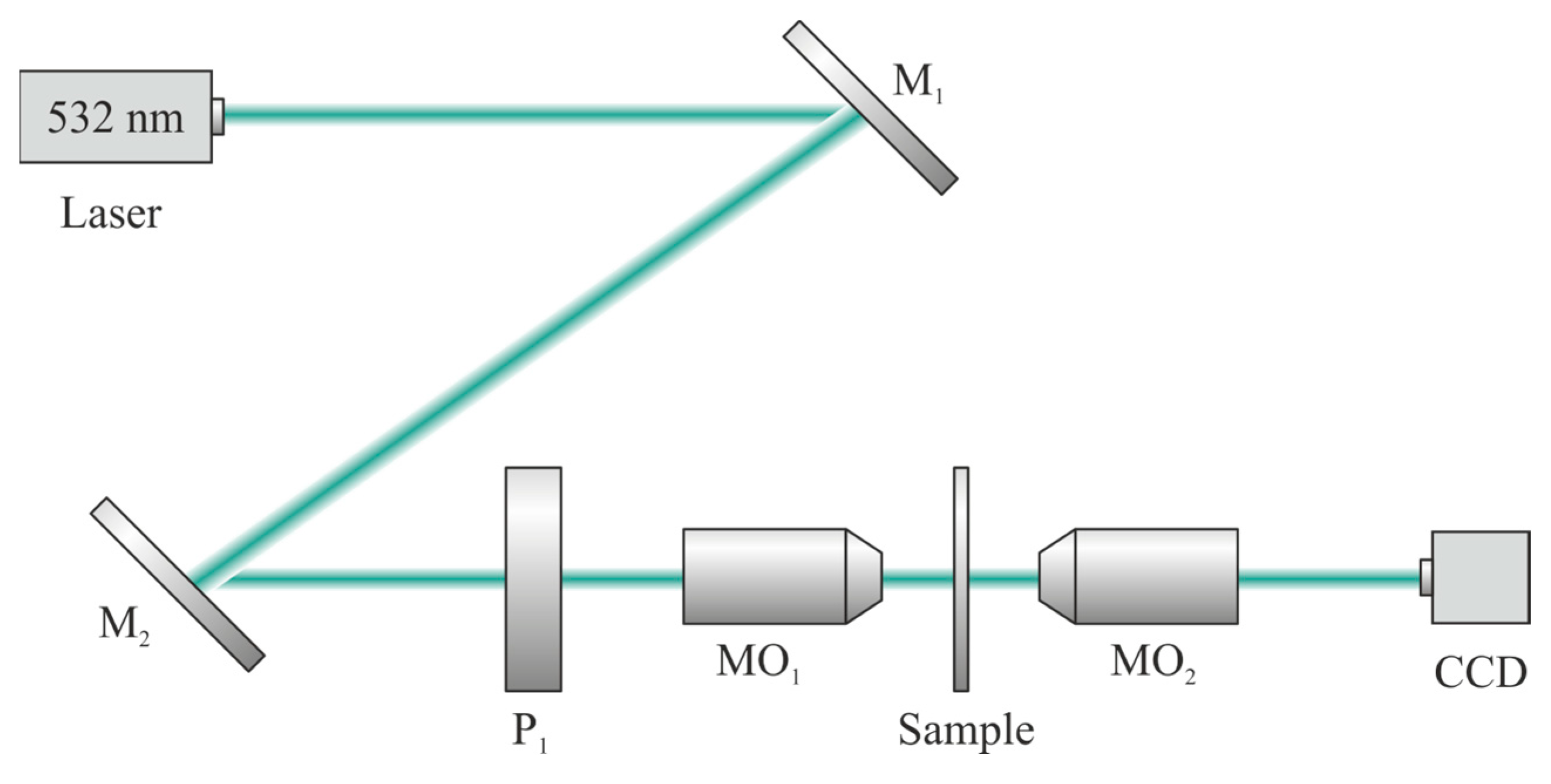
f = λ = 532 nm), which was fabricated in a thin film (60 nm) of aluminum deposited on a silicon substrate. The experimental setup (
Figure 7) included the following: a laser, a polarizer P
1, a micro-objective MO
1, focusing light on the ZP, and a micro-objective MO
2, depicting the focal plane on the CCD camera sensor. The light from the MGL-F-532-700 laser (λ = 532 nm) passed through the P
1 linear polarizer and was focused 4× by the Olympus RMS4X (MO
1) objective onto the investigated ZP (sample). Images of the transmitted beam were detected using a 100× Nikon objective (NA = 0.95) on a UCMOS10000KPA CCD camera. The camera was moved along the optical axis to register the rotation of the intensity lobes.
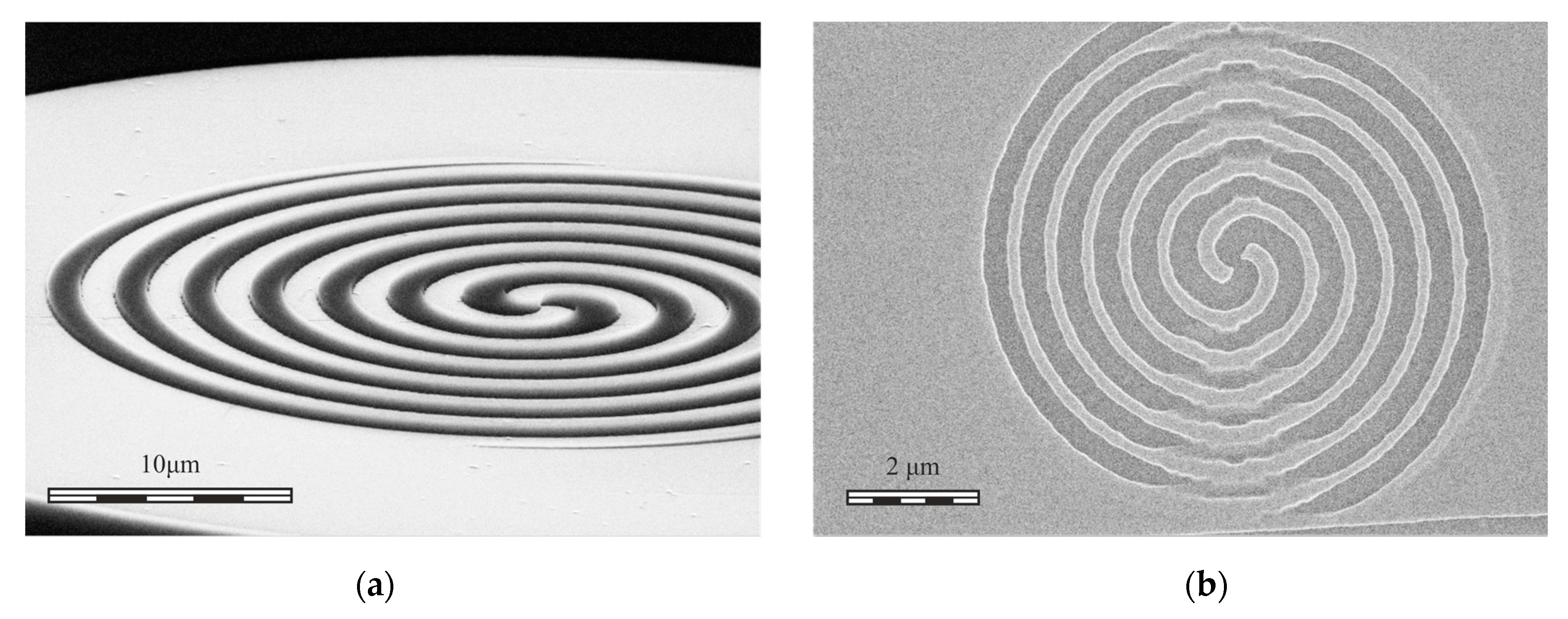
Images of a mask in a thin chromium film (45 nm) (a) and of the fabricated ZP in the thin aluminum film (b) derived by an electron microscope are shown in
Figure 8.
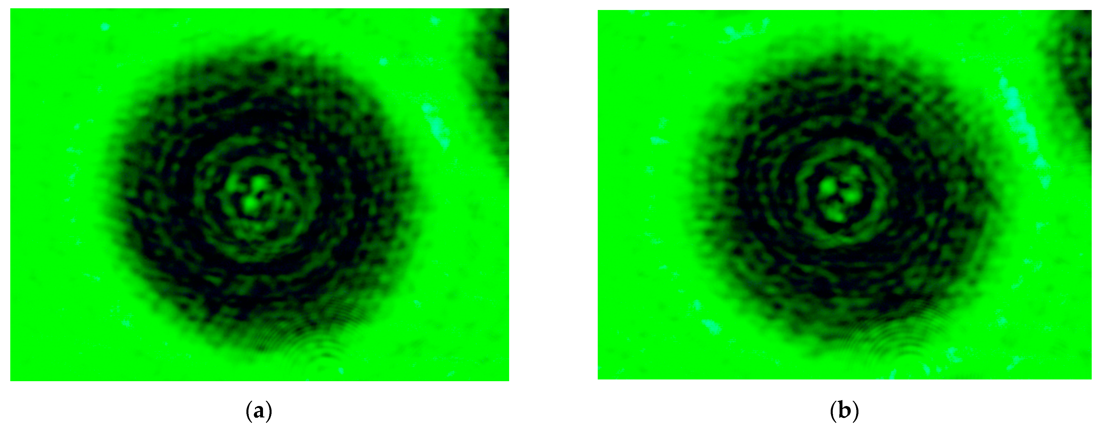
Figure 9 shows two intensity distributions recorded by the CCD camera at distances
L = 1.3 µm (a) and
L = 1.7 µm (b) after the ZP. Two intensity lobes are seen in
Figure 9 to rotate by almost 91° after 0.4 μm. It follows from these measurements that the rotation velocity of the intensity lobes is approximately 227.5 deg/μm. This is more than the velocity obtained by the simulation (
Figure 3a): 211 deg/μm. The error (about 7%) appears because of the accuracy of measuring the displacement of the CCD camera; this accuracy is about 0.1–0.2 μm.
9. Conclusions
Based on the FDTD method, a simple optical sensor methodology is developed. It can evaluate several parameters at once: a shift, a thickness or relief profile, a tilt angle, and a refractive index. Rotating laser beams containing a two-petal intensity distribution have been used for a long time to increase the longitudinal resolution of optical microscopes. The two-petal point spread function makes it possible to determine the three-dimensional position of an individual molecule or quantum dot with an accuracy of 10 nm–20 nm [
13,
16]. In this work, a rotating beam was generated using a light modulator. In order to miniaturize the optical sensor, in this paper, we propose using a microelement in the form of a third-order spiral binary amplitude zone plate with a high numerical aperture and a size of only 8 × 8 μm, made in a thin aluminum film 60 nm thick. It is shown that shifting the output plane by about 2 μm from the ZP surface results in an almost linear rotation of the three-petal beam by about 260° (
Figure 3a). The achieved angular rotation velocity of 130 deg/μm is more than two times higher than that achieved in similar works [
8,
13]. This paper also shows that if a thin film with a thickness ranging from 200 nm to 1400 nm is placed between the ZP and the output plane (CCD camera), then the change in the film’s thickness can be evaluated utilizing the rotation angle of the three-petal intensity pattern (
Figure 4b) with an accuracy of 35 nm. The minimum detectable change in the film’s thickness is 3 nm. This optical sensor (
Figure 1) is shown to make it possible to evaluate the refractive index of thin films if their thickness is known. In this case, the accuracy of determining the refractive index is 0.019. It can also measure the tilt angle α by several degrees with a thin transparent film. In this case, the accuracy is about 0.1°. Although this sensor methodology cannot achieve outstanding accuracy in measuring these values, it is based on a spiral zone plate, which is simple to fabricate. It is easy and quite multifunctional.


