Abstract
Single-pixel hyperspectral imaging (HSI) has received a lot of attention in recent years due to its advantages of high sensitivity, wide spectral ranges, low cost, and small sizes. In this article, we perform a single-pixel HSI experiment based on an untrained convolutional neural network (CNN) at an ultralow sampling rate, where the high-quality retrieved images of the target objects can be achieved by every visible wavelength of a light source from 432 nm to 680 nm. Specifically, we integrate the imaging physical model of single-pixel HSI into a randomly initialized CNN, which allows the images to be reconstructed by relying solely on the interaction between the imaging physical process and the neural network without pre-training the neural network.
1. Introduction
Hyperspectral imaging (HSI) is a new imaging technique developed in recent years to acquire spectral data cubes in scene space. It usually uses multiple well-defined optical bands in a wide spectral range to capture objects, so it contains a set of two-dimensional (2D) images at different wavelengths. Due to its spatial and spectral resolution, HSI is significantly useful and important for measuring scenes and extracting detailed information [1]. Over the past two decades, HSI has evolved from its original applications in remote sensing using satellites and airborne platforms to many scenarios including mineral exploration [2,3], medical diagnostics [4,5], environmental monitoring [6], etc. In general, dispersive optical devices, filters, and interferometers were used to separate the light-intensity information of different wavelengths in most of the existing HSI systems, which were measured and recorded by the array detectors. Specifically, dispersive spectral imaging technology uses prisms, gratings, and other instruments to achieve dispersion, which is relatively mature and widely used at present. Filter-type spectral imaging technology is mainly used for tunable filters, which have the characteristics of fast speeds and ease of use. Interferometric spectroscopy imaging techniques use an interferometric spectrometer to split the incoming beam in half, as well as vary their optical path differences to produce different interference intensities at each spatial point. Then, spectral information can be extracted by the Fourier transform of these intensities, measured by the array detector [7].
In HSI, it is usually necessary to acquire high-resolution images to distinguish the specific details of the scene, which inevitably requires the acquisition of a huge amount of data and increases the cost of processing and storage. Compressed sensing (CS) [8,9] has brought a new vitality to spectral imaging, which has boosted to produce a new field of compressed spectral imaging (CSI). CS shows that if the signal is sparse, the object images can be reconstructed from a number of samples far below the number required by the Nyquist sampling theorem. Specifically, the spatial and spectral information of the target scene can be retrieved from a small number of samples in CSI, which is based on the premise that hyperspectral data are redundant in nature. Using the theory of CS, multispectral images can be multiplexed together to reduce the required sampling rate () [10]. To date, several CSI schemes have been developed. Typical examples include the spatial–spectral coded compression spectral imager [11], coded aperture snapshot spectral imager [12,13], and dual-coded hyperspectral imager [14]. However, 2D detectors are used in most of these spectral imagers, which inevitably limits the spectral range of detection, reduces the efficiency of photon collection, and increases the cost [7,15].
It is gratifying that single-pixel imaging (SPI) [16,17] provides another promising solution for HSI, which uses a single-pixel detector (SPD) instead of traditional 2D detector arrays to capture the single-pixel bucket signals. The spectral images of the scene are recovered by various recovering algorithms using these bucket signals of different central wavelengths and a set of 2D modulated bases for the spatial light modulator (SLM), respectively. Therefore, it has lower cost, a wider spectral detection range and a higher photon efficiency [18,19,20]. In the past decade, SPI has achieved great success in various applications [21,22,23,24,25,26]. Many HSI schemes using SPD have been proposed [7,27,28,29,30,31,32,33,34,35,36,37], among which the CS-based algorithm is undoubtedly one of the most popular reconstructions to obtain reconstruction spectral images at a lower sampling number. However, these methods usually require a large number of iterative operations, which significantly increases the computational cost.
Recently, data-driven deep learning (DL) [38,39,40] has become another widely used reconstruction algorithm for single-pixel HSI which stems from DL’s proven power in solving various computational imaging inverse problems [41,42,43,44,45,46,47]. Unlike CS, DL-based methods do not require complex iterative operations, allowing higher-quality reconstructed images to be obtained at a lower SR. Although data-driven DL methods show excellent performance in single-pixel HSI, these methods require a lot of input and output data pairs to train the neural network. Therefore, these methods have inherent defects in generalization, interpretability, and model training time. One of the solutions is the recently proposed fusion of the physical process of imaging into a hand-crafted randomly initialized untrained neural network. Because there is no need to train neural networks on large datasets, this method has strong competitiveness in interpretability, generalization, and efficiency of time. Specifically, the idea of such an untrained neural network is derived from the deep image prior (DIP) theory proposed by Ulyanov et al. [48] in 2018, which states that the structure of a reasonably designed generator network has an implicit prior to natural images, so it is sufficient to capture a large number of image statistics before any learning. It has been reported that many targets of image reconstruction in optical imaging have been achieved by this method [49,50,51,52,53,54]. In general, the input to the network is just a set of one-dimensional optical intensity values collected by the SPD. The neural network weight and deviation parameters can be optimized to generate high-quality reconstruction images through the interaction between the neural network and the imaging physical model. A typical example is that a ghost imaging (GI) scheme using deep neural network constraint (GIDC) has been proposed in Ref. [50] to achieve a far-field super-resolution GI.
Inspired by the DIP and GIDC, this article proposes a single-pixel HSI scheme via untrained neural network constraints, which integrates the physical model of the single-pixel HSI into a randomly initialized convolutional neural network (CNN) to obtain high-quality reconstruction results without data training. Different from the GIDC, the differential bucket signals are fed into the network, which could greatly reduce the noise caused by the detector and the environment. A fuzzy reconstruction using CS is also fed into the network. With the interaction between the neural network and the imaging physical model, the deviation parameters of the network are constantly optimized, so as to obtain high-quality reconstruction results. Experimental results show that the proposed method has a better image quality, higher signal-to-noise ratio (SNR), and contrast, compared with CS.
2. Principle and Method
2.1. Experimental Setup
The experimental setup is sketched in Figure 1. A white light beam from a LED light source passes through a transmissive object and the imaging lens (f = 10 cm) in turn and then illuminates onto a digital micromirror device (DMD, V-7000, ViALUX), where the focal length of the imaging lens and the distances from the lens to the object and to DMD meets the Gaussian convex lens imaging formula. The Hadamard matrices based on the Haar wavelet transform (a value of “0” or “1”) [55]. Figure 1a were chosen as the modulation matrices, which are loaded in advance onto the DMD before the start of the experiment. One of the reflected light beams from the DMD that carries the information of the modulation matrices is collimated into a grating monochromator to be dispersed into the different spectral channels (Figure 1b). The SPD (DET36A2, Thorlabs) is set at the exit of the monochromator to capture a series of these channels’ bucket signals, which is then connected to an analog-to-digital converter (ADC) to be digitized. Finally, these digital signals are stored in a computer by a data acquisition card (DAQ, NI-6002) for reconstruction of the spectral data cube. In the following experiments, the modulation frequency of the DMD is set to 20 Hz while the acquisition card works at 1 kHz. That is, during an illumination time for each modulation, 50 digital data can be acquired and then averaged as one synchronous bucket signal that corresponds to this modulation basis.
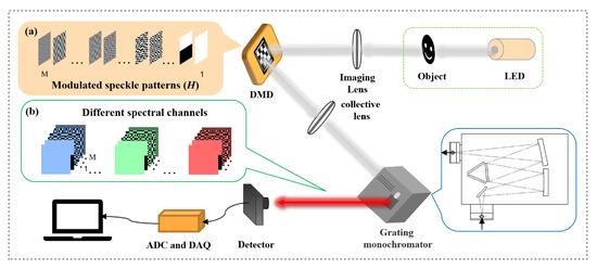
Figure 1.
Diagram of experimental setup. (a) The modulated matrices H. (b) The different spectral channels.
There is no doubt that DMD is one of the most-used core modulation devices in SPI because of its significant advantages of high modulation speed and wide wavelength ranges [56], whose optical unit is an array composed of hundreds of thousands of individually addressable optical micromirrors. Each micromirror can be individually oriented to , which represents 1 and 0 when a binary modulation is used. Usually, DMD is a binary optical intensity modulation device, while it can also realize the gray modulation at a low speed in some cases. In our experiments, i.e., in a typical SPI setup, a set of computer-generated binary patterns that are loaded onto the DMD are generally used to encode the optical intensity that is the target image imaged on the DMD. Commonly used modulation patterns include the random binary speckle patterns, the Hadamard transform patterns, and the Fourier transform patterns.
2.2. Data Collection and Processing
For simplicity and convenience, suppose the hyperspectral image is that is imaged by the imaging lens on the DMD, where is the spatial coordinate and is the wavelength. The Hadamard bases are chosen to encode the image of the target object, which would be mathematically expressed as [57]
where represents the encoded images that would be sent to the detection system. The spectrum detection system includes two parts of a grating monochromator to discretize the spectra of signals that is fed into it according to each central wavelength and an SPD that captures the bucket signals for each spectral band in turn. The kth () measurement process for the lth () spectral band can be described as
where L and M denotes the number of spectral bands and the number of modulation bases (or the sampling number). In SPI, and are used to reconstruct the images. In addition, if the size of the reconstruction image is pixels, the sampling rate () would be defined as .
In general, the bucket signals directly collected by SPD contain a lot of signal-related Poisson noise as well as noise caused by signal-independent environmental fluctuations, which will seriously affect the quality of the reconstruction image. Ferri et al. [58] proposed a differential GI (DGI) scheme in 2010 to overcome the influence of background noise, in which the relative value of object information was kept. It is shown that this scheme can greatly improve the SNR of reconstructed images. Inspired by the DGI, we proposed an iterative differential SPI scheme using a deep image prior-based network, where the detected bucket signals can be treated as [59]
Here, represents the intensity sum of the kth Hadamard basis , and the superscript t represents the iterative times of differential process.
2.3. Image Reconstruction by Untrained Neural Network
So far, we have established the process of data collection in single-pixel HSI. Now let us set up the process of reconstructing spectral data cubes using untrained neural networks.
In the field of SPI, object images are usually reconstructed using the correlation or CS algorithm. However, it is difficult for traditional methods to obtain high-quality reconstruction results at a low SR. The data-driven DL algorithm proved to be able to solve this challenging problem. Unfortunately, it is difficult to obtain sufficient training data in many tasks, and the limited generalization ability of the model, as well as the lengthy model training, are the big issues that needs to be addressed. Here, a single-pixel HSI reconstruction method based on an untrained neural network is proposed to make a compromise between the image quality and the computational cost. It integrates SPI’s physical model into a randomly initialized CNN to obtain high-quality reconstruction images by interacting with the imaging physics process during network optimization, which allows a low time-consumption in data preparation and image reconstruction [53]. The reconstruction process of the proposed method is shown in Figure 2a. Specifically, given a randomly initialized CNN (where is the deviation parameter of the network and z is the input image of the network), a function space is also defined (for each argument , there is a function in the function space corresponding to it). Assuming that the image we are looking for is in this space, we can get the image by looking for a reasonable . The output of the network is given by the following equation [48]
where z is the fuzzy reconstruction image obtained by CS. When the network output passes through the imaging model defined in Equation (2), a 1D bucket signal estimated by the network is obtained that is . It is worth noting that also uses the iterative differential instead of the original value, which is . The optimization process of the network can be defined as [50,59]
where is the total variation (TV) regularization constraint term. It is usually used to improve the quality of the reconstruction images. represents the mean square error between the measured bucket signals and the estimated ones by the network, which is also the loss of the network. What we need to do next is to choose a reasonable optimizer to update the weights and bias parameters of the network, as well as obtain the best reconstruction results, which is achieved by ending the network optimization early. Figure 2b shows the change of loss in the process from 1 to 1000 iteration steps of the network. The corresponding reconstruction images are shown in Figure 2c. One can clearly see that the reconstruction effect of the network is the best when the iteration is about 200 times.
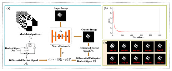
Figure 2.
Schematic diagram of network operation. (a) The reconstruction image process overview of the proposed method. The measured and can be used to obtain low-quality reconstruction results, which are then used as the input of the neural network. At the same time, the differential value of the is also input into the neural network. The output of the neural network is multiplied with to obtain the estimated bucket signals by the network. Then we obtain its differential value and measure the MSE between and as the loss function to optimize the weight of the neural network. (b) Loss value along with the iterative steps from 1 to 1000. (c) The corresponding reconstruction images of these steps (display every 100 times).
2.4. Network Architecture
In our method, a pure CNN of U-net [60] is used. The simplified structure of the neural network is shown in Figure 3. It consists of two main paths. The first is the encoder path (left side) which has the repeated application of two convolution blocks ( convolution (stride 1) + batch normalization + leaky ReLU) and a max pooling operation with stride 2 for downsampling. Second is the decoder path (right side) has an up-convolution block ( de-convolution (stride 2) + batch normalization + leaky ReLU) that halves the number of feature channels, and a concatenation with the corresponding feature map from the encoder path, and two convolution blocks. The network takes the degraded model of the object as its input, and outputs estimated high-quality reconstruction results. Sigmoid is used for the activation functions in the output layer. The loss function is the mean square error (MSE), and the Adam optimizer is adopted to optimize the weights and biases of the network with the default learning rate of 0.05 [50,60]. Note that the proposed algorithm was implemented in Python using a computer with an AMD CPU R5-5600H, 16 GB RAM. For an image of an object with a size of pixels, it is estimated that it only needs about 46 s to reconstruct a feasible result when is set to 12.5%.
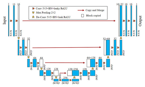
Figure 3.
Diagram of neural network architecture.
3. Results and Discussion
To demonstrate the effectiveness of our proposed method, a multispectral imaging experiment for a common third-order Rubik’s cube (with the RGB color distribution). Figure 4a is first demonstrated in the frameworks of SPI by removing the monochromator. The light source in Figure 1 was reset to be suitable for illuminating a reflecting object and an interference filter with a 10 nm bandwidth was inserted after, as shown in Figure 4b, where three interference filters with the central wavelengths of 440 nm, 532 nm, and 650 nm were selected, respectively, corresponding to the RGB channels. It should be noted that the number t of iterations of the differential bucket signals was chosen as 3, and the number of the network optimization (the standard of early stopping) was set as 200. For comparison, one of the well-used CS reconstruction algorithms in SPI was used, which is the famous total variation augmented Lagrangian alternating direction algorithm (TVAL3). Using three different colors of light, the images with the size of pixels are reconstructed by TVAL3 at the of 6.25%, 25%, and 50%, respectively, which are depicted in Figure 4c. For the proposed method based on the untrained neural network, the images in Figure 4d are recovered in the same conditions. It can be seen that our method can capture clearer images of the Rubik’s cube and distinguish more of its details under different spectral bands and different s. Especially the images reconstructed by TVAL3 have lost some features and details of the Rubik’s cube at the ultra-low of 6.25%, while those reconstructed by the untrained neural network-based method are still clear enough to recognize most details. Even when was increased to 50%, TVAL3 alone could not fully recover the details of the Rubik’s cube, such as the curved edge contour of each unit of the cube. More details are shown in Figure 4e, which are the enlargements of the images in the yellow dotted box of Figure 4c,d at the of 50%.
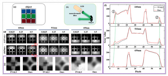
Figure 4.
Multispectral imaging of a third-order Rubik’s cube with RGB color distribution. The size of the reconstruction images is pixels. (a) The object. (b) A setting suitable for the reflecting object. (c,d) Reconstruction spectral images with central wavelengths of 440 nm, 532 nm, and 650 nm at the of 6.25%, 25%, and 50% by TVAL3 and the proposed method, respectively. (e) Enlargements of the images in the yellow dotted box of (c,d) at the of 50%. (f) The intensity profiles across the white dotted line in the reconstruction images at the of 50% in (c,d) vs. pixel number for different spectra bands. We select two groups of particular pixels ① and ②, which are connected across the spectral bands with the green dotted lines.
To further qualify the performance of our method, some comparisons between the details of the reconstruction images by two methods were made, where cross sections (see the white dotted line in Figure 4) of the reconstruction images at the of 50% in Figure 4c,d are examined and plotted in Figure 4f. In these cross-sections, two groups of particular pixels ① and ② are selected which correspond to the points with the maximum gray value in the region at the two upper and lower edges of the Rubik’s cube. In Figure 4f, two groups of particular pixels of the images that are reconstructed by the three colours of light are labelled and connected by the green dotted lines, respectively. It can be clearly seen that the white edge features of the Rubik’s cube in the images reconstructed by the proposed method can well be retained for all the three colours of light, while the upper edge features of the cube reconstructed by the TVAL3 in the 650 nm red light even almost completely disappear. Meanwhile, as the wavelength increases in Figure 4f, an obvious phenomenon appears that the corresponding pixel points in group ① move to the left (see the left green dotted line), which is because of the existence of longitudinal chromatism at the upper edge in the experiments. Fortunately, the very recently-proposed chromatic-aberration-corrected single-pixel HSI can solve this problem very well [61].
An unavoidable fact in the above experiments is that the reconstruction images by the red light are not as good as those at the other two wavelengths, because the red light has the weakest intensity. Considering this, a transmissive object of a USAF1951 resolution plate was selected as a target scene in the following single-pixel HSI experiments of Figure 1. The spectral range of imaging is set to 432–680 nm according to the spectrum range of light source and divided into 32 different bands with a step of about 8 nm. The size of the Hadamard basis is pixels and the rest of the parameters settings are the same as those in the above experiment. We first recovered target images of different spectral channels with an of 100% through the TVAL3, shown in Figure 5a. Overall, as expected, TVAL3 shows strong performance at an of 100%, achieving good results in the reconstruction of most spectral channels. However, TVAL3 faces significant challenges in reconstructing images at lower . At the same time, the proposed method shows excellent performance. The specific reconstruction results are shown in Figure 5 by comparison, where Figure 5b,c depict the target images of different spectral channels reconstructed by TVAL3 and the proposed method under different , respectively. A naked-eye evaluation shows that the quality of reconstruction images obtained by both methods decreases with the decrease of the . However, compared with TVAL3, the proposed method has a higher image quality and contrast. Specifically, the TVAL3 only obtains very vague reconstruction at an of 25%, with three vertical slits almost indistinguishable. In contrast, one can see that the proposed method obtains images with better vertical slit features as well as fewer artifacts under each spectral channel, which can be clearly seen from the background of the reconstruction images. In particular, TVAL3 fails at the of 12.5%, as evidenced by the inability to obtain detailed features of the object. By contrast, the proposed method is robust in most spectral channel image reconstruction and can reconstruct more of the details. It should be noted that the proposed method is based on untrained neural networks, so it does not require a large number of datasets and a large amount of time to train the neural networks.
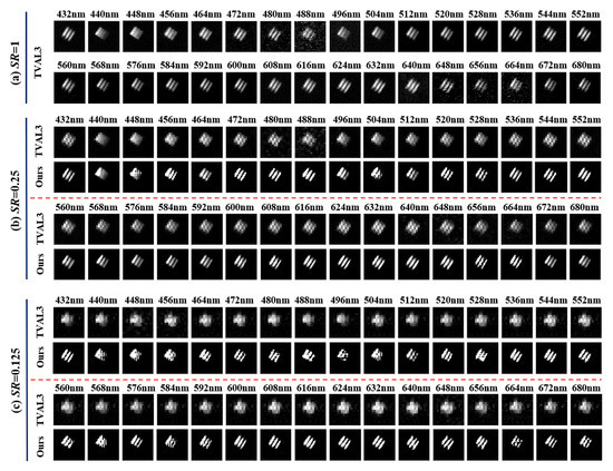
Figure 5.
The reconstructed 32 spectral bands hyperspectral images for a unit component of a USAF1951 resolution plate. Spectrum range is from 432 to 680 nm and the image size is pixels. The reconstruction images using TVAL3 at the of (a) 100% and the ones using TVAL3 and the proposed method at the of (b) 25% and (c) 12.5%, respectively.
More quantitative analysis results are shown in Figure 6. Two particular pixels are selected along the red dotted line (as shown in Figure 6a) for the reconstruction images obtained by the two methods at different and wavelengths, respectively. The pixel ① represents the light transmission part of the resolution plate (i.e., the intensity is 1), while the pixel ② represents the light, not transmission, part of the resolution plate, and its intensity is 0. Therefore, a simple way to measure the quality of the reconstruction image is to compare the difference between the intensity obtained by each method and the real at the two pixels. The specific comparison results are shown in Figure 6b (corresponding pixel ①) and Figure 6c (corresponding pixel ②), where the normalized intensity is used as a function of wavelength and . The black curve and the red one represent the results of TVAL3 at the of 12.5% and 25%, respectively. The blue curve and the green one represent the reconstruction results of the proposed method under the same conditions. It is not difficult to find that at the pixel ①, the value obtained by the proposed method at the ultra-low of 12.5% is better than that obtained by TVAL3 at any , which can be seen from the fact that the blue and green curves are above the other two curves. However, when the is 25%, the reconstruction results obtained by the proposed method at any wavelength are almost the same as the real ones. At the pixel ②, although the results obtained by the proposed method at some wavelengths are higher than those obtained by TVAL3 under the same conditions, the reconstruction results at other wavelengths are still closer to the real values, showing robust reconstruction performance.
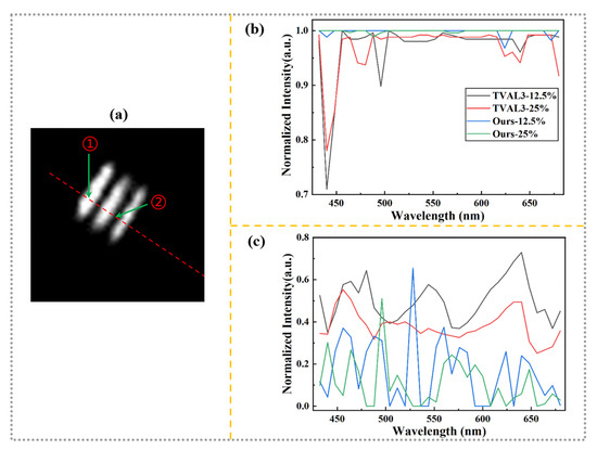
Figure 6.
Quantitative analysis results of the hyperspectral imaging. (a) Two particular pixels positions are selected along the red dotted line for the reconstruction images obtained by the two methods at different and wavelengths, respectively. (b,c) The results of the two methods obtained at different wavelengths and in the pixels ① and ②, respectively. The black, red, blue, and green curves represent the results of TVAL3 and the proposed method at the of 12.5% and 25%, respectively.
4. Conclusions
In conclusion, we have proposed and demonstrated a new single-pixel HSI scheme based on untrained CNN. Rather than using spectrometers or array detectors as usual, only a grating monochromator and an SPD are used for each spectral channel’s bucket detection. Such a setup allows it to have a lower cost, and wider spectral detection range though it is more time consuming. In the HSI experiments demonstrated, the proposed method is validated with an of 12.5% of the Nyquist sampling limit, and the image quality across a wide spectral range of 432–680 nm is much better than that by the commonly used TVAL3, which receives benefits from the strong denoising performance of the DIP-based untrained neural network and DGI. Therefore, our scheme can be used to reduce the amount of data needed to obtain high-quality images in microscopy, remote sensing, and satellite applications, as well as SPI applications.
In addition, it should be noted that although the untrained neural network method greatly saves the time previously used for network training, it still takes more time to obtain feasible results than the commonly used CS-based algorithm. Some feasible ways to improve the computational efficiency of this scheme include designing better neural network architecture, adopting better initialization strategy and learning rate, and the employment of a better computing platform. Another practical problem is that this method of combining specific imaging physical processes with an untrained neural network to obtain object reconstruction images requires accurate imaging models, which are extremely challenging tasks in some fields. Therefore, using this image reconstruction strategy in a complex environment will be a problem to be solved in the future. Last but not least, the proposed method only demonstrates the ability to reconstruct images of single spectral channels in each wavelength SPI, which actually is not the most time-efficient. In fact, several recent works [7,62] have reported more time-saving single-pixel HSI schemes, which allow reconstructing target images of multiple spectral channels from single data collected by the SPD. It is believed that the proposed method can perfectly fit these schemes, which benefits from an SPI’s accurate imaging physical model.
Author Contributions
Conceptualization, C.-H.W. and H.-Z.L.; methodology, C.-H.W.; validation, S.-H.B., R.-B.L. and X.-H.C.; writing—original draft preparation, C.-H.W.; writing—review and editing, X.-H.C.; data curation, C.-H.W. and H.-Z.L.; supervision, X.-H.C.; funding acquisition, X.-H.C. All authors have read and agreed to the published version of the manuscript.
Funding
The work was supported by the National Key Research and Development Program of China (Grant No. 2018YFB0504302).
Institutional Review Board Statement
Not applicable.
Data Availability Statement
Not applicable.
Conflicts of Interest
The authors declare no conflict of interest.
References
- Garini, Y.; Young, I.T.; McNamara, G. Spectral imaging: Principles and applications. Cytom. Part A J. Int. Soc. Anal. Cytol. 2006, 69, 735–747. [Google Scholar] [CrossRef] [PubMed]
- Govender, M.; Chetty, K.; Bulcock, H. A review of hyperspectral remote sensing and its application in vegetation and water resource studies. Water SA 2007, 33, 145–151. [Google Scholar] [CrossRef]
- Adam, E.; Mutanga, O.; Rugege, D. Multispectral and hyperspectral remote sensing for identification and mapping of wetland vegetation: A review. Wetl. Ecol. Manag. 2010, 18, 281–296. [Google Scholar] [CrossRef]
- Carrasco, O.; Gomez, R.B.; Chainani, A.; Roper, W.E. Hyperspectral imaging applied to medical diagnoses and food safety. In Proceedings of the Geo-Spatial and Temporal Image and Data Exploitation III, Orlando, FL, USA, 24 April 2003; SPIE: Bellingham, WA, USA, 2003; Volume 5097, pp. 215–221. [Google Scholar] [CrossRef]
- Afromowitz, M.A.; Callis, J.B.; Heimbach, D.M.; DeSoto, L.A.; Norton, M.K. Multispectral imaging of burn wounds: A new clinical instrument for evaluating burn depth. IEEE Trans. Biomed. Eng. 1988, 35, 842–850. [Google Scholar] [CrossRef] [PubMed]
- Lelieveld, J.; Evans, J.S.; Fnais, M.; Giannadaki, D.; Pozzer, A. The contribution of outdoor air pollution sources to premature mortality on a global scale. Nature 2015, 525, 367–371. [Google Scholar] [CrossRef]
- Bian, L.; Suo, J.; Situ, G.; Li, Z.; Fan, J.; Chen, F.; Dai, Q. Multispectral imaging using a single bucket detector. Sci. Rep. 2016, 6, 24752. [Google Scholar] [CrossRef]
- Donoho, D.L. Compressed sensing. IEEE Trans. Inf. Theory 2006, 52, 1289–1306. [Google Scholar] [CrossRef]
- Eldar, Y.C.; Kutyniok, G. Compressed Sensing: Theory and Applications; Cambridge University Press: Cambridge, UK, 2012. [Google Scholar]
- Arce, G.R.; Brady, D.J.; Carin, L.; Arguello, H.; Kittle, D.S. Compressive coded aperture spectral imaging: An introduction. IEEE Signal Process. Mag. 2013, 31, 105–115. [Google Scholar] [CrossRef]
- Lin, X.; Liu, Y.; Wu, J.; Dai, Q. Spatial-spectral encoded compressive hyperspectral imaging. ACM Trans. Graph. 2014, 33, 1–11. [Google Scholar] [CrossRef]
- Wagadarikar, A.; John, R.; Willett, R.; Brady, D. Single disperser design for coded aperture snapshot spectral imaging. Appl. Opt. 2008, 47, B44–B51. [Google Scholar] [CrossRef]
- Yuan, X.; Brady, D.J.; Katsaggelos, A.K. Snapshot compressive imaging: Theory, algorithms, and applications. IEEE Signal Process. Mag. 2021, 38, 65–88. [Google Scholar] [CrossRef]
- Lin, X.; Wetzstein, G.; Liu, Y.; Dai, Q. Dual-coded compressive hyperspectral imaging. Opt. Lett. 2014, 39, 2044–2047. [Google Scholar] [CrossRef]
- Garcia, H.; Correa, C.V.; Villarreal, O.; Pinilla, S.; Arguello, H. Multi-resolution reconstruction algorithm for compressive single pixel spectral imaging. In Proceedings of the 2017 25th European Signal Processing Conference (EUSIPCO), Kos Island, Greece, 28 August–2 September 2017; IEEE: Piscataway, NJ, USA, 2017; pp. 468–472. [Google Scholar] [CrossRef]
- Duarte, M.F.; Davenport, M.A.; Takhar, D.; Laska, J.N.; Sun, T.; Kelly, K.F.; Baraniuk, R.G. Single-pixel imaging via compressive sampling. IEEE Signal Process. Mag. 2008, 25, 83–91. [Google Scholar] [CrossRef]
- Shapiro, J.H. Computational ghost imaging. Phys. Rev. A 2008, 78, 061802. [Google Scholar] [CrossRef]
- Edgar, M.; Gibson, G.M.; Bowman, R.W.; Sun, B.; Radwell, N.; Mitchell, K.J.; Welsh, S.S.; Padgett, M.J. Simultaneous real-time visible and infrared video with single-pixel detectors. Sci. Rep. 2015, 5, 10669. [Google Scholar] [CrossRef]
- Schechner, Y.Y.; Nayar, S.K.; Belhumeur, P.N. Multiplexing for optimal lighting. IEEE Trans. Pattern Anal. Mach. Intell. 2007, 29, 1339–1354. [Google Scholar] [CrossRef]
- Morris, P.A.; Aspden, R.S.; Bell, J.E.; Boyd, R.W.; Padgett, M.J. Imaging with a small number of photons. Nat. Commun. 2015, 6, 5913. [Google Scholar] [CrossRef]
- Zhang, Z.; Ma, X.; Zhong, J. Single-pixel imaging by means of Fourier spectrum acquisition. Nat. Commun. 2015, 6, 6225. [Google Scholar] [CrossRef]
- Sun, B.; Edgar, M.P.; Bowman, R.; Vittert, L.E.; Welsh, S.; Bowman, A.; Padgett, M.J. 3D computational imaging with single-pixel detectors. Science 2013, 340, 844–847. [Google Scholar] [CrossRef]
- Tian, N.; Guo, Q.; Wang, A.; Xu, D.; Fu, L. Fluorescence ghost imaging with pseudothermal light. Opt. Lett. 2011, 36, 3302–3304. [Google Scholar] [CrossRef]
- Clemente, P.; Durán, V.; Torres-Company, V.; Tajahuerce, E.; Lancis, J. Optical encryption based on computational ghost imaging. Opt. Lett. 2010, 35, 2391–2393. [Google Scholar] [CrossRef] [PubMed]
- Zhao, C.; Gong, W.; Chen, M.; Li, E.; Wang, H.; Xu, W.; Han, S. Ghost imaging lidar via sparsity constraints. Appl. Phys. Lett. 2012, 101, 141123. [Google Scholar] [CrossRef]
- Magana-Loaiza, O.S.; Howland, G.A.; Malik, M.; Howell, J.C.; Boyd, R.W. Compressive object tracking using entangled photons. Appl. Phys. Lett. 2013, 102, 231104. [Google Scholar] [CrossRef]
- Li, C.; Sun, T.; Kelly, K.F.; Zhang, Y. A compressive sensing and unmixing scheme for hyperspectral data processing. IEEE Trans. Image Process. 2011, 21, 1200–1210. [Google Scholar] [CrossRef]
- Magalhães, F.; Araújo, F.M.; Correia, M.; Abolbashari, M.; Farahi, F. High-resolution hyperspectral single-pixel imaging system based on compressive sensing. Opt. Eng. 2012, 51, 071406. [Google Scholar] [CrossRef]
- Welsh, S.S.; Edgar, M.P.; Bowman, R.; Jonathan, P.; Sun, B.; Padgett, M.J. Fast full-color computational imaging with single-pixel detectors. Opt. Express 2013, 21, 23068–23074. [Google Scholar] [CrossRef]
- Radwell, N.; Mitchell, K.J.; Gibson, G.M.; Edgar, M.P.; Bowman, R.; Padgett, M.J. Single-pixel infrared and visible microscope. Optica 2014, 1, 285–289. [Google Scholar] [CrossRef]
- August, Y.; Vachman, C.; Rivenson, Y.; Stern, A. Compressive hyperspectral imaging by random separable projections in both the spatial and the spectral domains. Appl. Opt. 2013, 52, D46–D54. [Google Scholar] [CrossRef]
- Hahn, J.; Debes, C.; Leigsnering, M.; Zoubir, A.M. Compressive sensing and adaptive direct sampling in hyperspectral imaging. Digit. Signal Process. 2014, 26, 113–126. [Google Scholar] [CrossRef]
- Tao, C.; Zhu, H.; Wang, X.; Zheng, S.; Xie, Q.; Wang, C.; Wu, R.; Zheng, Z. Compressive single-pixel hyperspectral imaging using RGB sensors. Opt. Express 2021, 29, 11207–11220. [Google Scholar] [CrossRef]
- Yi, Q.; Heng, L.Z.; Liang, L.; Guangcan, Z.; Siong, C.F.; Guangya, Z. Hadamard transform-based hyperspectral imaging using a single-pixel detector. Opt. Express 2020, 28, 16126–16139. [Google Scholar] [CrossRef]
- Jin, S.; Hui, W.; Wang, Y.; Huang, K.; Shi, Q.; Ying, C.; Liu, D.; Ye, Q.; Zhou, W.; Tian, J. Hyperspectral imaging using the single-pixel Fourier transform technique. Sci. Rep. 2017, 7, 45209. [Google Scholar] [CrossRef]
- Zhang, Z.; Liu, S.; Peng, J.; Yao, M.; Zheng, G.; Zhong, J. Simultaneous spatial, spectral, and 3D compressive imaging via efficient Fourier single-pixel measurements. Optica 2018, 5, 315–319. [Google Scholar] [CrossRef]
- Moshtaghpour, A.; Bioucas-Dias, J.M.; Jacques, L. Compressive hyperspectral imaging: Fourier transform interferometry meets single pixel camera. arXiv 2018, arXiv:1809.00950. [Google Scholar] [CrossRef]
- LeCun, Y.; Bengio, Y.; Hinton, G. Deep learning. Nature 2015, 521, 436–444. [Google Scholar] [CrossRef]
- Arias, F.; Sierra, H.; Arzuaga, E. A Framework For An Artificial Neural Network Enabled Single Pixel Hyperspectral Imager. In Proceedings of the 2019 10th Workshop on Hyperspectral Imaging and Signal Processing: Evolution in Remote Sensing (WHISPERS), Amsterdam, The Netherlands, 24–26 September 2019; pp. 1–5. [Google Scholar] [CrossRef]
- Xiong, Z.; Shi, Z.; Li, H.; Wang, L.; Liu, D.; Wu, F. HSCNN: CNN-Based Hyperspectral Image Recovery From Spectrally Undersampled Projections. In Proceedings of the IEEE International Conference on Computer Vision (ICCV) Workshops, Venice, Italy, 22–29 October 2017. [Google Scholar]
- Barbastathis, G.; Ozcan, A.; Situ, G. On the use of deep learning for computational imaging. Optica 2019, 6, 921–943. [Google Scholar] [CrossRef]
- Lyu, M.; Wang, W.; Wang, H.; Wang, H.; Li, G.; Chen, N.; Situ, G. Deep-learning-based ghost imaging. Sci. Rep. 2017, 7, 17865. [Google Scholar] [CrossRef]
- He, Y.; Wang, G.; Dong, G.; Zhu, S.; Chen, H.; Zhang, A.; Xu, Z. Ghost imaging based on deep learning. Sci. Rep. 2018, 8, 6469. [Google Scholar] [CrossRef]
- Higham, C.F.; Murray-Smith, R.; Padgett, M.J.; Edgar, M.P. Deep learning for real-time single-pixel video. Sci. Rep. 2018, 8, 2369. [Google Scholar] [CrossRef]
- Wang, F.; Wang, H.; Wang, H.; Li, G.; Situ, G. Learning from simulation: An end-to-end deep-learning approach for computational ghost imaging. Opt. Express 2019, 27, 25560–25572. [Google Scholar] [CrossRef]
- Shang, R.; Hoffer-Hawlik, K.; Wang, F.; Situ, G.; Luke, G.P. Two-step training deep learning framework for computational imaging without physics priors. Opt. Express 2021, 29, 15239–15254. [Google Scholar] [CrossRef] [PubMed]
- Jin, K.H.; McCann, M.T.; Froustey, E.; Unser, M. Deep convolutional neural network for inverse problems in imaging. IEEE Trans. Image Process. 2017, 26, 4509–4522. [Google Scholar] [CrossRef] [PubMed]
- Ulyanov, D.; Vedaldi, A.; Lempitsky, V. Deep image prior. In Proceedings of the IEEE Conference on Computer Vision and Pattern Recognition (CVPR), Salt Lake City, UT, USA, 18–23 June 2018; pp. 9446–9454. [Google Scholar]
- Wang, F.; Bian, Y.; Wang, H.; Lyu, M.; Pedrini, G.; Osten, W.; Barbastathis, G.; Situ, G. Phase imaging with an untrained neural network. Light Sci. Appl. 2020, 9, 77. [Google Scholar] [CrossRef] [PubMed]
- Wang, F.; Wang, C.; Chen, M.; Gong, W.; Zhang, Y.; Han, S.; Situ, G. Far-field super-resolution ghost imaging with a deep neural network constraint. Light Sci. Appl. 2022, 11, 1–11. [Google Scholar] [CrossRef] [PubMed]
- Wang, F.; Wang, C.; Deng, C.; Han, S.; Situ, G. Single-pixel imaging using physics enhanced deep learning. Photonics Res. 2022, 10, 104–110. [Google Scholar] [CrossRef]
- Meng, Z.; Yu, Z.; Xu, K.; Yuan, X. Self-Supervised Neural Networks for Spectral Snapshot Compressive Imaging. In Proceedings of the IEEE/CVF International Conference on Computer Vision (ICCV), Montreal, BC, Canada, 11–17 October 2021; pp. 2622–2631. [Google Scholar]
- Lin, S.; Wang, X.; Zhu, A.; Xue, J.; Xu, B. Steganographic optical image encryption based on single-pixel imaging and an untrained neural network. Opt. Express 2022, 30, 36144–36154. [Google Scholar] [CrossRef]
- Lin, J.; Yan, Q.; Lu, S.; Zheng, Y.; Sun, S.; Wei, Z. A Compressed Reconstruction Network Combining Deep Image Prior and Autoencoding Priors for Single-Pixel Imaging. Photonics 2022, 9, 343. [Google Scholar] [CrossRef]
- Li, M.; Yan, L.; Yang, R.; Liu, Y. Fast single-pixel imaging based on optimized reordering Hadamard basis. Acta Phys. Sin. 2019, 68, 064202. [Google Scholar] [CrossRef]
- Gibson, G.M.; Johnson, S.D.; Padgett, M.J. Single-pixel imaging 12 years on: A review. Opt. Express 2020, 28, 28190–28208. [Google Scholar] [CrossRef]
- Yang, S.; Qin, H.; Yan, X.; Yuan, S.; Yang, T. Deep spatial-spectral prior with an adaptive dual attention network for single-pixel hyperspectral reconstruction. Opt. Express 2022, 30, 29621–29638. [Google Scholar] [CrossRef]
- Ferri, F.; Magatti, D.; Lugiato, L.A.; Gatti, A. Differential Ghost Imaging. Phys. Rev. Lett. 2010, 104, 253603. [Google Scholar] [CrossRef]
- Wang, C.H.; Bie, S.H.; Lv, R.B.; Li, H.Z.; Fu, Q.; Bao, Q.Q.; Meng, S.Y.; Chen, X.H. High-quality single-pixel imaging in a diffraction-limited system using a deep image prior-based network. Opt. Express, 2022; submitted. [Google Scholar]
- Ronneberger, O.; Fischer, P.; Brox, T. U-Net: Convolutional Networks for Biomedical Image Segmentation. In Proceedings of the Medical Image Computing and Computer-Assisted Intervention—MICCAI 2015, Munich, Germany, 5–9 October 2015; Springer International Publishing: Cham, Switzerland, 2015; Volume 9351, pp. 234–241. [Google Scholar] [CrossRef]
- Liu, Y.; Yang, Z.H.; Yu, Y.J.; Wu, L.A.; Song, M.Y.; Zhao, Z.H. Chromatic-Aberration-Corrected Hyperspectral Single-Pixel Imaging. Photonics 2023, 10, 7. [Google Scholar] [CrossRef]
- Li, Z.; Suo, J.; Hu, X.; Deng, C.; Fan, J.; Dai, Q. Efficient single-pixel multispectral imaging via non-mechanical spatio-spectral modulation. Sci. Rep. 2017, 7, 41435. [Google Scholar] [CrossRef]
Disclaimer/Publisher’s Note: The statements, opinions and data contained in all publications are solely those of the individual author(s) and contributor(s) and not of MDPI and/or the editor(s). MDPI and/or the editor(s) disclaim responsibility for any injury to people or property resulting from any ideas, methods, instructions or products referred to in the content. |
© 2023 by the authors. Licensee MDPI, Basel, Switzerland. This article is an open access article distributed under the terms and conditions of the Creative Commons Attribution (CC BY) license (https://creativecommons.org/licenses/by/4.0/).