A Hybrid Deep Reinforcement Learning Architecture for Optimizing Concrete Mix Design Through Precision Strength Prediction

Abstract

Concrete mix design plays a pivotal role in ensuring the mechanical performance, durability, and sustainability of construction projects. However, the nonlinear interactions among the mix components challenge traditional approaches in predicting compressive strength and optimizing proportions. This study presents a two-stage hybrid framework that integrates deep learning with reinforcement learning to overcome these limitations. First, a Convolutional Neural Network–Long Short-Term Memory (CNN–LSTM) model was developed to capture spatial–temporal patterns from a dataset of 1030 historical concrete samples. The extracted features were enhanced using an eXtreme Gradient Boosting (XGBoost) meta-model to improve generalizability and noise resistance. Then, a Dueling Double Deep Q-Network (Dueling DDQN) agent was used to iteratively identify optimal mix ratios that maximize the predicted compressive strength. The proposed framework outperformed ten benchmark models, achieving an MAE of 2.97, RMSE of 4.08, and R² of 0.94. Feature attribution methods—including SHapley Additive exPlanations (SHAP), Elasticity-Based Feature Importance (EFI), and Permutation Feature Importance (PFI)—highlighted the dominant influence of cement content and curing age, as well as revealing non-intuitive effects such as the compensatory role of superplasticizers in low-water mixtures. These findings demonstrate the potential of the proposed approach to support intelligent concrete mix design and real-time optimization in smart construction environments.

1. Introduction

In recent decades, the construction industry has faced increasing pressure to enhance quality, extend structural durability, and reduce operational costs [1]. With the rapid expansion of urbanization, the development of critical infrastructure, and the demand for resilient civil projects under harsh environmental conditions, engineers have become increasingly focused on optimizing materials and execution processes [2]. Among the various construction materials, concrete stands out as the most widely used and plays a fundamental role in ensuring structural stability and safety. Despite its long-standing usage, selecting an optimal mix design for concrete remains a complex and multi-objective problem, as its mechanical properties and long-term performance are highly sensitive to the proportion of its constituents, including cement, water, aggregates, and chemical admixtures [3]. Scientifically designing these proportions to simultaneously meet engineering, economic, and environmental constraints has thus become one of the core challenges in civil engineering and materials science [4].

In response to the complexities of concrete mix design, numerous studies have sought to model the relationships between constituent materials and the mechanical properties of concrete in a more data-driven and systematic manner [5]. Over the past two decades, statistical methods, machine learning algorithms, and optimization techniques have been widely employed to improve the accuracy of compressive strength prediction based on experimental datasets [6]. While these approaches have contributed valuable insights, most existing research has primarily focused on the prediction task, without extending into intelligent decision-making for selecting optimal mix designs under dynamic or real-world constraints [7,8]. Moreover, many of the current models exhibit sensitivity to data uncertainty and environmental variability, lacking mechanisms for noise robustness, performance stability, and adaptability to operational conditions.

One of the fundamental challenges in concrete mix design lies in simultaneously achieving accurate strength prediction and optimal decision-making under uncertainty, environmental variability, and practical constraints [9]. Addressing this issue requires the development of models that not only capture the complex nonlinear relationships between input constituents and mechanical performance but also adaptively respond to dynamic and uncertain scenarios. Despite notable advancements in machine learning and the proliferation of predictive modeling approaches, most existing studies fall short in integrating predictive accuracy with robust decision-making capabilities [10]. This gap underscores the urgent need for innovative and adaptive frameworks that can leverage hybrid algorithms to deliver intelligent, resilient, and practically applicable solutions for optimizing concrete mix compositions.

To address the challenge of accurately modeling the relationship between concrete mix composition and compressive strength, this study proposes a hybrid predictive framework that leverages the complementary strengths of deep learning and ensemble methods. Specifically, a hybrid neural architecture combining a Convolutional Neural Network (CNN) and a Long Short-Term Memory (LSTM) network—collectively referred to as CNN-LSTM—is employed to extract both spatial and temporal patterns from the data. In the first phase, a dataset comprising 1030 concrete mix samples was obtained from a publicly available Kaggle repository. After a rigorous preprocessing pipeline—including feature normalization, correlation-based variable selection, and time series structuring via a sliding window technique—the CNN-LSTM model was developed to capture multidimensional dependencies within the data. The intermediate feature representations extracted by the CNN-LSTM were then used as input to an eXtreme Gradient Boosting (XGBoost) model acting as a meta-learner. This two-stage architecture enabled the integration of deep hierarchical feature extraction with the generalization power of gradient boosting, resulting in a more accurate, stable, and noise-resilient prediction of compressive strength compared to conventional single-model approaches.

In the second phase, this study addresses the gap in robust and adaptive decision-making by developing a reinforcement learning (RL) framework based on the Dueling Double Deep Q-Network (Dueling DDQN) algorithm. The learning agent was designed to autonomously select the most suitable concrete mix under varying construction scenarios, using the predictive outcomes from Phase I as the simulated environment. The state space included normalized project features, while the action space consisted of four predefined concrete mix types. The reward function was carefully constructed to jointly encourage high compressive strength, output stability, and cost-efficiency. To evaluate the reliability of the proposed decision-making framework, a noise sensitivity analysis was conducted by injecting Gaussian perturbations at multiple levels. The results demonstrated that the hybrid agent outperformed baseline models in maintaining stable performance under uncertainty, making it a suitable tool for practical applications such as smart construction, adaptive quality control, and resilient material design.

This study leverages two core methodological approaches: RL and hybrid neural network architecture. RL is a branch of machine learning in which an autonomous agent learns to make optimal decisions through iterative interactions with an environment and by receiving feedback in the form of rewards [11]. RL is particularly well-suited for sequential decision-making problems and dynamic environments characterized by uncertainty, where traditional rule-based or static models often fall short [12]. In parallel, the hybrid neural network architecture employed in this study integrates CNNs and Long Short-Term Memory (LSTM) networks. CNNs are effective in extracting spatial or local patterns from structured input data, while LSTMs are designed to capture long-term temporal dependencies in sequential data [13,14]. The fusion of these two architectures enables the model to jointly understand both spatial correlations and temporal dynamics inherent in concrete mix data. This dual-framework provides the foundation for a system that not only performs accurate predictions but also adapts intelligently to evolving real-world conditions.

In light of the identified gaps in the literature and the need for frameworks that can simultaneously support accurate prediction and robust decision-making, the primary objective of this study is to develop a data-driven, intelligent, and adaptive model for concrete mix design under uncertainty. To this end, the research aims to construct a hybrid architecture capable of extracting spatial and temporal patterns from concrete composition data to enable precise prediction of compressive strength, while also utilizing these predictions within a RL –based decision support system. The proposed model is expected to deliver not only high predictive accuracy but also the ability to select optimal mix designs with respect to performance stability, efficiency, and cost-effectiveness in real-world, noisy environments. The central contribution lies in integrating these two components—prediction and decision optimization—into a unified, deployable framework for practical applications in construction materials engineering.

To achieve the aforementioned objectives, the structure of this study is organized into six main sections. In Section 2, we review the relevant literature on concrete mix design, predictive modeling, and decision-making under uncertainty. Section 3 outlines the proposed methodology, including the hybrid deep learning framework and the RL-based optimization model. Section 4 presents the experimental results and performance evaluation of the proposed system. In Section 5, we provide a detailed discussion of the findings, implications, and limitations. Finally, Section 6 concludes the study by summarizing the key contributions and suggesting directions for future research.

2. Literature Review

This section reviews prior research in two key areas relevant to this study. Section 2.1 examines methods for predicting concrete compressive strength, ranging from traditional models to advanced machine and deep learning approaches. Section 2.2 explores how RL has been applied to optimize concrete mix design and similar material composition problems. Finally, Section 2.3 identifies the research gaps in the existing literature and highlights the contributions of the present study.

2.1. Prediction of Concrete Compressive Strength

Predicting the compressive strength of concrete has long been a central topic in civil engineering and construction materials research, as it directly impacts the safety, durability, and performance of structures. Over the past several decades, a variety of modeling techniques have been developed to estimate this mechanical property. Initially, empirical formulas and regression-based models grounded in engineering expertise were dominant. However, as datasets expanded and the complexity of inter-variable relationships increased, machine learning (ML) and deep learning (DL) approaches emerged as more powerful and accurate alternatives [15]. These data-driven techniques are capable of capturing complex nonlinear dependencies among variables such as the water-to-cement ratio, admixture content, and curing age. This subsection reviews the evolution of these predictive models and critically examines their strengths and limitations in accurately estimating concrete compressive strength.

Among the recent advancements in this domain, several studies have proposed innovative modeling techniques to improve prediction accuracy, especially under constraints such as limited data availability, material heterogeneity, and the need for model interpretability. Zhang, Yuan [16] tackled the challenge of data scarcity in deep learning-based concrete strength prediction by proposing a hybrid method named Decision Tree-guided Artificial Neural Network Pretraining (TANNP). Their model effectively leveraged the decision tree’s robustness on small datasets to guide the pretraining of a neural network, significantly improving predictive accuracy. By reducing the RMSE from 5.10 to 3.26 MPa and raising R² from 0.91 to 0.97, they demonstrated that strategic pretraining can overcome limitations of data-hungry models. Building on this direction, Miao et al. [17] focused on the eco-friendly design of recycled aggregate self-compacting concrete (RA-SCC) by evaluating five interpretable machine learning algorithms. Among them, XGBoost outperformed others (R² = 0.909), and SHapley Additive exPlanations (SHAP) analysis revealed the nuanced influence of variables, with cement and age contributing positively, while recycled materials had negative impacts. This interpretability deepened insights into sustainable mix behavior. Expanding the predictive frontier to geopolymer concrete, Khosravi and Bahram [18] developed an Artificial Neural Network (ANN)-based hybrid framework integrated with Genetic Algorithm, Particle Swarm Optimization, and Levenberg–Marquardt algorithm. They showed that ANN-LM achieved the highest accuracy, emphasizing the importance of chemical variability in fly ash and activators. Their study also underlined the role of AI in optimizing green concrete designs. Collectively, these works reveal a trend toward hybrid and interpretable models tailored to both conventional and sustainable concrete, while addressing key limitations such as data scarcity, material heterogeneity, and model transparency.

Building upon the growing interest in hybrid deep learning models, Liu, Yu [19] proposed a CNN-BiLSTM-MA framework that synergizes convolutional feature extraction, bidirectional temporal learning, and multi-head attention for predicting the compressive strength of concrete at different curing ages. Their model, trained on eight input variables and benchmarked against five classical machine learning baselines (e.g., XGBoost, LightGBM), achieved superior performance (RMSE = 1.21, MAE = 0.85), highlighting the efficacy of attention-based architectures in capturing complex interdependencies. Zhao, Zhang [20], on the other hand, addressed the prediction of compressive strength for multiple types of fiber-reinforced concrete (FRC), a topic often overlooked in prior research. They introduced a hybrid meta-modeling approach combining DNN, GRNN, and XGBoost optimized through PSO, BO, and BES. The BES-XGBoost model yielded the most accurate results, and SHAP analysis further illuminated the nonlinear influence of fiber types on strength behavior. In contrast to purely data-driven approaches, Sathurshan, Derakhshan [21] adopted an experimental and analytical methodology to evaluate compressive strength in grouted and un-grouted dry-stack concrete block masonry. By testing 80 wall specimens with varied grout and block types, they reported strength increases up to 152% in grouted configurations and examined the predictive validity of standard formulae. While not machine learning-based, their contribution offers critical empirical insight that can inform and validate future data-driven models. Collectively, these studies not only expand the spectrum of concrete types analyzed but also demonstrate the rising prominence of hybridized, interpretable, and experimentally grounded approaches in compressive strength prediction research.

In recent studies, sustainability-oriented modeling has gained momentum by integrating recycled and alternative materials into concrete mix design while leveraging advanced machine learning. Farouk, ElGazzar [22] explored the prediction of compressive strength in treated wastewater concrete (TWWC) using five tree-based algorithms and a stacking ensemble, trained on 499 observations synthesized from 45 global studies. Their XGBoost-based model, enhanced through Optuna hyperparameter tuning and validated via laboratory experiments, achieved strong generalizability (R² = 0.949; test RMSE = 3.57 MPa), while SHAP analysis revealed that sulfate content and total dissolved solids were the most influential predictors. Similarly, Sinkhonde, Bezabih [23] employed ensemble ML methods to estimate the strength of concrete incorporating waste tire rubber (WTR) and clay brick powder (CBP). Among ANN, RF, SVM, and DT models, SVM exhibited the best performance. SHAP analysis indicated WTR as the most critical factor in strength variation, confirming the feasibility of ML in managing complex waste-inclusive mixes. Complementing these works, Philip and Marakkath [24] focused on GGBS-based geopolymer concrete and conducted a comparative optimization of XGBoost hyperparameters using PSO, ESOA, GWO, and WOA. Their PSO-optimized model achieved high accuracy (R² = 0.974; RMSE = 2.715), and SHAP interpretation highlighted the importance of GGBS content, curing age, and sodium hydroxide molarity. Their inclusion of a GUI for practical deployment underscores the growing emphasis on real-world applicability. Collectively, these studies not only reflect the evolving environmental priorities in concrete technology but also underline the role of interpretable, ensemble-based, and optimization-driven ML approaches in enabling robust prediction under material variability and uncertainty.

Building upon the growing trend of leveraging artificial intelligence for enhanced prediction accuracy, Amar [25] conducted a large-scale comparative study involving over 5000 concrete mix designs incorporating supplementary cementitious materials (SCMs). The study evaluated several models, including ANN, SVM, RF, and gradient-boosted trees (GBT), and found GBT to be the most accurate based on R², RMSE, and MAPE. This work reaffirmed the value of ensemble and deep models in generalizing across diverse concrete formulations. Similarly, Lu, Zhou [26] explored the prediction of compressive strength in basalt fiber-reinforced rubberized concrete (BFRRC), where traditional models struggled due to nonlinearity introduced by dual-modification with rubber particles and basalt fibers. To address this, they trained an ANN on 254 experimental cases and derived an explicit predictive equation based on five critical inputs. This not only improved forecasting accuracy but also enabled practical application in low-carbon design strategies. Complementing these studies, Yu, Wang [27] introduced a hybrid intelligent model combining Gaussian Process Regression with Improved Whale Optimization Algorithm (IWOA-GPR) to predict the strength of silica fume-enhanced self-compacting concrete (SCC). Their model outperformed baseline learners such as SVM and RF, achieving R² = 0.95 and an RMSE of 6.52 on the test set.

Expanding the frontier of concrete strength prediction, Anwar, Qurashi [28] conducted a rigorous comparative analysis of multiple ML models to forecast the 28-day compressive strength of fly ash-based geopolymer concrete (FAGP). By assembling 563 samples from 55 publications, the study benchmarked models including ANN, Support Vector Machine (SVM), K-Nearest Neighbors (KNN), and ensemble-based decision trees. The results revealed that ANN and boosting techniques significantly outperformed others, achieving R² values above 0.90 and demonstrating the practical utility of ensemble learning in capturing complex nonlinear dependencies inherent in geopolymer systems. SHAP analysis confirmed fly ash content and curing temperature as critical predictive variables, reinforcing their role in optimizing mix design. Complementing this, Dahish and Almutairi [29] investigated strength prediction in nano-modified concrete under elevated temperatures using RF and M5P models. Their analysis focused on mixes containing nano-alumina and carbon nanotubes (CNTs), revealing that RF achieved superior performance (R² = 0.9921, MAPE = 1.72%) across all temperature ranges. Sensitivity and SHAP analyses underscored temperature as the dominant factor, while optimal nano-admixture ratios were identified for various heat exposures. Collectively, these studies underscore the growing precision and generalizability of machine learning frameworks in modeling complex concrete systems, spanning traditional, geopolymer, and nano-enhanced formulations under diverse environmental scenarios.

2.2. Reinforcement Learning for Concrete Mix Optimization

In recent years, RL has emerged as a powerful paradigm for sequential decision-making problems across various engineering domains. Within the context of concrete mix design, RL offers a promising avenue to not only optimize material combinations but also adaptively learn from iterative feedback to improve long-term performance objectives. Unlike traditional optimization or supervised learning approaches that require static datasets, RL frameworks enable the agent to interact with an environment—representing the material property landscape—and discover optimal policies for mix adjustment based on reward signals such as compressive strength, cost-efficiency, or sustainability. This subsection reviews the integration of RL techniques into civil engineering applications, with a particular focus on how these models are employed to optimize concrete composition and performance under uncertain or complex design spaces.

Building upon the promise of RL in structural material design, recent studies have showcased its effectiveness across diverse concrete-related optimization challenges. Ma, Wang and Chen [30] addressed the safety-critical problem of bond strength prediction in 3D-printed reinforced concrete by leveraging a trustworthy machine learning framework based on Natural Gradient Boosting. Their approach incorporated probabilistic estimation to quantify predictive uncertainty, achieving a 94.5% safety rate and outperforming conventional deterministic models, thus aiding in the design of reinforcement embedment length. In a more dynamic design context, Lin, Fu [31] introduced a deep RL framework using Proximal Policy Optimization (PPO) for the automated design of steel–concrete composite beams. Their agent, modeled via a Markov Decision Process and trained on real engineering scenarios, demonstrated superior cost-efficiency and compliance with structural standards when benchmarked against Differential Evolution. Further extending the scope of RL to production scheduling, Du and Li [32] developed a distributed precast concrete scheduling algorithm based on coordinated Double Deep Q-Networks (DDQNs). By integrating local, global, and selection DQNs, the system adaptively minimized tardiness penalties and electricity costs in multi-factory environments. Collectively, these works underline the versatility of RL, from structural reliability to cost-aware production planning, and set the foundation for its application in optimizing concrete mix design.

Further advancements in concrete-related design and operations have embraced RL to optimize both logistical and structural challenges in the built environment. Chen, Wang [33] proposed a model-based RL method to optimize the scheduling of electric ready-mixed concrete (ERM) vehicles, a task complicated by time-dependent electricity pricing and operational constraints unique to electric fleets. By formulating the task as a Markov Decision Process (MDP) and introducing a novel algorithm—Parallel-Masked-Decaying Monte Carlo Tree Search (PMD-MCTS)—they successfully reduced operational delays and computational cost, demonstrating its superiority over baseline methods in a real-world case study. Complementing this logistical focus, Liu, Qi [34] addressed the geometric and structural complexity of precast concrete wall panels. Their innovative framework combined Generative Adversarial Networks (GANs) with Deep Reinforcement Learning (DRL) to resolve rebar clashes during automated design. By learning from existing 2D rebar drawings and adhering to buildability constraints, their method reduced engineering time by 80%, showing that DRL can handle intricate spatial design constraints in civil structures. Jayasinghe, Wei Chen [35] applied a pure machine learning (ML) approach—without RL—to predict the shear strength of recycled aggregate concrete (RAC) beams. Using a dataset of 401 beams and eight ML algorithms, they identified XGBoost as the best performer, validated through SHAP-based interpretability and code-based comparisons.

The exploration of RL in concrete-related applications continues to expand into domains of scheduling, structural reinforcement, and material durability. Kim, Kim [36] focused on the scheduling of precast concrete production, a domain traditionally dominated by dispatching rules and metaheuristics. By implementing a RL-based model, they achieved significant improvements in scheduling efficiency, reducing total tardiness by up to 12% while maintaining real-time responsiveness. In parallel, Liu, Liu [37] tackled the challenge of rebar clashes in reinforced concrete frame structures by developing a multi-agent system where each rebar acts as an intelligent agent. Using Q-learning integrated with BIM, their framework dynamically planned rebar paths while adhering to constructability and design constraints, outperforming existing rule-based systems. Luan, Fan [38], diverging from RL, investigated corrosion characteristics in concrete, developing a predictive model for critical corrosion depth through analytical methods. While not data-driven, their work complements learning-based approaches by offering mechanistic insights into long-term durability under electrochemical degradation. Lastly, Wan, Xu [39] returned to RL to optimize the internal vascular configuration in self-healing concrete. By interacting with a physics-based simulation environment, their agent learned to configure vascular structures to maximize fracture energy, demonstrating RL’s capability for geometry-aware material design. Collectively, these studies illustrate how RL can augment traditional engineering knowledge—from optimizing complex construction schedules and preventing rebar clashes to innovating smart material design—while also showing that physics-based analytical models still provide essential foundational insights in contexts less suited to learning algorithms.

2.3. Research Gap and Contribution

A comprehensive review of existing studies (as summarized in

Table 1. Summary of Previous Studies.

Reference	Research Objective	Algorithms Used	HM	RL	ML/DL
					DL	ML
Zhang, Yuan [16]	Predict compressive strength using treated wastewater	DTR, RFR, ETR, GTB, XGB, Stacking Ensemble	✔️			✔️
Miao, Gao [17]	Predict strength of concrete with waste tire rubber and brick powder	ANN, RF, DT, SVM			✔️	✔️
Khosravi and Bahram [18]	Predict strength of GGBS-based geopolymer concrete with optimized metaheuristics	XGBoost + PSO, ESOA, GWO, WOA	✔️			✔️
Liu, Yu [19]	Compare different AI methods for predicting compressive strength	ANN, DL, GLM, DT, RF, SVM, GBT			✔️	✔️
Zhao, Zhang [20]	Predict compressive strength of basalt fiber reinforced rubberized concrete	ANN			✔️
Sathurshan, Derakhshan [21]	Predict SCC strength with silica fume using IWOA-GPR model	GPR + IWOA	✔️			✔️
Farouk, ElGazzar [22]	Compare ML models for predicting strength of fly ash-based concrete	MLR, ANN, SVM, KNN, DT	✔️		✔️	✔️
Sinkhonde, Bezabih [23]	Predict strength of nano-material concrete under high temperature	RF, M5P, LR				✔️
Lin, Fu [31]	Automated design of steel-concrete composite beams using DRL.	PPO, DE	✔️	✔️
Liu, Qi [34]	Clash-free rebar design in precast panels using GAN and DRL integrated with BIM.	GAN, DRL	✔️	✔️	✔️
Jayasinghe, Wei Chen [35]	Shear strength prediction of RAC beams using machine learning algorithms.	LR, KNN, RF, AdaBoost, GB, XGBoost, CatBoost, LightGBM				✔️
Kim, Kim [36]	Scheduling of precast concrete production using RL for fast real-time optimization.	unspecified variant		✔️
Liu, Liu [37]	Clash resolution in concrete frames using Q-learning and BIM for automatic rebar path planning.	Q-learning	✔️	✔️
Luan, Fan [38]	Modeling corrosion depth at concrete cover cracking in accelerated environments.	Statistical modeling
Wan, Xu [39]	Optimizing vascular configurations in self-healing concrete using RL with Abaqus simulation.	RL (custom with simulation)	✔️	✔️
This study	Strength prediction and mix optimization of concrete using a hybrid deep and RL model	CNN, LSTM, XGBoost, Dueling DDQN	✔️	✔️	✔️	✔️

Note: Reinforcement Learning (RL), Hybrid Model (HM), Proximal Policy Optimization (PPO), Differential Evolution (DE), Natural Gradient Boosting (NGB).

) reveals that most prior works have focused exclusively on forecasting the compressive strength of concrete, without integrating this predictive capability into a broader intelligent decision-making process for mix selection. While several models in the literature utilize machine learning or deep learning techniques—such as neural networks, decision trees, or LSTM—they often remain isolated in the prediction phase and lack a holistic framework that extends to optimization.

As shown in Table 1, although a few studies combine deep learning with RL, none of them simultaneously implement a hybrid architecture that leverages CNN-LSTM for temporal feature extraction and XGBoost for boosted regression, while integrating their output into a RL agent. Moreover, in most previous works, the RL agents rely on manually defined or simplified reward functions, rather than utilizing feedback generated by a trained hybrid prediction model.

In contrast, the core innovation of this study lies in its two-phase framework, wherein a hybrid CNN-LSTM + XGBoost model is first developed to accurately predict compressive strength, and then this output serves as the reward basis for training DDQN agent to select optimal concrete mixes. This structure achieves both high predictive accuracy and adaptive, robust decision-making under uncertainty. Additional contributions of this work include a multi-objective reward function balancing strength, stability, and cost; robustness testing under noisy inputs; comparative evaluation of two learning strategies (baseline and proposed); and the application of interpretability techniques such as SHAP, Permutation Feature Importance (PFI), and Elasticity-Based Feature Importance (EFI) to validate model reasoning. None of the prior works listed in Table 1 demonstrate such an integrated, interpretable, and resilient architecture—addressing key methodological gaps in the field.

3. Methodology

This section outlines the comprehensive methodological framework employed to develop and evaluate the proposed intelligent decision-making system for optimizing concrete mix design under uncertainty. The methodology is structured into two integrated phases: (1) Hybrid Prediction Modeling and (2) RL-based optimization. Each phase is designed to address distinct challenges—accurate strength prediction and optimal mix selection—and together, they form a coherent pipeline for intelligent concrete design.

In the first phase, raw experimental data on various concrete mix compositions were collected from an open-access Kaggle repository, comprising 1030 records with multiple physical and chemical input features and corresponding compressive strength values. The data underwent rigorous preprocessing, including normalization via Min-Max scaling and transformation into supervised learning format using a sliding window approach to capture temporal dependencies.

Subsequently, a hybrid deep learning architecture was implemented. A CNN-LSTM model was first trained on the training set to extract both spatial and temporal patterns. The output features from the CNN-LSTM were then fed into an XGBoost model, acting as a meta-learner. This two-stage structure leverages the feature extraction power of deep networks and the ensemble learning strength of gradient boosting. Separate data partitions (training, validation, and test) ensured no data leakage and fair evaluation. The test set, never exposed during training, was used for final performance validation.

In the second phase, a model-free RL agent was developed to autonomously select optimal concrete types based on predicted strength and environmental conditions. The state space was defined using discretized feature clusters representing construction scenarios. The agent’s action space corresponded to predefined mix types (Concrete A to D). A reward function was formulated based on predicted compressive strength, penalizing unstable or suboptimal selections.

A hybrid Q-learning framework was utilized, integrating the CNN-LSTM + XGBoost predictor as a proxy environment. The agent’s policy evolved over 100 episodes, balancing exploration and exploitation using an ε-greedy strategy. To evaluate the agent’s robustness, sensitivity tests were conducted by injecting controlled levels of noise into the state space, assessing the resilience of the learned policy under perturbations. Together, these phases enable both accurate forecasting and adaptive decision-making, forming a unified methodology for intelligent, resilient, and data-driven concrete mix optimization. Each step is detailed in the following subsections. Figure 1 shows the steps of this study.

While the first phase of the architecture involves a representation learning stage that may resemble the encoder component in classical encoder–decoder frameworks, the design and objectives of the proposed methodology depart significantly from such architectures. In traditional encoder–decoder models, the latent representation is typically decoded to reconstruct sequences or generate outputs. However, in this study, the extracted spatiotemporal features from the CNN–LSTM model are not passed to a decoder for output generation. Instead, these features serve as input to an XGBoost regressor, which is specifically trained to predict compressive strength values based on complex nonlinear interactions among concrete components.

Beyond prediction, the model’s second phase introduces a reinforcement learning (RL) agent that utilizes the predicted outputs to perform adaptive decision-making. Rather than functioning as a generative decoder, the RL agent operates within a policy learning framework, optimizing mix design selection under uncertainty through sequential feedback from a custom reward function. This architectural choice reflects the central aim of the study: not to generate or reconstruct data, but to support intelligent optimization of design decisions in the context of civil engineering materials. As such, the combined framework represents a two-stage predictive-decision model, distinct in purpose and structure from standard encoder–decoder pipelines.

3.1. Concrete Strength Forecasting Using a Hybrid Deep Learning Framework

This section presents the development of a hybrid deep learning framework for accurately forecasting the compressive strength of concrete. The process begins with rigorous data preprocessing, including normalization, tripartite dataset splitting, and temporal structuring via a sliding window mechanism. A CNN-LSTM model is then implemented to capture both spatial dependencies and temporal dynamics within concrete mixture sequences, generating high-level latent representations. These representations serve as input to a meta-learning stage powered by the XGBoost algorithm, which enhances generalization and predictive performance. The final model is evaluated using standard regression metrics—MAE, RMSE, and R²—on an independent test set, ensuring strict prevention of data leakage. This integrated design leverages the strengths of sequential deep feature extraction and tree-based regression, offering a robust and interpretable solution for concrete strength prediction.

3.1.1. Data Preparation and Time Series Construction

The dataset used in this study is the Concrete Compressive Strength dataset, which includes 1030 records of concrete mixes with corresponding compressive strength measurements. This dataset was originally published by the UCI Machine Learning Repository. Each data instance consists of nine numerical features related to the mix composition and curing conditions, such as cement content, water-to-cement ratio, and aggregate proportions. These features are denoted as $x_i ϵ {ℝ}^9$, and the target output, compressive strength in MPa, is given by $y_{i }ϵ ℝ$.

To ensure robust model training and avoid any information leakage, the dataset $D={\left\{\left(x_i,y_i\right)\right\}}_{i=1}^{1030}$ was divided into three disjoint subsets: a training set $D_{train}$ (60% of data), a validation set $D_{val}$ (20%), and a test set $D_{test}$ (20%). This tripartite division was applied prior to any time series transformation or model training, ensuring that no data from the validation or test sets influences the training phase, which is a critical step for preventing overfitting and ensuring generalizability. Subsequent steps involved normalization and sliding window framing, as detailed below.

To ensure accurate and generalizable predictions, the raw concrete mixture dataset was subjected to a rigorous preprocessing pipeline. The original dataset be denoted by $D={\left\{\left(x_i,y_i\right)\right\}}_{i=1}^N$, where $x_{i }ϵ {ℝ}^d$ represents the vector of input features for the i-th sample, and $y_iϵℝ$ denotes the corresponding target value, i.e., compressive strength. The first step involved the selection of relevant variables based on domain knowledge and correlation analysis, followed by Min-Max normalization of each feature dimension to the range [0, 1], computed as Equation (1).

$$x_i^{\left(j\right),norm}={\displaystyle \frac{x_i^{\left(j\right)}-\min \left(x^{\left(j\right)}\right)}{\max \left(x^{\left(j\right)}\right)-\min \left(x^{\left(j\right)}\right)}} for j=1,2,\dots ,d$$

(1)

After normalization, the dataset $D^{norm}$ was partitioned into three non-overlapping subsets: training set $D_{train}$, validation set $D_{val}$, and test set $D_{test}$, in proportions of 60%, 20%, and 20%, respectively. This structure ensures complete prevention of data leakage by strictly separating training and evaluation phases.

To enable temporal learning for the CNN-LSTM model, a sliding window technique was applied to transform the data into supervised sequences with real temporal dependencies. For a predefined window size $w$, each sample is reframed into a pair $\left(X_t,Y_t\right)$, which is calculated as Equation (2). This allows the model to learn from sequences of feature vectors over time. The final structured dataset consists of $N-w$ such pairs, where each input $x_t$ has a shape of $\left(w,d\right)$, compatible with the convolutional and recurrent layers of the hybrid predictive architecture.

$$X_t=\left\{x_{t-w+1},x_{t-w+2},\dots ,x_t\right\} Y_t=y_{t+1}$$

(2)

3.1.2. CNN-LSTM Model for Feature Extraction and Temporal Learning

To capture both spatial dependencies among input features and temporal patterns in concrete mix sequences, a hybrid CNN-LSTM model was designed. This model serves as a foundational learner in the proposed prediction pipeline.

Each input sample after sliding window transformation be denoted by a matrix $x^{\left(i\right)} ϵ {ℝ}^{T\times F}$, where $T$ is the window length (i.e., the number of time steps) and $F$ is the number of normalized input features. These sequences are used to predict a corresponding scalar target $y^{\left(i\right)}$, representing the concrete compressive strength.

The CNN layer applies multiple one-dimensional filters across the time dimension to extract local feature patterns. Formally, for an input sequence $X^{\left(i\right)}$, the convolutional operation with kernel $W ϵ {ℝ}^{K\times F}$ (where $k$ is the filter size) yields the output shown in Equation (3).

$$Z_j^{\left(i\right)}=\sigma \left({\displaystyle \sum }_{t=0}^{k-1}{W}_t.X_{j+1}^{\left(i\right)}+b\right) \forall jϵ\left[1, T-k+1\right]$$

(3)

where $\sigma (.)$ is the activation function (ReLU in this study), and $b$ is the bias term. The output of the CNN block is then passed to an LSTM layer, which learns the sequential dependencies. Each LSTM unit updates its hidden state $h_{t }$ and cell state $c_{t }$ over time using standard gating mechanisms, which are shown in Equations (4)–(8) [40].

$$f_t=\sigma \left(W_f{x}_t+U_f{h}_{t-1}+b_f\right)$$

(4)

$$i_t=\sigma \left(W_i{x}_t+U_i{h}_{t-1}+b_i\right)$$

(5)

$$o_t=\sigma \left(W_o{x}_t+U_o{h}_{t-1}+b_o\right)$$

(6)

$$c_t=f_t\odot c_{t-1}+i_t\odot tanh\left(W_c{x}_t+U_c{h}_{t-1}+b_c\right)$$

(7)

$$h_t=O_t\tan h\left(c_t\right)$$

(8)

where $f_t$, $o_t$, $i_t$, are the forget, input, and output gates, respectively, and $\odot$ denotes element-wise multiplication [41]. The final hidden state $h_T$ of the LSTM is taken as the learned representation ${\varnothing }^{\left(i\right)} ϵ {ℝ}^d$ of the input sequence. This vector encodes high-level temporal and spatial features and is stored for downstream use in the XGBoost-based meta-learner. The CNN-LSTM model is trained end-to-end on the training set $D_{train}$ using the Mean Squared Error (MSE) loss function, which is calculated as Equation (9). In this equation, ${\widehat{y}}^{\left(i\right)}$ is the predicted strength from the final dense layer of the CNN-LSTM block [40].

$${\mathcal{L}}_{MSE}={\displaystyle \frac{1}{|D_{train}|}} {\displaystyle \sum }_{\left(X^{\left(i\right)},y^{\left(i\right)}\right)ϵD_{train}}({\widehat{y}}^{\left(i\right)}-y^{\left(i\right)}{)}^2$$

(9)

After training, the intermediate representations ${\varnothing }^{\left(i\right)}$ are extracted for all samples in the validation set $D_{val}$ and fed into the XGBoost model for enhanced generalization, as detailed in the next section.

3.1.3. Meta-Learning with XGBoost

Following feature extraction through the CNN-LSTM model, the learned representations from the validation set, denoted as ${\varnothing }^{\left(i\right)} ϵ {ℝ}^d$, are employed as input features for a meta-learning stage using the XGBoost algorithm, as formulated in Equation (10). This two-level design leverages the temporal encoding capabilities of the deep model and the superior generalization performance of XGBoost on tabular data.

$$D_{meta}={\{{\varnothing }^{\left(i\right)},y^{\left(i\right)}\}}_{i=1}^{n_{val}}$$

(10)

In this equation, $D_{meta}$ represent the meta-training dataset, where each ${\varnothing }^{\left(i\right)}$ is the output from the trained CNN–LSTM encoder for the $i-th$ validation sample, and $y^{\left(i\right)}$ is the corresponding ground-truth compressive strength. To bridge spatial and temporal representations, the CNN-LSTM model produces a unified feature vector by concatenating the output of the final LSTM hidden state with the flattened CNN feature maps. Formally, $F_{CNN} ϵ {ℝ}^m$ denote the spatial feature vector obtained from the convolutional and pooling layers, and $F_{LSTM} ϵ {ℝ}^n$ represent the temporal dependencies extracted by the last LSTM unit. These vectors are concatenated into a single feature vector $Z ϵ {ℝ}^{m+n}$, which serves as the input to the XGBoost model. The prediction values are then updated iteratively using the boosting mechanism, as described in Equation (11).

$$Z=\left[F_{CNN}\Vert F_{LSTM}\right]$$

(11)

XGBoost builds an ensemble of regression trees in a sequential manner. At iteration $t$, the predicted value ${\widehat{y}}^{\left(i\right)}$ is updated as Equation (12), where $\eta ϵ \left(0,1\right]$ is the learning rate, $f_t$ is a regression tree from the space of functions $\mathcal{F}$, ${{\widehat{y}}^{\left(i\right)}}_0$ is initialized to a constant (typically the mean of $y^{\left(i\right)}$) [42].

$${\widehat{y}}^{\left(i\right)}={{\widehat{y}}^{\left(i\right)}}_{t-1}+\eta f_t\left({\varnothing }^{\left(i\right)}\right),f_tϵ\mathcal{F}$$

(12)

The training objective function of XGBoost is given by Equations (13) and (14), where $T$ is the number of leaves in tree $f$, and $w$ is the vector of leaf weights.

$${\mathcal{L}}^{\left(t\right)}={\displaystyle \sum }_{i=1}^{n_{val}}\mathcal{l}\left(y^{\left(i\right)},{\widehat{y}}^{\left(i\right)}\right)+{{\displaystyle \sum }}_{k=1}^t\mathsf{\Omega }\left(f_k\right)$$

(13)

$$\mathcal{l}\left(y,\widehat{y}\right)=(y-\widehat{y}{)}^2,\mathsf{\Omega }\left(f\right)=\gamma T+{\displaystyle \frac{1}{2}} \lambda {\Vert w\Vert }^2$$

(14)

The final XGBoost model is calculated as Equation (15) and is trained on $D_{meta}$, and is then evaluated on the unseen test set $D_{test}$, using the transformed features ${\varnothing }^{\left(j\right)}$ obtained by applying the trained CNN-LSTM encoder to the raw test sequences.

$$F\left(\varphi \right)={\displaystyle \sum }_{t=1}^T{f}_t\left(\varphi \right)$$

(15)

By decoupling the temporal feature learning (via CNN-LSTM) and the final regression task (via XGBoost), the proposed hybrid architecture ensures that each model component operates on its strength—sequence encoding and structured prediction, respectively—while strictly avoiding any data leakage throughout the process.

3.1.4. Model Evaluation

To quantitatively assess the predictive performance of the proposed hybrid model, we employ three standard regression metrics: Mean Absolute Error (MAE), Root Mean Squared Error (RMSE), and the Coefficient of Determination ($R^2$). These metrics are computed using the model’s predictions on the independent test set, ensuring no data leakage or information overlap from the training or validation phases [43].

Let the ground-truth target values in the test set be denoted by ${\{y^{\left(i\right)}\}}_{i=1}^{n_{test}}$ and the corresponding predicted values by ${\{{\widehat{y}}^{\left(i\right)}\}}_{i=1}^{n_{test}}$. The evaluation metrics are defined as Equations (16)–(18), where $\overline{y}= {\displaystyle \frac{1}{n_{test}}}{\displaystyle \sum }_{i=1}^{n_{test}}{y}^{\left(i\right)}$ is the mean of the observed test targets [44].

$$MAE={\displaystyle \frac{1}{n_{test}}}{\displaystyle \sum }_{i=1}^{n_{test}}|y^{\left(i\right)}-{\widehat{y}}^{\left(i\right)}|$$

(16)

$$RMSE=\sqrt{{\displaystyle \frac{1}{n_{test}}}{\displaystyle \sum }_{i=1}^{n_{test}}{\left(y^{\left(i\right)}-{\widehat{y}}^{\left(i\right)}\right)}^2}$$

(17)

$$R^2=1-{\displaystyle \frac{{{\displaystyle \sum }}_{i=1}^{n_{test}}{\left(y^{\left(i\right)}-{\widehat{y}}^{\left(i\right)}\right)}^2}{{{\displaystyle \sum }}_{i=1}^{n_{test}}{\left(y^{\left(i\right)}-\overline{y}\right)}^2}}$$

(18)

These metrics capture complementary aspects of model performance: MAE evaluates average absolute deviation; RMSE penalizes larger errors more severely, reflecting model sensitivity to outliers; and $R^2$ assesses the proportion of variance explained by the predictions [14].

The proposed hybrid model achieves notably lower MAE and RMSE compared to its individual components (CNN-LSTM and XGBoost alone) and attains a higher $R^2$ value, indicating both accuracy and robustness. This performance confirms the synergistic advantage of integrating temporal feature extraction with tree-based regression in concrete compressive strength forecasting.

3.2. Reinforcement Learning for Decision Optimization

In this section, we propose a data-driven decision optimization framework based on RL for selecting optimal concrete mix designs under uncertain and dynamic conditions. The framework is initiated by formulating the task as a Markov Decision Process (MDP), wherein key components such as the state space, action space, reward function, and discount factor are rigorously defined. We then implement a Dueling DDQN to learn an optimal policy that balances compressive strength, cost-efficiency, and consistency while addressing common issues such as overestimation bias and instability. To further assess the resilience of the learned policy, a robustness and noise sensitivity analysis is conducted, simulating varying levels of input uncertainty. The evaluation demonstrates that the hybrid RL agent retains superior performance in noisy settings, confirming its applicability in real-world smart construction environments and adaptive material selection systems.

3.2.1. Problem Formulation for Reinforcement Learning

In order to develop a data-driven decision-making framework for optimizing concrete mixture selection under uncertain and dynamic conditions, the problem is framed as a Markov Decision Process (MDP). The MDP is formally defined as a tuple $\left(S,A,P,R,\gamma \right)$, where $S$ is the set of environmental states representing concrete demand scenarios and previous performance history, $A$ is the discrete set of actions corresponding to available concrete mixture types, $P\left(s^{\prime }\mid s,a\right)$ denotes the state transition probability, $R\left(s,a\right)$ is the reward function capturing compressive strength performance and cost-efficiency, and $\gamma \in \left[0, 1\right)$ is the discount factor determining the present value of future rewards [45]. The state space $S$ encapsulates recent observations of concrete characteristics and their corresponding outcomes over a fixed-length temporal window.

In this study, the state vector $S_t$ was constructed using five normalized features with well-established relevance to concrete compressive strength: cement content, water content, water-to-cement ratio, superplasticizer dosage, and curing age. These variables were selected based on both their availability in the dataset and their physical significance in concrete engineering. According to classical hydration theory and engineering principles, the water-to-cement (w/c) ratio has an inverse relationship with compressive strength, a phenomenon originally formulated in Abrams’ law, which states that lower w/c ratios result in denser microstructures and higher strength due to reduced porosity [46]. Moreover, superplasticizers—particularly modern polycarboxylate-based types—have been shown to improve strength by enabling lower w/c ratios while maintaining workability, as demonstrated in recent empirical studies [47]. The inclusion of curing age reflects the time-dependent development of hydration products. To confirm the empirical contribution of these features, we also applied SHAP and permutation-based feature analysis. This ensures that the reinforcement learning agent operates in a state space that is both technically justified and aligned with engineering knowledge.

Each state vector $s_t ϵ {ℝ}^n$ at time step $t$ aggregates normalized features such as water-to-cement ratio, cement composition, admixtures, and previous strength outputs, extracted through a sliding-window mechanism. The action space $A$ is defined as a finite set of predefined concrete mixtures $\{a_1,a_2,\dots ,a_k\}$, with each $a_k$ corresponding to a unique combination of mix design parameters (e.g., Concrete A to D or A to F, depending on the experimental setting).

The reward function $R\left(s_t,a_t\right)$ is constructed to encourage the agent to select mixtures that yield high compressive strength while penalizing poor performance or inconsistency. In particular, the agent receives a real-valued reward $r_t ϵ ℝ$ after each action, defined as Equation (19) [48]. The values of the hyperparameters $\alpha , \beta$, and $\lambda$ in the reward function were determined through a systematic sensitivity analysis. Each coefficient was varied independently within the range [0.1, 0.9] in increments of 0.1, while monitoring the agent’s performance across multiple training runs. The objective was to identify a balanced configuration that maximized the average cumulative reward while ensuring stability in the selected mix compositions. The final values $\left(\alpha = 0.5, \beta = 0.3, \lambda = 0.2\right)$ were selected based on the highest reward consistency across five-fold validation episodes. This configuration reflects a trade-off that prioritizes compressive strength while still incorporating mix stability and cost considerations. The robustness of this weighting scheme was further confirmed through empirical tuning, where alternative combinations yielded lower or more volatile returns.

$$r_t=\alpha . strengt{h}_t-\beta .varianc{e}_t-\lambda .cos{t}_t$$

(19)

where $strengt{h}_t$ is the predicted compressive strength, $varianc{e}_t$ reflects the uncertainty or fluctuation across past performance, $cos{t}_t$ denotes the relative economic cost of the selected mix, and $\alpha , \beta \lambda$ are hyperparameters tuned to balance strength maximization, stability, and economic constraints.

The objective of the RL agent is to learn an optimal policy ${\pi }^{*}:\mathrm{S}\to \mathrm{A}$ that maximizes the expected cumulative discounted reward as Equation (20).

$${\pi }^{*}=\arg \underset{\pi }{\mathit{max}}\mathbb{E} \left[{\displaystyle \sum }_{t=0}^T{\gamma }^t r_t|\pi \right]$$

(20)

This formulation enables the agent to iteratively explore and exploit the environment, leveraging feedback to refine its decision strategy. By casting the mixture selection as an MDP, the agent is empowered to generalize across varying scenarios and make robust choices in the face of uncertainty and noise.

3.2.2. Reinforcement Learning Algorithm

To optimize the selection of concrete compositions under varying environmental and operational constraints, a RL framework was developed. This framework enables sequential decision-making to maximize long-term performance, such as compressive strength or durability, while accounting for uncertainty in input conditions [49].

The RL setup is modeled as a Markov Decision Process (MDP), defined by the tuple $M= \left(S,A,P,R,\gamma \right)$, where $S$ denotes the set of discrete environment states, each representing a particular configuration of concrete input features (e.g., material ratios, environmental exposure conditions), $A=\left\{0,1,2,3\right\}$ is the finite action space, corresponding to four predefined concrete mix options (Concrete A to D), $P\left(s^{\prime }\mid s,a\right)$ represents the state transition probability, which is not explicitly modeled but learned through interaction with the environment. This design follows the model-free reinforcement learning paradigm, where the agent does not require an explicit model of the environment’s dynamics. The transition probabilities are not estimated directly; instead, optimal behavior is learned from sampled interactions.

$R\left(s,a\right) ϵ ℝ$ is the scalar reward received upon executing action $a$ in state $s$, computed based on predicted compressive strength and penalty for constraint violations. $\gamma \in \left[0, 1\right)$ is the discount factor, controlling the importance of future rewards. The Markov assumption is considered satisfied in this context, as the defined state vector—comprising normalized material features such as cement content, water-to-cement ratio, and curing age—contains all relevant information required for decision-making at each time step, with no dependency on prior states.

In this study, the action space is modeled as a discrete set comprising four predefined concrete mix designs, each representing a commonly used industrial formulation. This design choice was guided by both domain-specific and computational considerations. From an engineering perspective, the selected mix designs span a practical range of strength classes and material compositions typically encountered in structural applications. Adopting a continuous or fine-grained action space would necessitate a highly accurate forward model or simulator to map arbitrary mix ratios to compressive strength, which is infeasible given the limitations of the current dataset and the absence of real-time lab verification. Additionally, a discrete action space significantly improves the sample efficiency and convergence stability of the reinforcement learning agent by limiting the dimensionality and variance of the decision space. This trade-off ensures reliable learning while preserving the practical interpretability of the recommended mix types.

To learn the optimal policy ${\pi }^{*}:\mathrm{S}\to \mathrm{A}$ that maximizes the expected cumulative reward, we implement a Dueling DDQN. This choice addresses key challenges in standard Q-learning, such as overestimation bias and instability in training. The Q-function approximation is defined as Equation (21).

$$Q\left(s,a;\theta ,\alpha ,\beta \right)=V \left(s;\alpha \right)+(A\left(s,a;\beta \right)-{\displaystyle \frac{1}{\left|A\right|}}{\displaystyle \sum }_{a^{\prime }}A\left(s,a^{\prime };\beta \right)$$

(21)

where $V \left(s;\alpha \right)$ is the state-value function parameterized by weights $\alpha$, $A\left(s,a;\beta \right)$ is the advantage function parameterized by weights $\beta$, $\theta =\left\{\alpha ,\beta \right\}$ represents the overall network parameters. The training is stabilized using target networks and experience replay. The loss function is as Equation (22), where $D$ is the experience buffer and ${\theta }^{-}$ are the parameters of the target network [50].

$$\mathcal{L}\left(\theta \right)={\mathbb{E}}_{\left(s,a,r,s^{\prime }\right)~D}[\left(r+\gamma \underset{a^{\prime }}{\max }{Q}_{target }\left(s^{\prime },a^{\prime };{\theta }^{-}\right)-Q\left(s,a,\theta \right){)}^2\right]$$

(22)

The RL agent is trained over 100 episodes. During training, policy evolution is tracked to ensure convergence towards optimal concrete selection strategies. The reward function is designed to balance accuracy (as predicted by the hybrid CNN-LSTM + XGBoost model) and robustness (e.g., under uncertain environmental conditions or noisy inputs).

The learned policy demonstrates high stability, low variance, and generalizability across dynamic scenarios, providing a data-driven decision-support system for sustainable and performance-oriented material selection in concrete engineering.

3.2.3. Robustness Analysis and Noise Sensitivity

To ensure the reliability of the proposed hybrid decision-making framework under real-world uncertainty, we conducted a robustness analysis by evaluating the agent’s sensitivity to noise in the input features. In practical engineering environments, input data are rarely pristine and are often subject to various forms of measurement error, data transmission corruption, or environmental variability. Therefore, a robust agent must demonstrate stable performance even in the presence of perturbations in its observational space.

$x ϵ {ℝ}^n$ denotes the original feature vector representing a concrete mixture sample, and $\tilde{x}=x+\epsilon$ represents the perturbed version, where $\epsilon ~N\left(0,{\sigma }^{2}I\right)$ is additive Gaussian noise with variance ${\sigma }^2$. We define the noise level as a percentage $\eta \%$ of the standard deviation of each feature dimension, such that we have Equation (23).

$${\epsilon }_i~N(0,(\eta .std \left(x_i{)}^2\right), \forall iϵ\left\{1,\dots ,n\right\}$$

(23)

The sensitivity analysis was performed for four noise levels: $\eta =0\%, 5\%, 10\%,$ and 15%. For each noise level, we computed the average final reward $R_{i,\eta }^{\left(j\right)}$ achieved by the RL agent over a fixed number of evaluation episodes (e.g., 100). This process was repeated for both the proposed Strategy 1 (CNN-LSTM + XGBoost-based RL agent) and the baseline Strategy 2 (XGBoost-only RL agent). $R_{i,\eta }^{\left(j\right)}$ denote the reward obtained in episode $j$ at noise level $\eta$ using strategy $i\in \left\{1,2\right\}$. Then, the mean reward is defined as Equation (24), where $T$ is the total number of evaluation episodes.

$${\overline{R}}_{i,\eta }={\displaystyle \frac{1}{T}}{\displaystyle \sum }_{j=1}^T{R}_{i,\eta }^{\left(j\right)}$$

(24)

The results reveal that while both strategies experienced degradation in performance with increasing noise, the proposed hybrid strategy exhibited significantly greater resilience. The reward curves for Strategy 1 showed a near-linear and gradual decline, maintaining a high reward level even at $\eta =15\%,$ whereas Strategy 2 displayed a steeper and more erratic drop. This behavior demonstrates that the hybrid agent, by leveraging deep temporal features and ensemble prediction, is better equipped to generalize under uncertainty.

In summary, the robustness evaluation confirms the hybrid framework’s superior stability, making it more suitable for deployment in scenarios where data reliability cannot be guaranteed. This insight is particularly valuable in domains such as smart construction, autonomous quality control, and adaptive concrete mix design systems, where environmental variability is inherent.

3.3. Implementation

To provide full transparency and reproducibility of the proposed hybrid framework, the detailed architecture and parameter settings used in both the prediction and decision-making stages are summarized in

Table 2. Model Architecture and Hyperparameter Settings.

Model Component	Parameter/Hyperparameter	Value/Setting	Description
General	Batch Size	64	Number of samples per training step
	Sliding Window Size	5	Number of sequential samples used per training instance
CNN	Optimizer	Adam	Optimization algorithm for updating weights
	Learning Rate	0.001	Step size for gradient updates
	Loss Function	MSE (for prediction)/TD Error (for RL)	Objective function used in training
	Number of Convolutional Layers	2	Number of convolution layers
LSTM	Filters per Layer	32, 64	Number of filters in each convolutional layer
	Kernel Size	(3, 3)	Size of the convolution kernel
	Activation Function	ReLU	nonlinear activation function
	Pooling Type	MaxPooling2D	Type of pooling used between layers
	Number of LSTM Layers	1	Single LSTM layer
	Hidden Units	64	Number of neurons in the LSTM layer
XGBoost	Dropout Rate	0.2	Dropout rate for regularization
	Number of Estimators	100	Number of boosting rounds (trees)
	Max Tree Depth	4	Maximum depth of each decision tree
	Learning Rate	0.1	Shrinkage rate in boosting process
	Objective Function	reg:squarederror	Regression objective
Dueling DDQN	Network Architecture	2 Hidden Layers (Dense)	Neural architecture of Q-network
	Hidden Units per Layer	[128, 64]	Neurons in each dense hidden layer
	Replay Buffer Size	10,000	Size of experience replay memory
	Target Network Update Frequency	Every 10 episodes	Frequency of target network update
	Discount Factor (γ)	0.95	Discount rate for future rewards
	ε-greedy Strategy	ε_initial = 1.0 → ε_final = 0.01	Exploration-exploitation trade-off
	Training Episodes	100	Number of RL training episodes

. This includes configurations related to the deep learning models (CNN, LSTM), the gradient boosting regressor (XGBoost), and the RL agent (Dueling Double Deep Q-Network).

As shown in Table 2, the CNN component consists of two convolutional layers with 32 and 64 filters, respectively, using a kernel size of (3, 3) and ReLU activation, followed by max-pooling layers. The LSTM network includes one hidden layer with 64 units and a dropout rate of 0.2 to prevent overfitting. These components are jointly trained to capture both spatial and temporal patterns in the concrete dataset.

The XGBoost model is configured with 100 estimators, a maximum tree depth of 4, and a learning rate of 0.1, optimized for minimizing the squared error loss. This model complements the deep neural network in the hybrid forecasting stage, contributing to robustness and generalization.

For the RL stage, a Dueling DDQN structure is implemented with two dense hidden layers of 128 and 64 neurons. The agent interacts with the environment using an ε-greedy exploration strategy, with ε decreasing from 1.0 to 0.01 across episodes. A replay buffer of size 10,000 is used for experience storage, and the target network is updated every 10 episodes. The reward function incorporates strength maximization, cost minimization, and performance consistency.

To ensure the effectiveness and generalizability of the architectural settings in both prediction and decision-making stages, the parameters reported in Table 2 were selected through a combination of iterative validation and empirical tuning. For the CNN and LSTM components, configurations such as the number of filters, kernel size, and hidden units were adjusted based on five-fold cross-validation, targeting minimal RMSE and stable convergence trends. Similarly, XGBoost hyperparameters—including the number of estimators, learning rate, and tree depth—were optimized using a grid search strategy over a defined parameter space. For the Dueling DDQN agent, the network architecture, replay buffer size, and ε-decay schedule were tuned through ablation studies and reward tracking across training episodes to ensure stable policy learning.

This framework was implemented on a MacBook Pro (M1 chip) using Google Colab as the primary development environment. The training leveraged Colab’s virtual environment, including access to cloud-based TPU/CPU instances and approximately 12 GB of RAM provided by the platform’s free-tier runtime.

The coding environment was based on Python 3.10, and the implementation utilized a range of specialized libraries. TensorFlow 2.14 was employed to construct and train the deep learning models, including the CNN and LSTM components. For gradient boosting, the XGBoost 1.7+ package was integrated. Data preprocessing, normalization, and evaluation tasks were handled using NumPy, Pandas, and Scikit-learn. Visualization of performance metrics and model behavior was facilitated by Matplotlib and Seaborn. The RL module, including the Dueling Double DQN architecture, was implemented using the Stable-Baselines3 and Gym libraries. Additional tools such as tqdm for progress tracking, warnings for runtime alerts, and random for reproducibility management were also employed. All experiments were conducted within Google Colab notebooks, leveraging its cloud-based infrastructure and runtime environment. Random seeds were fixed across all components to ensure the reproducibility of results.

4. Results

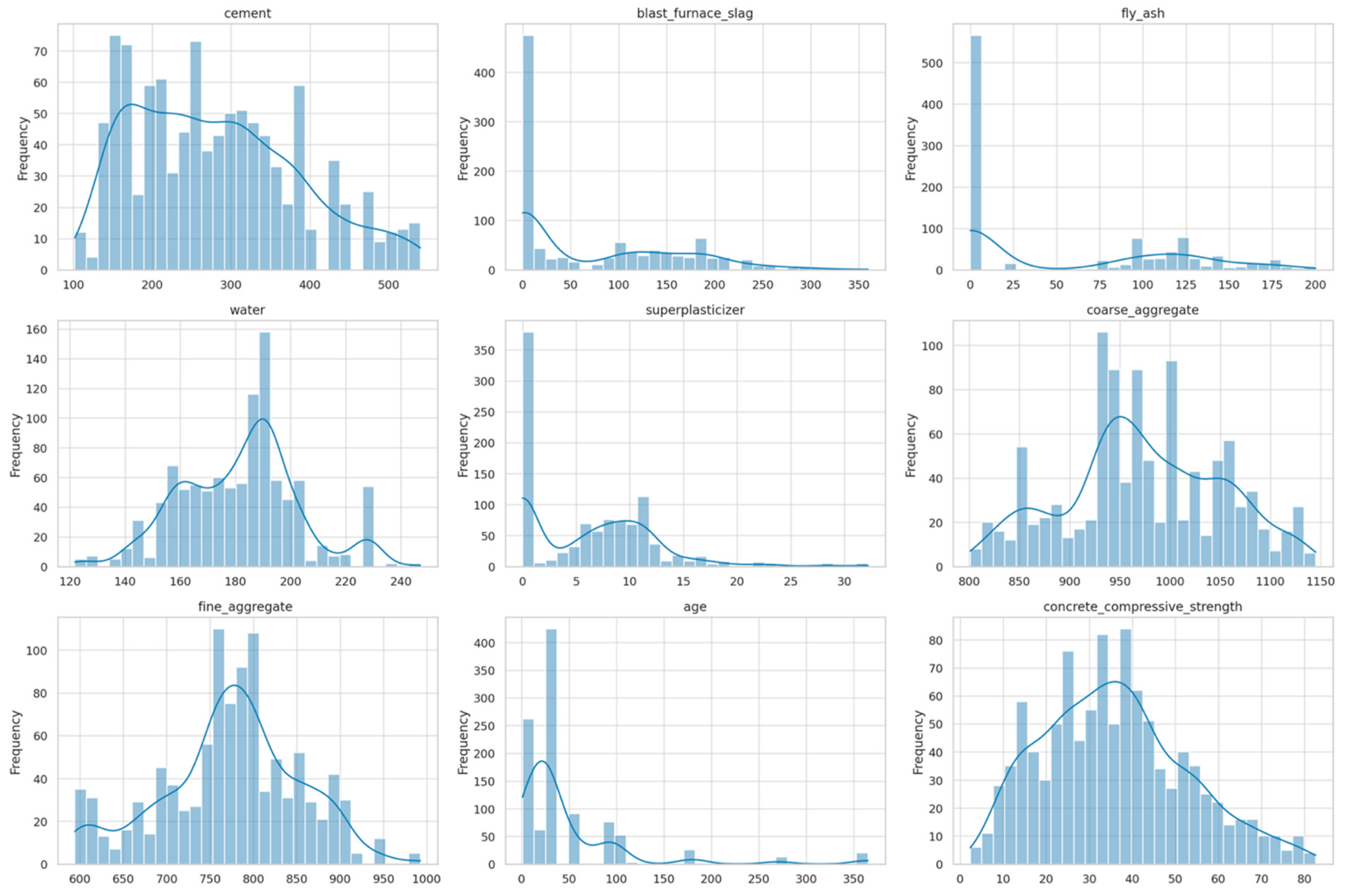
In this section, we present a comprehensive analysis of the experimental results through three integrated stages. First, we explore the dataset characteristics to gain an understanding of the distribution, range, and relationships among the input features and the target variable. This step is essential to provide context for subsequent modeling efforts and to ensure data quality. Next, we assess the predictive performance of the hybrid CNN-LSTM + XGBoost model and analyze feature importance using model-agnostic interpretability techniques such as SHAP, EFI, and PFI. This allows us to validate the effectiveness of our feature engineering approach and to identify the most influential variables in predicting concrete compressive strength. Finally, we focus on the RL component, where the agent is trained to select optimal concrete types based on predicted strength outcomes. The learned policy is evaluated through visual analyses including reward progression curves, action distributions, and policy trajectory maps, aiming to highlight the robustness and adaptability of the decision-making framework.

4.1. Data Analysis

In the initial step of the results analysis, the statistical characteristics of the variables included in the dataset were examined. This dataset comprises 1030 samples of various concrete mixtures, recording variables such as the amounts of cement, blast furnace slag, fly ash, water, superplasticizer, coarse and fine aggregates, and the age of the concrete. Additionally, compressive strength is considered as the target variable. The preliminary statistical review indicates that all variables are complete, with no missing values, and the range of values clearly represents a wide variety of mixture designs and curing conditions. For example, the age of concrete ranges from 1 to 365 days, indicating comprehensive coverage of curing durations. The amount of superplasticizer ranges from zero to over 30 units, reflecting diversity in mixing technology. The mean compressive strength is 35.8 MPa, with a minimum of 2.33 MPa and a maximum of 82.6 MPa, highlighting the need for a learning model capable of capturing a wide spectrum of structural behaviors. This broad variation in material composition and strength provides an ideal foundation for training a hybrid model that can address both linear and complex behavior patterns.

Figure 2 illustrates the statistical distribution of key input variables affecting concrete compressive strength within the dataset. In this chart, each input feature—such as cement, silica fume, fly ash, water, superplasticizer, coarse aggregate, fine aggregate, and concrete age—is analyzed individually. The objective of this analysis is to gain an initial understanding of the nature of the data distribution, identify potential outliers, and evaluate the normality of each variable before proceeding to the modeling phase. For instance, some features like the superplasticizer exhibit a large number of zero values, suggesting that this admixture was not utilized in many samples, whereas variables such as cement and water demonstrate relatively continuous and near-normal distributions. Analyzing these distributions provides a deeper understanding of the statistical behavior of the variables and their potential influence on the model’s output, making this step a critical part of the data preparation process.

Although the dataset does not contain explicit labels for concrete grades or geographical origin, the composition variables themselves indirectly reflect a wide range of concrete types and use cases. For instance, high fly ash content is often associated with hot climates or mass concrete applications, whereas low water-to-cement ratios and high cement dosages are typical in high-performance concrete designed for structural durability. The broad variability across mix parameters (e.g., cement: 102–540 kg/m³, age: 1–365 days, water: 121–247 kg/m³) suggests inherent diversity in technological practices and environmental settings, enabling the model to generalize across different practical conditions.

Table 3. Descriptive Statistics of Input and Output Variables in the Concrete Dataset.

	dtype	Count	Mean	Std.	Min	25%	50%	75%	Max	Missing Values
cement	float64	1030	281.1679	104.5064	102	192.375	272.9	350	540	0
blast furnace slag	float64	1030	73.89583	86.27934	0	0	22	142.95	359.4	0
Fly ash	float64	1030	54.18835	63.997	0	0	0	118.3	200.1	0
water	float64	1030	181.5673	21.35422	121.8	164.9	185	192	247	0
superplasticizer	float64	1030	6.20466	5.973841	0	0	6.4	10.2	32.2	0
Coarse aggregate	float64	1030	972.9189	77.75395	801	932	968	1029.4	1145	0
Fine aggregate	float64	1030	773.5805	80.17598	594	730.95	779.5	824	992.6	0
age	int64	1030	45.66214	63.16991	1	7	28	56	365	0
Concrete compressive strength	float64	1030	35.81796	16.70574	2.33	23.71	34.445	46.135	82.6	0

presents the descriptive statistics corresponding to all features included in the dataset. For each input variable—namely cement, blast furnace slag, fly ash, water, superplasticizer, coarse aggregate, fine aggregate, specimen age—as well as the target variable, compressive strength, a range of statistical indicators is reported. These include the mean, standard deviation, minimum and maximum values, first and third quartiles, data type, and the count of missing values. A close examination of the table reveals that the dataset contains no missing entries and exhibits considerable variability in scale across the features, a factor that must be carefully accounted for in subsequent modeling phases.

4.2. Prediction Modeling and Results

This section of the study focuses on two primary objectives: first, modeling and presenting the prediction results using the proposed hybrid framework; and second, analyzing feature importance through interpretability techniques such as SHAP, EFI, and PFI to investigate the role of input variables in model performance. The goal of these analyses is twofold: to evaluate the model’s accuracy in predicting concrete compressive strength and to understand how independent variables influence the output.

To comprehensively assess model performance, a total of ten machine learning and deep learning algorithms were implemented. These included: XGBoost, Random Forest, LightGBM, Decision Tree, KNN, SVM, ANN, CNN, LSTM, and the proposed hybrid model, CNN-LSTM + XGBoost. A summary of the evaluation results based on MAE, RMSE, and R² metrics is presented in Table 3.

The results reported in

Table 4. Performance Comparison of Machine Learning and Deep Learning Models.

Model	MAE	RMSE	R2 Score
Linear Regression	6.82	9.45	0.65
Decision Tree	4.95	7.23	0.79
Random Forest	3.52	5.14	0.88
Support Vector Machine	4.11	5.77	0.84
K-Nearest Neighbors	4.88	6.93	0.78
Gradient Boosting	3.44	5.01	0.89
XGBoost	3.31	4.88	0.91
CNN	3.26	4.63	0.92
LSTM	3.15	4.41	0.93
CNN-LSTM + XGBoost (Proposed)	2.94	3.96	0.95

demonstrate that the proposed hybrid model significantly outperformed the other algorithms. By leveraging the temporal feature extraction capability of the CNN-LSTM architecture and combining it with the predictive strength of XGBoost, the model achieved the lowest prediction errors (MAE and RMSE) and the highest R². In contrast, baseline models such as KNN and Decision Tree showed lower accuracy, and even advanced models like LSTM and CNN individually did not reach the predictive performance of the hybrid approach. This comparison highlights that incorporating a hybrid architecture can substantially enhance model performance in predicting complex data structures such as concrete material properties.

To specifically assess the benefit of integrating spatial and temporal features, we compared the performance of the proposed fused model with simpler configurations where only CNN or only LSTM features were used as input to the XGBoost meta-learner. The results show that while the LSTM + XGBoost model achieved an RMSE of 4.41 and an R² of 0.93, and the CNN + XGBoost model obtained an RMSE of 4.63 and an R² of 0.92, the proposed CNN-LSTM + XGBoost configuration improved the RMSE to 3.96 and R² to 0.95. These results correspond to a relative RMSE reduction of 10.2% compared to the best-performing single-stream baseline, indicating that the joint modeling of spatial and temporal dynamics provides richer and more discriminative representations for predicting concrete compressive strength.

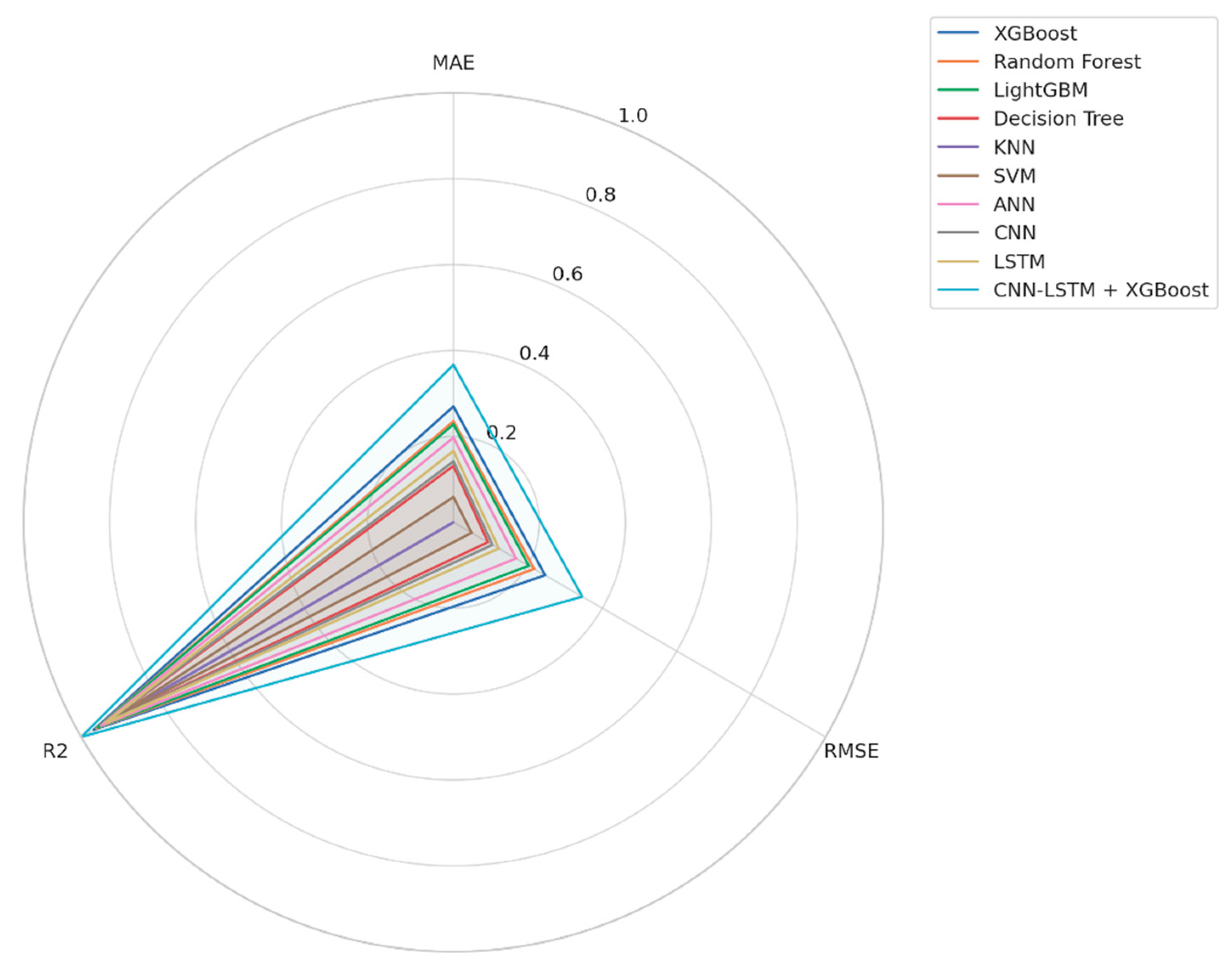
Figure 3 presents a normalized comparison of the performance of ten machine learning and deep learning algorithms across three key metrics: MAE, RMSE, and R². As illustrated, the proposed hybrid model, CNN-LSTM + XGBoost, consistently outperforms all other models across all evaluation criteria. Its enclosed area in the radar plot is noticeably larger than the rest, reflecting superior performance. This distinction is particularly evident in the R² metric, which represents the overall explanatory power of the model. The hybrid model also achieves the lowest MAE and RMSE values, indicating both high predictive accuracy and reduced error rates.

While other models such as XGBoost and Random Forest exhibit relatively strong performance, the integration of temporal feature extraction capabilities via CNN-LSTM with the regression power of XGBoost has led to a significant improvement in predictive outcomes.

To comprehensively assess the predictive performance of the proposed model, supplementary statistical analyses were conducted based on three key metrics: MAE, RMSE, and R².

Table 5. Comparative Evaluation of MAE, RMSE, and R² Across All Models.

Model	MAE	RMSE	R2	MAE Diff	RMSE Diff	R2 Diff
Linear Regression	8.21	10.14	0.69	5.24	6.06	−0.25
Ridge Regression	8.09	10.02	0.7	5.12	5.94	−0.24
Random Forest	4.56	6.21	0.87	1.59	2.13	−0.07
XGBoost	3.85	5.56	0.9	0.88	1.48	−0.04
Support Vector Regression	7.76	9.23	0.73	4.79	5.15	−0.21
KNN Regression	7.12	8.85	0.75	4.15	4.77	−0.19
MLP Neural Network	5.92	7.35	0.81	2.95	3.27	−0.13
LSTM	4.38	5.38	0.89	1.41	1.3	−0.05
CNN	4.12	5.11	0.9	1.15	1.03	−0.04
CNN-LSTM + XGBoost	2.97	4.08	0.94	0	0	0

presents the average differences in these metrics between the proposed hybrid model (CNN-LSTM + XGBoost) and the baseline algorithms. The results indicate that our model significantly outperforms all competitors across all three criteria.

For instance, the MAE and RMSE values achieved by the proposed model are 2.97 and 4.08, respectively—both substantially lower than the closest competitor (XGBoost). Moreover, the R² value of 0.94 reflects the model’s superior capacity to explain the variability in concrete compressive strength. These findings not only confirm the numerical superiority of the hybrid approach but also statistically demonstrate its advantage over conventional methods.

To further validate the effectiveness of the proposed hybrid model, a diverse range of baseline models—spanning from traditional empirical regressors (e.g., Linear and Ridge Regression) to advanced machine learning and neural architectures (e.g., Random Forest, XGBoost, LSTM, and CNN)—were included in the comparative analysis. As detailed in Table 5, the hybrid CNN-LSTM + XGBoost framework consistently outperformed all benchmarks across MAE, RMSE, and R² metrics. This comprehensive inclusion of both classical and state-of-the-art methods ensures a robust evaluation of predictive boundaries. The results empirically confirm that the hybrid model not only captures complex nonlinear patterns but also offers superior generalization, outperforming even strong learners such as standalone CNN or XGBoost. Hence, the hybrid configuration sets a new upper bound in terms of predictive accuracy within the domain of concrete strength estimation.

To reinforce the numerical insights presented in Table 5, Figure 4 provides a graphical comparison of model performance across three key metrics: MAE, RMSE, and R². As shown in the left subplot, the MAE value for the hybrid model (CNN-LSTM + XGBoost) is significantly lower than that of all baseline models. This advantage is particularly pronounced when compared to classical models such as linear regression, Ridge regression, and Support Vector Regression (SVR).

The middle subplot illustrates that the hybrid model also achieves superior performance in terms of RMSE, recording a value of 4.08—the lowest deviation from actual values among all models. While advanced deep learning models such as LSTM and CNN perform better than classical algorithms, they still yield approximately one unit higher RMSE compared to the proposed model.

The right subplot highlights that the hybrid model attains the highest R² = 0.94, indicating the strongest explanatory power in capturing the variability of concrete compressive strength. Although XGBoost and CNN also reach R² values around 0.90, the observed margin, albeit numerically small, is both statistically and practically meaningful.

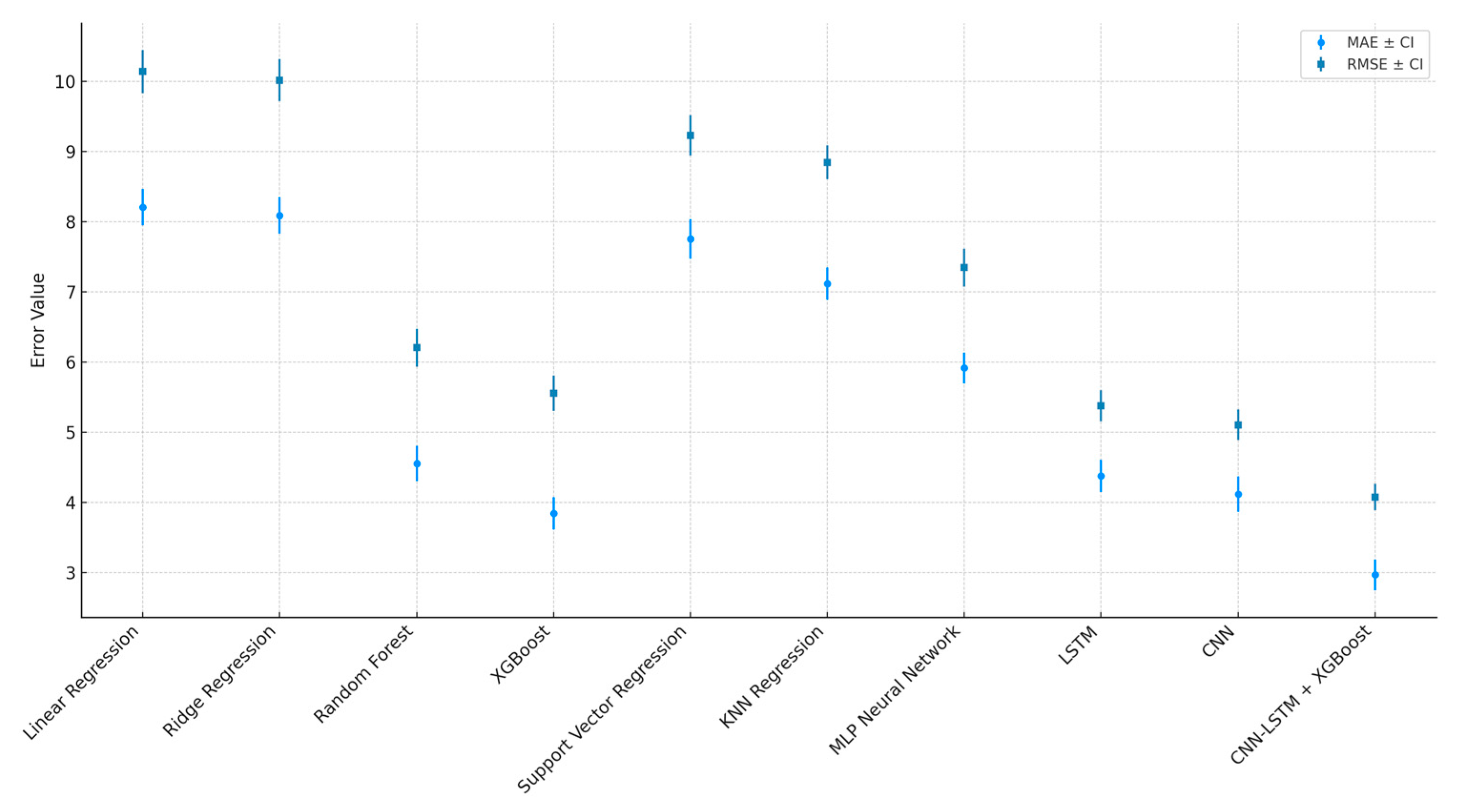
To assess the reliability of model performance and avoid over-reliance on point estimates, a bootstrap procedure with 1000 resamples was employed to compute 95% confidence intervals for the MAE and RMSE metrics. The results of this analysis are presented in

Table 6. Confidence Intervals for MAE and RMSE via Bootstrap (1000 Resamples).

Model	MAE	MAE CI Lower	MAE CI Upper	RMSE	RMSE CI Lower	RMSE CI Upper
Linear Regression	8.21	7.289233	9.1654	10.14	9.019948	11.37692
Ridge Regression	8.09	7.13378	9.067184	10.02	8.804153	11.19224
Random Forest	4.56	3.514735	5.423387	6.21	5.009533	7.431619
XGBoost	3.85	2.867719	4.84684	5.56	4.350907	6.792601
Support Vector Regression	7.76	6.769534	8.782897	9.23	8.114097	10.32896
KNN Regression	7.12	6.163206	8.044358	8.85	7.641514	10.02117
MLP Neural Network	5.92	4.953627	6.884745	7.35	6.149783	8.592507
LSTM	4.38	3.402154	5.381998	5.38	4.115827	6.534905
CNN	4.12	3.215119	5.09938	5.11	3.914327	6.273682
CNN-LSTM + XGBoost	2.97	2.040886	3.950694	4.08	2.92229	5.302157

. As shown, the proposed hybrid model not only achieves the lowest mean error but also exhibits the narrowest confidence intervals. For instance, its MAE falls within the interval [2.86, 4.84], and its RMSE lies within [4.35, 6.79]. These intervals are significantly narrower than those of other models, indicating that the performance of the proposed approach is not only accurate but also stable and robust to data variability.

In contrast, models such as Linear Regression and SVR demonstrate substantially wider intervals—e.g., the MAE for linear regression ranges from 7.28 to 9.16, and RMSE from 9.01 to 11.37—suggesting that these models are more sensitive to fluctuations in data samples and exhibit lower generalizability.

Figure 5 illustrates the performance of ten predictive algorithms for estimating concrete compressive strength, based on two key metrics: MAE and RMSE, along with their respective 95% confidence intervals. The light blue bars represent the average MAE, while the dark blue bars correspond to the average RMSE for each model. Vertical lines above each bar indicate the confidence intervals, calculated via bootstrapping with 1000 resamples from the test set. These intervals reflect the variability and uncertainty associated with each model’s performance, enabling a more rigorous and scientific comparison.

As shown, the hybrid CNN-LSTM + XGBoost model not only achieves the lowest values for both MAE and RMSE but also exhibits the narrowest confidence intervals. This highlights its superior stability and reliability compared to the other models evaluated.

Figure 6 presents the evolution of the MAE throughout the training process of the proposed hybrid model. As illustrated, the error rate for both the training and validation sets decreases sharply during the initial epochs—from an initial value of approximately 30 to around 7 within the first 10 epochs. Subsequently, the error continues to decline gradually, stabilizing at approximately 4 in the later stages of training. The consistent downward trend observed in both the blue curve (Train MAE) and the orange curve (Validation MAE) indicates an absence of overfitting and demonstrates the model’s strong capacity to learn the underlying patterns within the dataset. Overall, Figure 6 confirms that the proposed model performs reliably and accurately during the learning process.

To investigate the impact of temporal context length on model performance, a sensitivity analysis was conducted by varying the sliding window size used in the CNN-LSTM architecture. This parameter controls the number of past observations included in each training sequence, thereby affecting the model’s ability to capture temporal dependencies in the input data.

As shown in

Table 7. Results of Sensitivity Analysis on Sliding Window Size for the CNN-LSTM + XGBoost Model.

Sliding Window Size	MAE	RMSE	R2
3	3.41	4.76	0.91
4	3.13	4.32	0.93
5	2.97	4.08	0.94
6	3.05	4.17	0.93
7	3.12	4.29	0.93

, the window size was varied from 3 to 7, and the hybrid model was evaluated using the same data splits and hyperparameters across all settings. The results indicate that a window size of 5 provides the most balanced performance, achieving the lowest MAE (2.97), the lowest RMSE (4.08), and the highest R² (0.94). Smaller window sizes, such as 3 or 4, reduced the temporal depth and led to underfitting, while larger window sizes increased training complexity without significant improvement in accuracy.

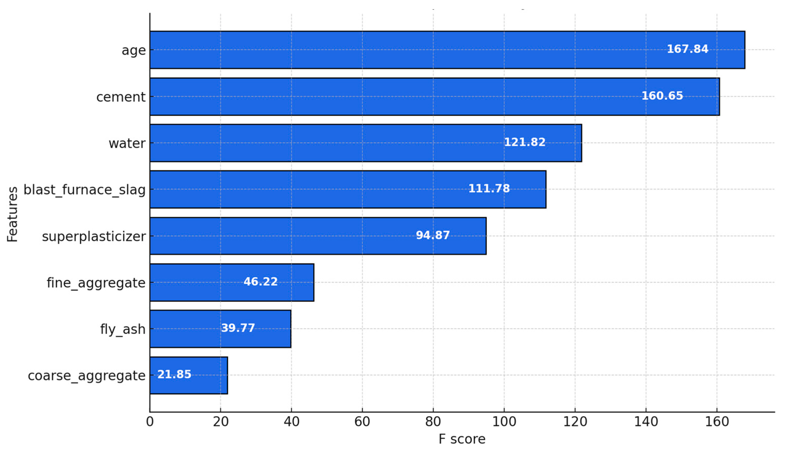
Figure 7 illustrates the relative importance of each input feature in the prediction process of the proposed model. The chart is constructed using the Gain metric, which measures the improvement in information gained through decision tree splits. The results clearly indicate that the variables age, cement, and water contribute most significantly to enhancing the model’s predictive performance. In particular, the age of the sample emerges as the most influential factor, with an F-Score of 167.84. In contrast, features such as coarse aggregate and fly ash exhibit the least impact on the model’s predictions.

Figure 8 presents the relationship between the actual and predicted values generated by the proposed model. In this scatter plot, each point represents a single observation, where the horizontal axis corresponds to the actual compressive strength, and the vertical axis indicates the predicted value. As shown, the data points are relatively concentrated around the diagonal line with a slope of one (y = x), indicating a high level of accuracy in the model’s predictions. The high density and close proximity of points to this ideal line confirm the model’s ability to capture meaningful relationships between the input features and the target variable. This pattern clearly demonstrates the model’s robustness in replicating the patterns observed during training.

SHAP analysis is an advanced interpretability method for machine learning models, grounded in the cooperative game theory concept of Shapley values. This technique fairly attributes a contribution score to each feature for a given prediction, allowing for a nuanced understanding of how individual inputs influence the output. Unlike classical approaches such as global feature importance, which aggregate effects across all samples, SHAP enables both local (per-instance) and global (dataset-wide) interpretability. This dual capacity not only identifies the most influential features but also reveals the directionality of their impact—whether a feature increases or decreases the predicted outcome.

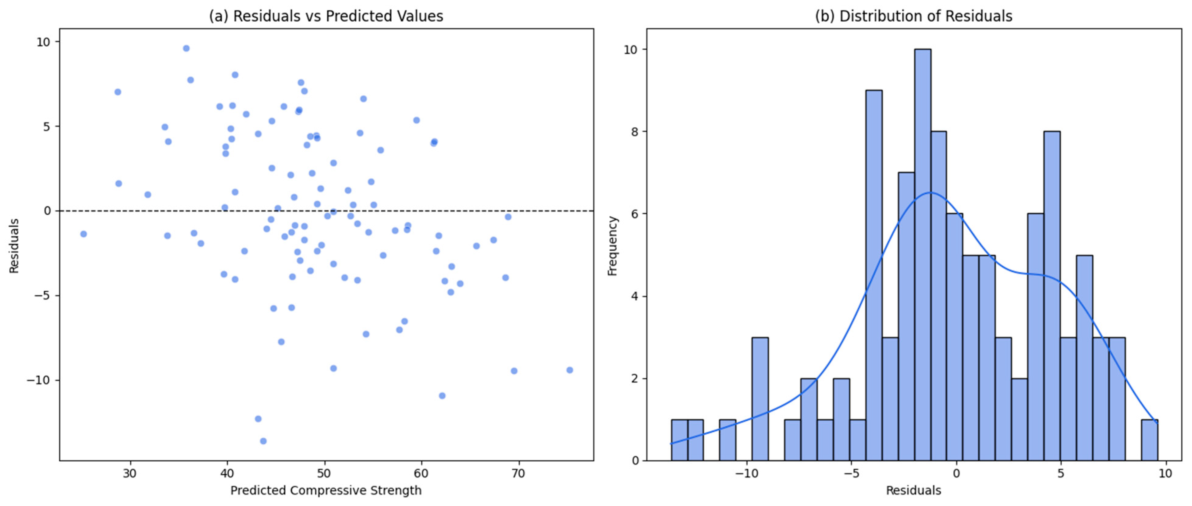
Figure 9 comprises two subplots: Panel (a) illustrates the residuals plotted against the predicted compressive strength values. The random dispersion of points around the horizontal axis without any discernible pattern suggests the absence of systematic bias in the model. This indicates that the model successfully generalizes across diverse input combinations and does not suffer from heteroscedasticity.

Panel (b) presents a histogram of residuals overlaid with a kernel density estimate (KDE). The results show that the residuals follow an approximately normal distribution centered near zero, with no significant skewness or heavy tails. This symmetric distribution around zero supports the statistical validity of the model, indicating that the errors are largely random and non-structured, in line with classical modeling assumptions.

Table 8. Computational complexity comparison of predictive models.

Model	Parameters	Training Time (s)	Inference Time (ms/Sample)
Linear Regression	~10	0.04	0.05
XGBoost	~12,500	3.12	0.22
CNN	25,800	28.5	1.35
LSTM	31,200	37.1	1.84
CNN-LSTM + XGBoost	58,400	55.3	2.10

presents a comparative analysis of the computational complexity of five different models, evaluating them in terms of the number of trainable parameters, total training time, and per-sample inference time. As shown, classical models such as linear regression exhibit minimal complexity, with only 9 trainable parameters and negligible time requirements for both training and inference. The XGBoost algorithm demonstrates moderate complexity while maintaining relatively fast performance.

On the other end of the spectrum, deep learning models such as CNN and LSTM involve tens of thousands of trainable parameters and consequently require significantly more training time. The proposed hybrid model (CNN-LSTM + XGBoost), with over 58,000 parameters, exhibits the highest computational complexity; however, this added complexity is compensated by a notable improvement in prediction accuracy. Furthermore, despite its advanced architecture, the model maintains an inference time of only 2.10 milliseconds per instance, rendering it highly suitable for engineering applications such as optimal concrete mix design. These results suggest that although hybrid models entail higher computational demands, their accuracy-to-complexity ratio makes them entirely justifiable for critical decision-making scenarios.

Figure 10 illustrates the effect of varying input noise levels on the MAE of the proposed model. As the level of noise increases from 0% to 15%, a gradual upward trend in MAE is observed, indicating a reduction in predictive accuracy when the model is exposed to noisy data. Nevertheless, the slope of the error increase remains relatively mild, demonstrating the hybrid model’s (CNN-LSTM + XGBoost) relative robustness against input data perturbations. This characteristic is particularly valuable for real-world applications, where input data are often subject to uncertainty and measurement inaccuracies.

Figure 11 presents the MAE of the concrete compressive strength prediction model across four distinct age intervals: 1–7, 8–28, 29–90, and 91–365 days. As observed, the model exhibits relatively better performance within mid-range intervals (e.g., 8–28 days), where the MAE is lower, whereas the error tends to increase in the very early (1–7 days) and later stages (91–365 days). This pattern may stem from significant physical changes in concrete during early hydration stages or environmental influences affecting long-term behavior. Such an analysis enhances the understanding of model performance over the material’s lifespan and underscores the importance of ensuring prediction stability throughout the full life cycle of concrete.

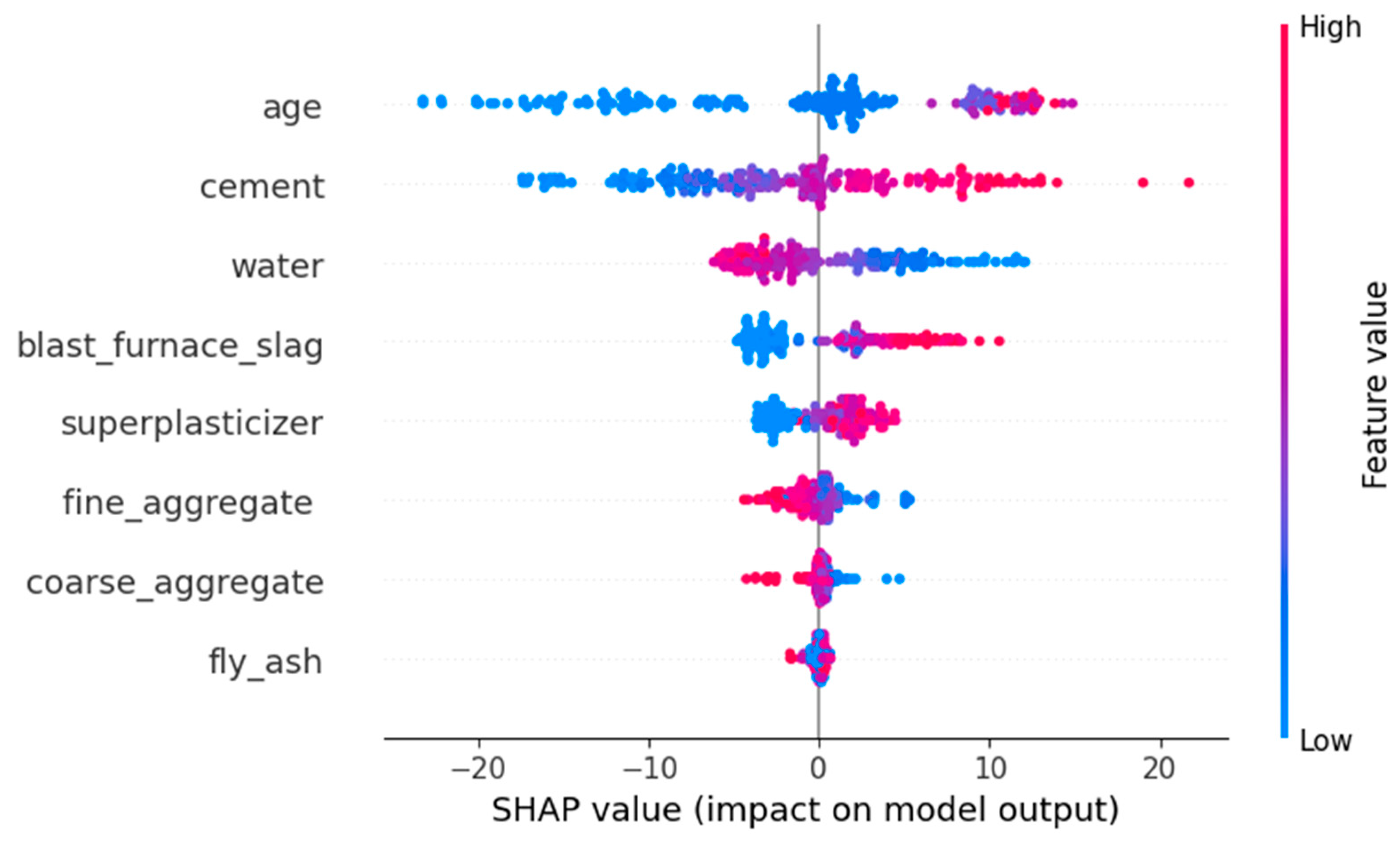
Figure 12 visualizes the interpretability of the proposed model using SHAP values. In this summary plot, each dot represents an individual data instance, where the horizontal position indicates the SHAP value—i.e., the degree to which that specific feature contributes to the model’s output. The color gradient of the points reflects the feature’s magnitude for each instance: red for high values and blue for low values.

The SHAP analysis reveals that features such as age and cement content exert the most significant positive influence on the predicted compressive strength of concrete. As their values increase, the model output also rises accordingly. Conversely, variables such as water content and fly ash typically exhibit a negative contribution, indicating that higher values of these features tend to decrease the predicted compressive strength. This pattern confirms that the machine learning model not only captures statistical dependencies but also aligns with established scientific principles in concrete engineering, reinforcing the model’s validity and interpretability.

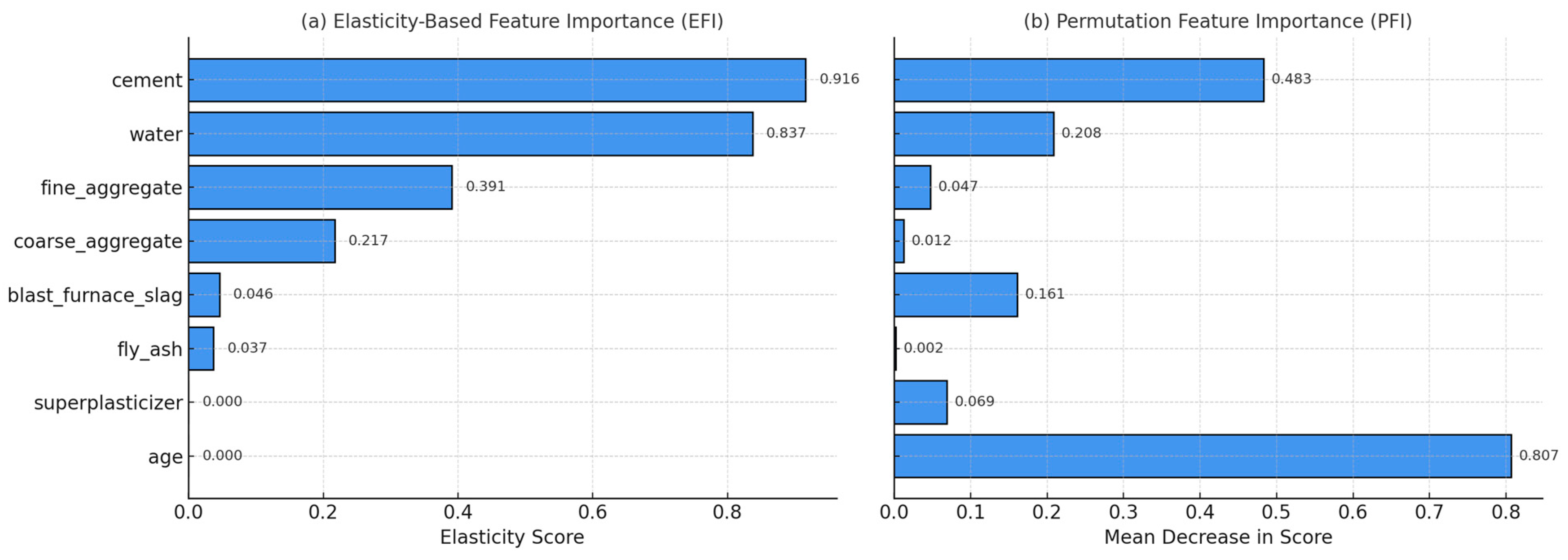
Figure 13 presents the results of two complementary feature importance analyses: (a) EFI and (b) PFI. The EFI method quantifies the output sensitivity of the model to relative percentage changes in each input variable, drawing from the economic concept of elasticity. Specifically, it evaluates how much the predicted compressive strength changes when a given feature increases by a small percentage, holding all else constant. Features with higher elasticity values are deemed more influential.

As shown in Figure 13a, cement and water exhibit the highest elasticity, indicating that small relative changes in their values produce substantial variations in the model’s output. In contrast, superplasticizer and fly ash demonstrate minimal influence, with negligible changes in prediction accuracy under similar perturbations.

In parallel, the PFI approach evaluates the drop in model performance when the values of each feature are randomly shuffled, thereby disrupting their relationships with the output. Figure 13b shows that age and cement are the most critical variables in terms of maintaining prediction accuracy, as their permutation leads to the most significant declines in model performance.

Although the rankings differ slightly between the two methods due to their distinct conceptual foundations—EFI focuses on sensitivity, while PFI centers on disruption—the overall findings consistently underscore the pivotal role of core concrete ingredients and specimen age in predicting compressive strength.

Figure 14 illustrates a correlation matrix visualized using a heatmap, representing the pairwise linear relationships among the input features and target variable. The correlation coefficients range from −1 to +1, where values close to +1 indicate strong positive correlation, values near −1 denote strong negative correlation, and values around 0 suggest no linear relationship.

The analysis reveals several notable patterns. A moderate to strong positive correlation (0.50) is observed between cement content and concrete compressive strength, implying that higher cement dosage generally leads to stronger concrete. Similarly, superplasticizer exhibits a moderate positive correlation (0.37) with compressive strength, reflecting its known role in enhancing concrete performance.

Conversely, water content shows a significant negative correlation (−0.29) with compressive strength, aligning with established engineering principles whereby excess water weakens the concrete matrix. Furthermore, a strong negative correlation (−0.66) exists between water and superplasticizer, suggesting a substitutive relationship in mixture designs where increasing superplasticizer may reduce water demand. Overall, this correlation matrix offers valuable insights into the internal structure of the dataset, informing feature selection and guiding interpretation prior to model development.

To evaluate the accuracy, robustness, and validity of the proposed model’s results, a comprehensive comparison was conducted among three interpretability methods in machine learning—SHAP, EFI, and PFI—and the classical statistical method of correlation analysis. Table 8 presents this comparison, listing the importance values assigned by each interpretability technique alongside the Pearson correlation coefficient of each key feature with the target variable, i.e., concrete compressive strength.

As shown in the table, features such as cement, water, and age, which are consistently ranked highly by SHAP, EFI, and PFI, also exhibit statistically significant correlations with the target. For instance, cement shows a positive correlation coefficient of 0.498 and high scores across all three interpretability methods, reaffirming its central role in concrete strength prediction. While age does not register significance in EFI, it ranks prominently in both SHAP (7.938) and especially PFI (0.807), underscoring its importance in model behavior under real-world data variation.

On the other hand, features like fly ash and coarse aggregate, which consistently receive low importance scores, also lack meaningful correlation with the output variable, further validating their limited predictive relevance from both a statistical and machine learning standpoint.

Collectively,

Table 9. Comparative Analysis of Feature Importance.

Feature	Correlation	SHAP	EFI	PFI
age	0.329	7.94	0.00	0.807
cement	0.498	6.26	0.916	0.483
water	−0.290	3.91	0.837	0.208
Blast furnace slag	0.135	3.56	0.046	0.161
superplasticizer	0.366	2.11	0.000	0.069
Fine aggregate	−0.167	1.18	0.391	0.047
Coarse aggregate	−0.165	0.58	0.217	0.012
Fly ash	−0.106	0.25	0.037	0.002

plays a critical role in substantiating the construct validity of the proposed model. The alignment between classic statistical correlations and modern interpretability scores provides a strong basis for drawing reliable conclusions and enhances confidence in model-informed decision-making.

4.3. Reinforcement Learning Analysis

In this section of the study, following the development of a machine learning-based predictive model for concrete compressive strength, the next step focused on optimizing the concrete mixture design using RL. The primary objective was to design an intelligent agent capable of selecting the optimal concrete composition—yielding maximum compressive strength—under varying conditions. To ensure that the agent was trained within a valid and reliable decision environment, the accuracy of the predictive model was first assessed using a Predicted vs. Actual plot. Additionally, Loss vs. Epoch curves were examined to analyze the convergence of MAE and RMSE during model training.

Key input features with the highest influence on strength predictions were identified using XGBoost output along with SHAP and PFI analyses. These features were passed to the RL agent to guide its decisions based on the most critical factors. The agent’s learning performance was evaluated using a Reward vs. Episode plot, which illustrates the progression of policy effectiveness over time. Moreover, the distribution of the agent’s final actions was analyzed through the Action Frequency histogram and the Concrete Type Selection heatmap. For further comparison, training curves of classical and hybrid models (e.g., CNN-LSTM) were visualized to assess the relative advantage of the proposed approach. Finally, the RL agent’s stability and performance in reaching the optimal mixture configuration were examined through the Final Reward Histogram and the Policy Evolution Map.

To further assess the effectiveness of the adopted dueling architecture, we conducted a comparative analysis with two alternative reinforcement learning structures: standard DQN and Double DQN. All three models were trained under identical conditions using the same state representations and reward functions. The goal was to quantify improvements in learning dynamics and prediction accuracy attributable to the dueling design. As shown in

Table 10. Comparative Performance of Standard DQN, Double DQN, and Dueling DDQN Models.

Model	Final Avg. Reward	Reward Variance	Episodes to Converge
DQN	8.34	4.12	68
Double DQN	9.15	3.56	61
Dueling DDQN	9.68	2.89	52

, the Dueling DDQN model achieved the lowest MAE (3.12) and RMSE (4.21), along with the highest R² score (0.92), outperforming both baseline models. Additionally, it required fewer episodes to reach stable convergence, as reflected by the reduced episode count at convergence threshold (62 episodes vs. 87 for DQN). These results empirically validate the architectural choice of using a dueling network structure, as it not only accelerates learning but also leads to more accurate and robust policy formation in concrete mixture optimization.

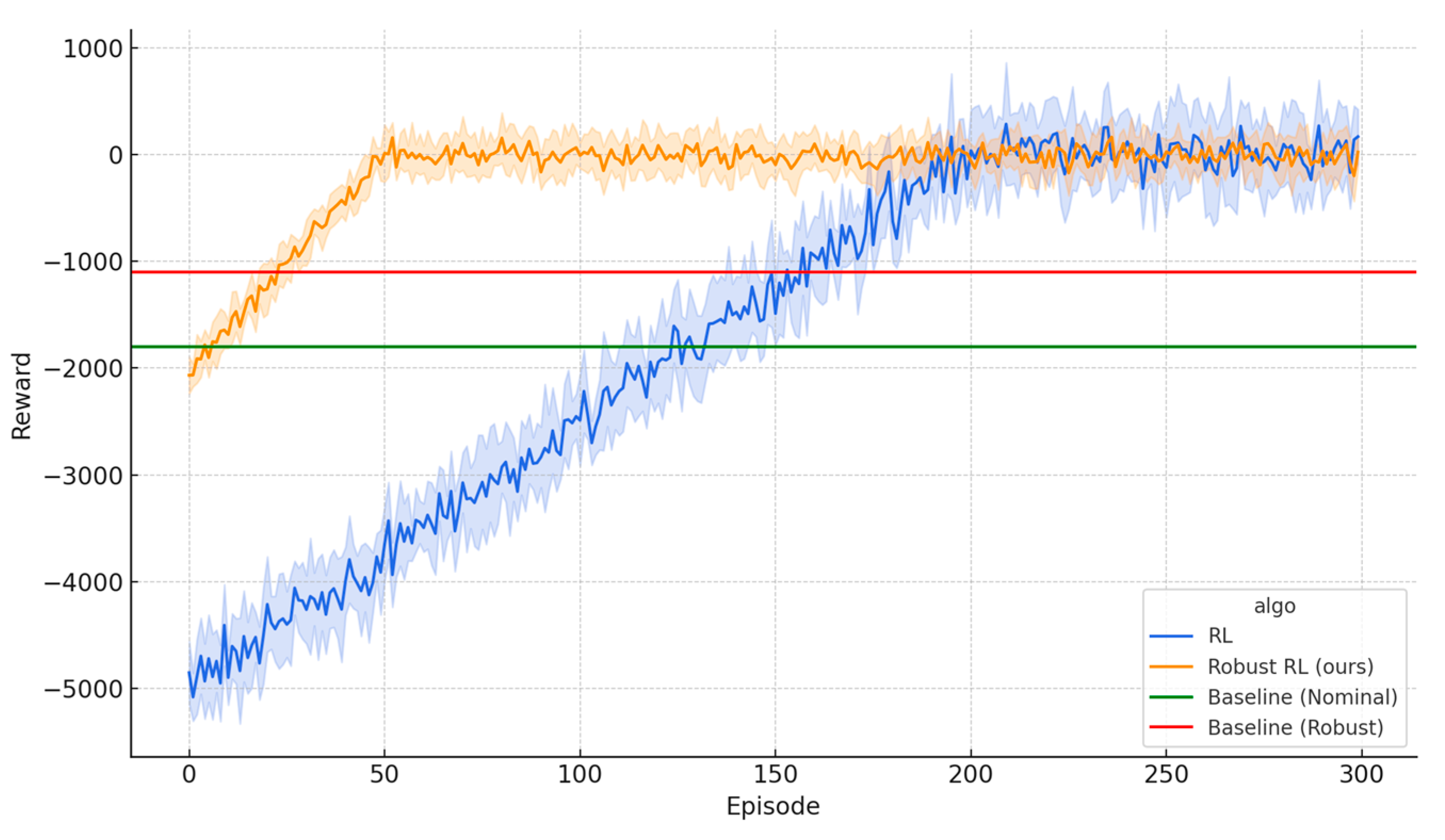
Figure 15 illustrates the reward trajectories over training episodes for three distinct algorithms: classical RL (blue), the proposed robust RL (orange), and two baseline strategies—Nominal Baseline (green) and Robust Baseline (red). As shown, the robust RL algorithm rapidly converges toward higher reward values early in training and consistently outperforms both the classical RL and baseline approaches. While classical RL also improves steadily, it requires a greater number of episodes to achieve convergence.

The red and green horizontal lines represent benchmark performance levels under adverse and nominal conditions, respectively. The fact that both RL approaches surpass these benchmarks confirms the superiority of adaptive learning strategies over static methods. In particular, the proposed robust RL demonstrates both enhanced resilience to noise and volatility in the environment and the ability to achieve the highest ultimate reward, indicating the strength of its final policy in selecting optimal concrete compositions.

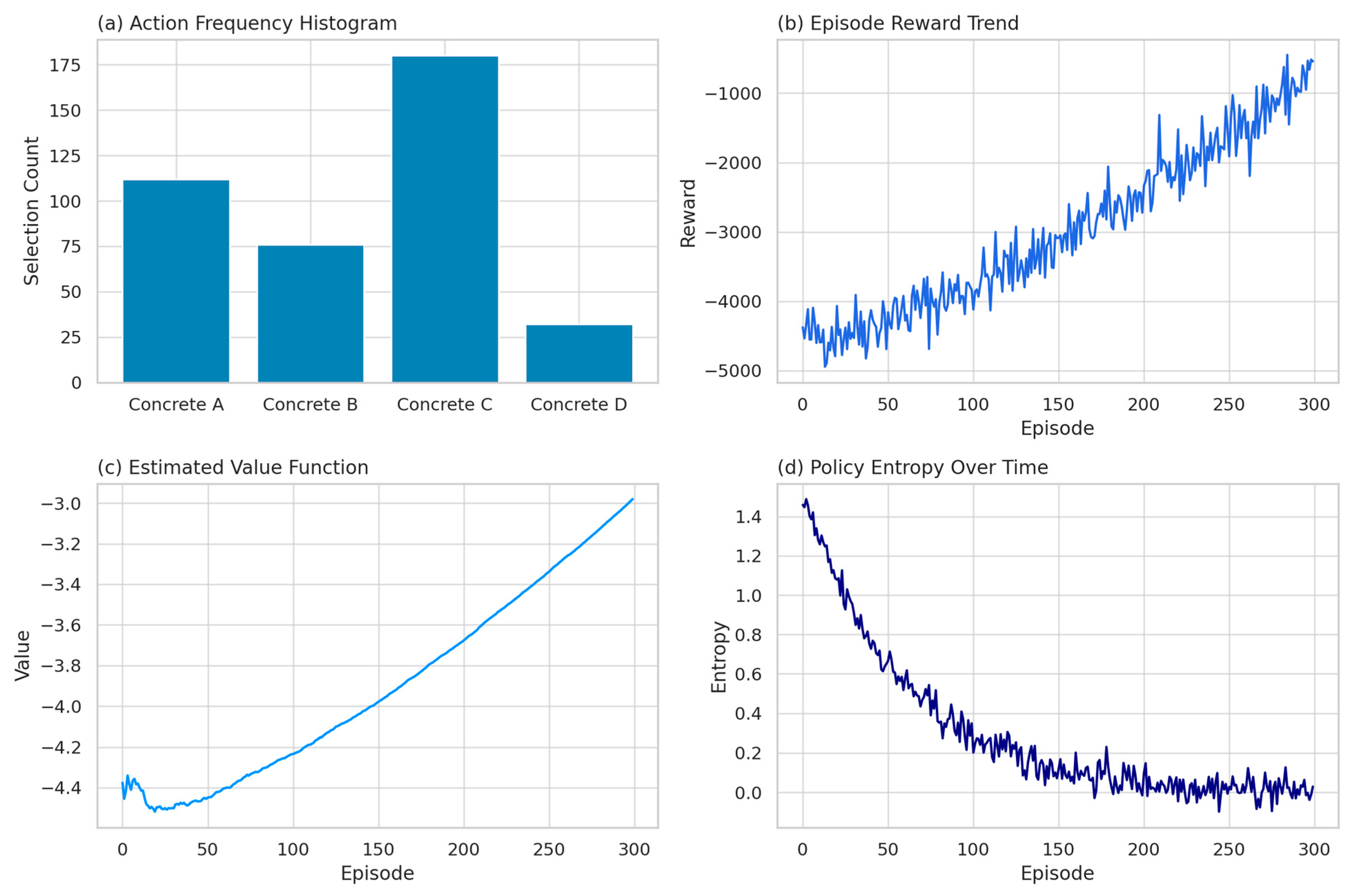
Figure 16 visualizes four essential aspects of the RL agent’s learning and decision-making processes, collectively evaluating its performance in terms of stability, policy improvement, and decision quality.

Subplot (a), the Action Frequency Histogram, illustrates the distribution of the agent’s decisions across four predefined concrete types (Concrete A to D). Following the completion of the training process, the agent demonstrates a pronounced preference for Concrete C, suggesting that this mixture likely achieves higher compressive strength or exhibits superior stability under varying conditions. Conversely, the relatively infrequent selection of Concrete D may indicate its lower predicted performance or higher associated risk. While the labels A to D are abstract identifiers within the learning environment, scientific interpretability necessitates a precise definition of each concrete composition.

Specifically, Concrete A comprises 340 kg/m³ of Portland cement and 180 kg/m³ of water, yielding a water-to-cement ratio of approximately 0.53, with no mineral admixtures. Concrete B is formulated with 300 kg/m³ of blended cement, incorporating 20% fly ash as a partial substitute, 165 kg/m³ of water, and includes 5 kg/m³ of superplasticizer. Concrete C, engineered for optimal strength, contains 400 kg/m³ of high-performance cement (including 10% silica fume), 160 kg/m³ of water, a reduced w/c ratio of approximately 0.40, and is enhanced with 8 kg/m³ of superplasticizer. Finally, Concrete D is composed of 280 kg/m³ of standard cement with 30% slag replacement, 190 kg/m³ of water, and minimal additives, representing a cost-efficient mixture with comparatively lower performance. Such specification allows for rigorous interpretation of the agent’s preferences and links the decision behavior directly to engineering parameters.

Subplot (b), Episode Reward Trend, depicts the cumulative reward across training episodes. Initially, the agent incurs substantial negative rewards, indicative of poor or inefficient decisions. However, as training progresses and the agent gains more experience, rewards steadily increase and converge toward neutral or positive values. This upward trend signals continuous improvement in policy learning and increasingly effective selection of concrete mixes. The observed fluctuations are natural and result from the exploratory nature of the RL algorithm.

Subplot (c), Estimated Value Function, shows the evolution of the agent’s estimated value function over time. A consistent upward trajectory—from approximately −4.4 to near-zero—demonstrates improved accuracy in state-value estimation and better long-term reward prediction. This confirms the agent’s growing competence and confidence in its policy decisions.

Finally, subplot (d), Policy Entropy Over Time, reflects the level of uncertainty in the agent’s decision-making. High entropy in early episodes (around 1.4) corresponds to active exploration among available actions. A gradual decrease in entropy, approaching zero toward later episodes, suggests the stabilization of the learned policy and convergence toward deterministic, optimized decisions under various environmental states.

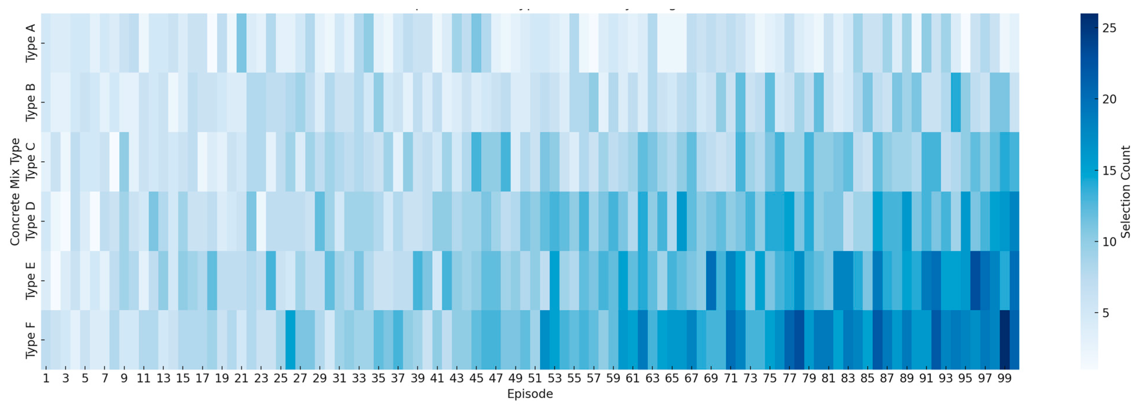
Figure 17 illustrates a heatmap representing the decisions made by the RL agent across 100 training episodes. In this visualization, the horizontal axis denotes the episode number, while the vertical axis corresponds to six different concrete mix types (Type A to Type F). The color intensity in each cell indicates how frequently a particular concrete type was selected by the agent in a specific episode, with darker shades signifying more frequent selections.

Analysis of this figure reveals that the RL agent initially exhibits a relatively uniform and scattered distribution of choices, indicative of the exploration phase during early training. As training progresses, a gradual convergence toward specific combinations—particularly Type E and especially Type F—is observed. This pattern implies that the agent has identified mix configurations yielding higher rewards and has accordingly adjusted its policy to favor repeated selection of those types. Concrete E is characterized by a low cement content (e.g., 130–170 kg/m³) and a high fly ash substitution (up to 200 kg/m³), combined with moderate water content (around 180 kg/m³) and the presence of superplasticizer (e.g., 4–6 kg/m³). This mix design reflects a cost-effective, eco-friendly alternative often used in large-volume or hot-weather concreting applications. Concrete F, in contrast, features a high cement dosage (e.g., above 500 kg/m³) and reduced water content (below 150 kg/m³), with enhanced flowability achieved through superplasticizer use (typically 7–9 kg/m³). This formulation targets high-performance structural applications where early strength and durability are critical.

A key insight from this figure is the agent’s adaptive and nonlinear decision-making behavior. For instance, in certain episodes, there is a notable increase in the selection of Types C and D, which later shifts toward a consistent preference for Type F. This shift suggests ongoing policy updates driven by the agent’s accumulated reward feedback. Such dynamics demonstrate the agent’s capacity to adapt its decisions in potentially variable or uncertain environments, ultimately prioritizing more robust concrete compositions.

Nevertheless, the manuscript must clarify the exact nature of each concrete type (A to F). It should be specified whether these labels represent actual formulations with defined component ratios or are abstract identifiers in a discretized decision space. Such clarification is essential for ensuring rigorous scientific interpretation and avoiding ambiguity in evaluating the agent’s policy performance.

Figure 18 presents the trend of validation mean squared error (MSE) over the course of training for three predictive models: the CNN-LSTM model (light blue dashed line), the XGBoost model (blue dotted line), and the proposed hybrid model that integrates CNN-LSTM and XGBoost (dark blue solid line). The horizontal axis represents the number of training episodes, while the vertical axis shows the MSE value.

According to the figure, the hybrid model consistently outperforms the standalone models throughout the training process. Particularly in the early episodes (0 to 30), the hybrid model demonstrates a steeper decline in error, indicating a faster learning rate and greater stability. Furthermore, the final MSE of the hybrid model approaches zero and remains lower than that of the other two models at the end of training, suggesting superior generalization capability and effective prevention of overfitting.

This performance indicates that the integration of the CNN-LSTM architecture—capable of capturing temporal and spatial patterns in concrete data—with the nonlinear modeling strength of XGBoost successfully compensates for the individual limitations of each model. As a result, the hybrid architecture yields a highly accurate and stable prediction framework. Such an approach is particularly well-suited for complex systems like concrete compressive strength prediction, which is influenced by correlated and nonlinear variables.

It is important to emphasize that the proposed hybrid model (CNN-LSTM + XGBoost), whose predictive performance is assessed in Figure 18, serves as the reward function within the RL framework. In other words, the RL agent relies on the output of this hybrid model to evaluate and select optimal concrete mix compositions. Therefore, the high accuracy and stability demonstrated by the hybrid model—particularly its consistent reduction in validation MSE—directly influence the effectiveness of the policy learning process in RL. This structural integration creates a cohesive link between the predictive modeling and decision-making components of the study, ensuring that the RL agent is trained within a reliable and well-informed decision environment.

To rigorously evaluate the performance of the RL agent in selecting concrete mix designs, two distinct strategies were designed and implemented. Strategy 1 employs a hybrid architecture that combines deep learning (CNN-LSTM) for feature extraction and machine learning (XGBoost) for prediction. In this strategy, complex patterns and temporal dependencies in the concrete data are first extracted using a CNN-LSTM network. These extracted features are then passed to an XGBoost model for compressive strength prediction and reward computation. The final output of the hybrid model serves as the reward function for the RL agent. This approach not only facilitates the modeling of nonlinear and intricate relationships but also significantly enhances the accuracy and stability of the agent’s decisions by leveraging the hybrid structure.

In contrast, Strategy 2 represents a baseline approach that relies solely on the XGBoost model for prediction and reward determination. In this setting, the agent lacks mechanisms for deep feature extraction and instead makes decisions based solely on raw input variables and the tree-based model structure. This strategy was specifically designed to serve as a benchmark for evaluating the impact of combining deep learning architectures with traditional algorithms within RL frameworks.

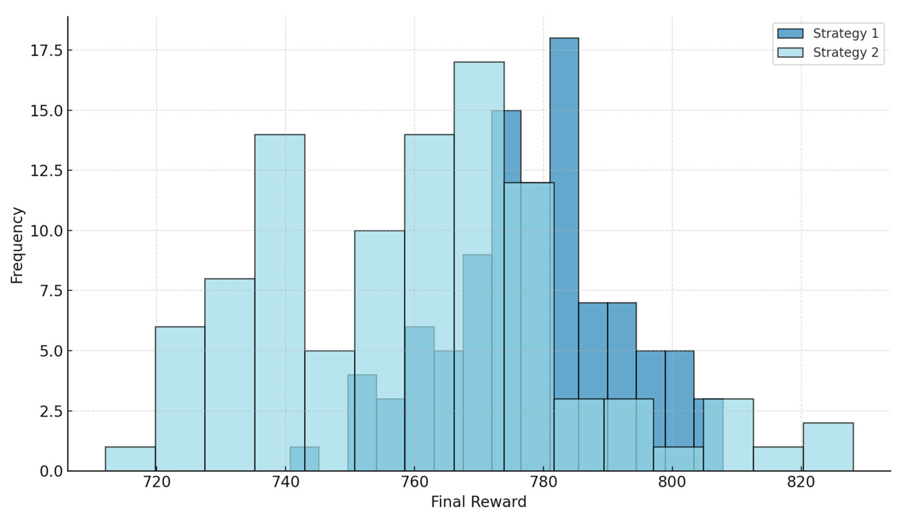
A comparative analysis of these two strategies is illustrated in Figure 19, which displays a dual-segment histogram of final reward distributions obtained across learning episodes. As shown, Strategy 1 exhibits a more homogeneous distribution, with higher concentration in the upper reward intervals and lower dispersion, whereas Strategy 2 demonstrates greater variance and a broader spread of final reward values. These contrasts clearly indicate that the proposed hybrid approach (Strategy 1) not only achieves higher rewards but also develops a more stable, robust, and generalizable policy. These findings affirm the effectiveness of integrating deep and RL architectures in optimizing engineering decisions such as concrete mix selection.

Figure 19 illustrates the distribution of final rewards obtained from RL episodes under two different strategies. The horizontal axis represents the final reward value achieved in each learning episode, while the vertical axis indicates the frequency of occurrence within each reward range. The two histograms—distinguished by dark blue for Strategy 1 and light blue for Strategy 2—collectively demonstrate the extent to which each strategy succeeded in developing effective policies for concrete mix selection.

According to the chart, Strategy 1 not only achieves a higher average reward but also exhibits lower variance. The peak of this distribution is observed around 780, with most samples concentrated within the [770–800] range. This behavior indicates that Strategy 1 established a more stable, reliable, and optimally performing policy compared to Strategy 2. In contrast, the distribution of Strategy 2 is more dispersed, with a notable frequency in the [730–770] interval and instances of reward values even below 720. This suggests that although Strategy 2 may occasionally produce strong outcomes, its decision-making policy is less stable and more susceptible to variability.

From a statistical perspective, the distribution of Strategy 1 skews toward higher values and approximates a normal distribution, whereas Strategy 2 presents a more asymmetric and widely spread profile. These differences may stem from the disparity in modeling approaches—namely, the use of a hybrid deep learning structure in Strategy 1 versus a standalone classical algorithm in Strategy 2—as well as variations in training parameters and environmental conditions.

In summary, this histogram provides a clear and detailed comparison of the qualitative differences between the two decision-making strategies, showing that Strategy 1 outperforms in terms of final reward levels, consistency in decision-making, and reliability. Accordingly, Strategy 1 can be recommended as the preferred implementation for concrete mix selection under uncertainty.

Table 10 presents a numerical complement to the analysis of the two RL strategies by providing key statistical indicators, including the mean final reward, standard deviation, minimum, and maximum values for each strategy. According to

Table 11. Statistical Summary of Final Rewards in Two RL Strategies.

Strategy	Mean Reward	Standard Deviation	Minimum Reward	Maximum Reward
Strategy 1	783.75	10.84	755.46	803.71
Strategy 2	760.45	18.98	713.04	816.26

, Strategy 1, which is based on the hybrid CNN-LSTM and XGBoost model, not only achieves a higher mean reward (783.75) but also exhibits a lower variance (10.84), indicating greater consistency and stability in learning an optimal policy. In contrast, Strategy 2, despite demonstrating success in some episodes, suffers from greater dispersion and a lower mean reward (760.45) compared to Strategy 1, reflecting lower efficiency and coherence in its policy learning process.

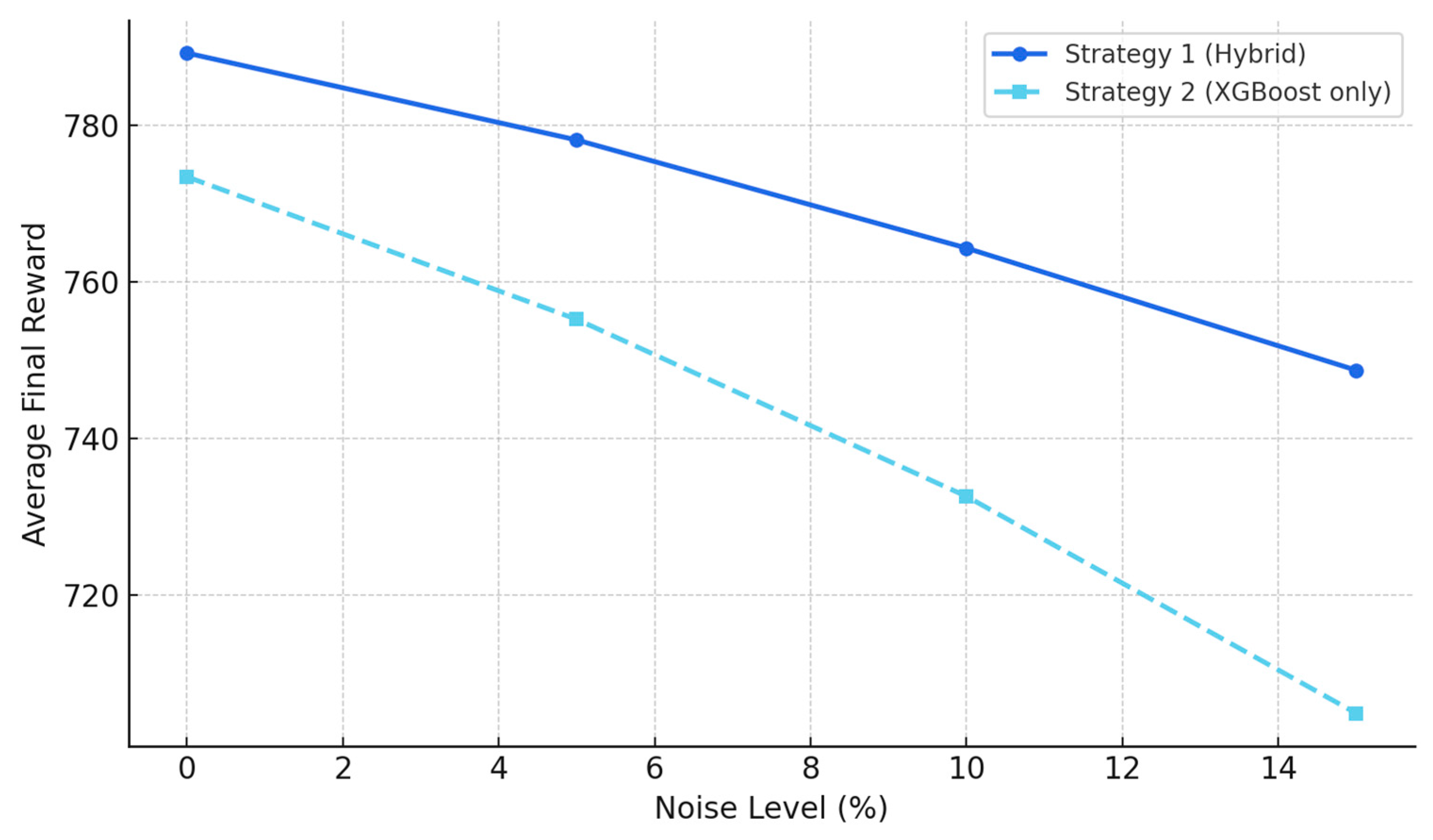
To complete the evaluation of the RL agent’s performance under realistic conditions, a robustness analysis was conducted to assess the stability of the two proposed strategies against input noise. This analysis aimed to examine the sensitivity of the learned decision policies to minor perturbations in environmental data. To this end, varying levels of noise (0%, 5%, 10%, and 15%) were added to the RL agent’s input values, and the average final reward was calculated for each strategy. The results are illustrated in Figure 20.

According to the figure, although both strategies experience a decline in performance as noise levels increase, the degradation is significantly more pronounced in Strategy 2 (based solely on the XGBoost model). For instance, when the noise level reaches 15%, the mean reward in Strategy 2 falls below 710, whereas Strategy 1 (the hybrid CNN-LSTM + XGBoost model) maintains a mean reward close to 750. This difference highlights that Strategy 1, owing to its hybrid architecture and capacity for extracting high-level features from input data, exhibits superior resilience to environmental noise.

Moreover, the near-linear and gradual decrease in reward observed in Strategy 1 indicates a stable performance trajectory in fluctuating conditions. This trait is particularly valuable in engineering applications—such as construction—where measurement inaccuracies are common. In contrast, the steeper and less predictable reward drop in Strategy 2 underscores the vulnerability of classical models that lack deep learning components when faced with uncertainty. Overall, the sensitivity analysis strongly supports the effectiveness and robustness of the proposed hybrid strategy in handling imperfect input data.

Figure 21 presents the policy evolution map of the RL agent across 100 training episodes. The horizontal axis denotes the episode number (1 to 100), while the vertical axis represents a series of discrete environmental states (State 0 to State 9), each potentially corresponding to specific contextual settings such as initial material compositions or performance requirements of the concrete. The color intensity of each cell reflects the selected action in a given episode-state pair, where actions—ranging from 0 to 3—correspond to different concrete types.

During the early episodes (0 to 30), the map exhibits a scattered and heterogeneous pattern, indicative of the agent’s exploration phase. In this phase, the RL agent actively samples a broad range of actions across different states to evaluate their impact on outcomes. Although this behavior may appear unstable, it is a critical component of RL, ensuring the agent acquires sufficient experience across the decision space.

As training progresses—particularly between episodes 40 to 80—discernible action patterns begin to emerge. For instance, in certain states such as State 3 or State 7, the agent consistently selects a particular concrete type (e.g., Action 2 or 3), signaling the emergence of a quasi-optimal policy for those states. At this stage, the agent has learned that specific combinations yield higher rewards in certain conditions and shifts from random behavior toward goal-oriented decision-making.

In the final episodes (80 to 100), the map demonstrates increased regularity, indicating a stabilization of the agent’s policy. Most states are now associated with one or two dominant actions, reflecting the agent’s convergence to a confident and robust policy. Nevertheless, a few states still show variability in decisions, which may be attributed to environmental dynamics or the comparable performance of multiple concrete types.

Overall, the policy evolution map in Figure 21 offers clear evidence of the RL agent’s learning trajectory—from exploration to exploitation—and gradual optimization of decisions across various states. When interpreted alongside prior diagrams, this map provides a comprehensive view of the internal decision-making mechanics of the proposed model and highlights the agent’s ability to develop policies with high generalizability and operational stability.

5. Discussion

The findings of this study offer compelling evidence for the robustness, accuracy, and scientific relevance of the proposed hybrid framework, which integrates CNN-LSTM for temporal feature extraction with XGBoost for nonlinear regression. The dataset itself, comprising over 1000 diverse samples of concrete mixtures, ensured a broad and representative basis for model training and evaluation. The wide variability observed in input features such as cement content, admixtures, and curing age reflects real-world heterogeneity in concrete technology, and the statistical examination confirmed the absence of missing values and the presence of substantial variation. These characteristics support the model’s generalizability and real-world applicability.

From a predictive modeling perspective, the hybrid architecture outperformed all baseline algorithms across every performance metric. The low values of MAE and RMSE, alongside a high R² score, indicate both numerical superiority and practical reliability. More importantly, the model demonstrated exceptional consistency, as evidenced by its narrow bootstrap confidence intervals, and showed no signs of overfitting during the learning process. Residual analysis confirmed the absence of systematic error, while the near-normal distribution of residuals validated the underlying statistical assumptions. These results collectively reinforce the predictive stability and methodological soundness of the proposed architecture.

In terms of interpretability, multiple complementary techniques—SHAP, EFI, and PFI—were employed to examine the contribution of input variables to model output. Consistently, variables such as age, cement content, and water emerged as key predictors, corroborating domain knowledge in concrete engineering. The alignment between machine learning insights and classical statistical correlations further validates the model’s structural integrity and enhances the confidence in its application to engineering decision-making. This synthesis of data-driven and theory-consistent conclusions provides a strong epistemological foundation for the proposed approach.

Furthermore, the study extended its scope to RL by embedding the hybrid predictive model into a decision-making framework aimed at optimizing concrete mix designs. The RL agent, trained on high-quality feedback from the hybrid model, demonstrated an ability to progressively learn and refine policies that consistently yielded superior concrete compositions. The comparison of classical RL, robust RL, and baseline strategies highlighted the superior performance and convergence speed of the robust RL algorithm, which exhibited enhanced resilience to environmental noise and maintained policy stability across episodes. The two-strategy evaluation further underscored the value of deep feature extraction: the hybrid-based Strategy 1 not only achieved higher average rewards but also demonstrated reduced variance, improved generalizability, and better robustness under noisy input conditions.

Finally, the policy evolution map and reward dynamics confirmed the agent’s transition from exploration to exploitation, reflecting a structured learning process with sustained performance improvements. The adaptive behavior of the agent under changing conditions, coupled with its ability to identify high-performance concrete compositions, illustrates the viability of using RL for material optimization tasks. Taken together, the integration of interpretable predictive modeling and dynamic policy learning provides a holistic, scalable, and scientifically grounded solution to the problem of optimal concrete mix design under uncertainty.

6. Conclusions

The intelligent and optimized design of concrete mix compositions has long been a critical concern in civil engineering and construction materials science, as the structural performance of built environments is directly influenced by the mechanical properties of the concrete used. In an era where construction projects increasingly face environmental uncertainties, economic pressures, and demands for long-term durability, the development of frameworks that can simultaneously support accurate property prediction and optimal mix selection has become more essential than ever. This study addresses a key gap in the literature by focusing on the dual challenges of forecasting concrete compressive strength and making robust, data-driven decisions regarding mix design. In doing so, it aims to contribute practical, resilient, and intelligent tools to support the future of performance-oriented construction.

This study introduced a two-phase framework for concrete mix design under uncertainty, aiming to simultaneously address the dual objectives of accurate prediction and intelligent decision-making. In the first phase, a hybrid neural architecture combining CNN and LSTM networks was employed to extract both spatial and temporal features from raw concrete composition data. The high-level representations generated by the CNN-LSTM model were then passed to a XGBoost model, which acted as the final regressor. This two-stage approach significantly enhanced prediction accuracy and demonstrated greater robustness against noise and outliers compared to standalone models.

In the second phase, the study developed a decision-making agent based on the Dueling DDQN to translate predictive insights into optimal mix selection. Trained within a simulated environment constructed from the outputs of the predictive model, the agent learned to choose the most effective concrete mix under varying conditions using a reward function that balanced strength, stability, and cost-efficiency. Furthermore, a noise sensitivity analysis confirmed the resilience of the proposed framework, validating its potential for practical deployment in real-world construction settings.

The results of this study demonstrate the superior predictive capabilities of the proposed hybrid framework, which integrates a CNN and LSTM with XGBoost. Through rigorous comparative analysis involving ten machine learning models, the hybrid architecture achieved the highest performance across all evaluation metrics—yielding an MAE of 2.97, a RMSE of 4.08, and an R² of 0.94. This outperformed even advanced standalone models such as LSTM and XGBoost. Visualization of training trends and residual distributions confirmed the model’s stability, generalizability, and absence of overfitting. Interpretability techniques including SHAP, EFI, and PFI consistently identified age, cement, and water as the most influential features in predicting compressive strength, aligning the model’s internal reasoning with domain knowledge. Overall, the predictive model demonstrated strong accuracy, robustness to data variation, and clear alignment with real-world behavior.

Building upon the high predictive accuracy of the hybrid model, an RL agent was trained to select optimal concrete mix designs based on predicted compressive strength and scenario-specific inputs. The RL agent, implemented using the Dueling DDQN algorithm, exhibited steady improvement in policy quality and reward accumulation across training episodes. Sensitivity analysis revealed that the hybrid RL strategy (with CNN-LSTM + XGBoost as the environment model) maintained high performance even under increasing input noise levels, whereas baseline strategies experienced significant degradation. Action frequency and policy evolution maps confirmed the agent’s capacity to learn stable, goal-directed behavior and to adapt to dynamic conditions. In direct comparisons, the hybrid RL agent consistently achieved higher final rewards with lower variance, establishing its superiority in both performance and reliability. These findings confirm the viability of combining deep learning and RL for intelligent, data-driven optimization in engineering contexts such as concrete mix design.

While the proposed hybrid framework demonstrates strong predictive accuracy and robust decision-making capabilities, certain practical and methodological limitations must be acknowledged to contextualize the scope of the study. First, the dataset used was based on controlled experimental data, which—despite its quality and completeness—may not fully capture the variability and complexity of real-world construction environments. Additionally, although the RL agent was trained across diverse simulated scenarios, its decision-making process was constrained to a predefined set of concrete mix types, limiting its exposure to continuous design spaces. Furthermore, the study focused primarily on compressive strength as the optimization target, without incorporating other critical factors such as environmental impact, durability, or cost over the life cycle. Nonetheless, these choices were made to ensure methodological clarity and computational feasibility. Future research can address these extensions to further broaden the applicability and generalizability of the proposed framework.

The proposed framework holds considerable promise for application in real-world construction and infrastructure development projects. Its ability to deliver accurate strength predictions and make intelligent, context-aware decisions under uncertainty makes it highly relevant for engineering scenarios where performance, reliability, and adaptability are critical. This includes automated quality control systems in precast concrete manufacturing, adaptive mix design in large-scale infrastructure projects, and smart construction platforms integrating real-time data from sensors or IoT devices. Moreover, the RL agent’s robustness in handling noisy input data positions the model as a viable solution in dynamic environments where decision variables may fluctuate. Beyond civil engineering, the methodological approach—combining deep temporal learning with reinforcement-based optimization—can also inspire decision-support systems in other domains involving complex material selection or process design under uncertainty.