Enhanced Exact Methods for Optimizing Energy Delivery in Preemptive Electric Vehicle Charging Scheduling Problems

Abstract

The increasing adoption of electric vehicles (EVs) requires efficient management of charging infrastructure, particularly in optimizing the allocation of limited charging resources. This paper addresses the preemptive electric vehicle charging scheduling problem (EVCSP), where charging sessions can be interrupted to maximize the number of satisfied demands. The existing mathematical formulations often struggle with scalability and computational efficiency for even small problem instances. As a result, we propose an enhanced mathematical programming model, which is further refined to reduce decision variable complexity and improve computational performance. In addition, a constraint programming (CP) approach is explored as an alternative method for solving the EVCSP due to its strength in handling complex scheduling constraints. The experimental results demonstrate that the developed methods significantly outperform the existing models in the literature, providing scalable and efficient solutions for optimizing EV charging infrastructure.

1. Introduction

The rapid expansion of electric vehicles (EVs) is widely recognized as a crucial step toward decarbonizing the transportation sector and achieving sustainable mobility goals [1]. Continuous technological progress in battery storage, vehicle design, and charging infrastructure has enabled steady growth in EV adoption worldwide [2]. However, despite surpassing 10 million EV sales globally in 2022, the development of adequate and reliable charging networks has struggled to keep pace. For example, by the end of that year, only 2.7 million public charging stations were available worldwide, highlighting a significant gap between vehicle deployment and charging capacity [3]. This gap underscores the urgent need for effective solutions to the electric vehicle charging scheduling problem (EVCSP), a critical issue for ensuring the scalability of EVs in the coming years [4].

The EVCSP entails optimizing the allocation of limited charging resources while adhering to grid capacity constraints and ensuring user satisfaction through timely and efficient charging. As EV adoption continues to rise, so too does the complexity of balancing these factors. This has driven substantial research in recent years, with scholars exploring various models and methods to tackle the EVCSP. A range of strategies, from heuristic algorithms to dynamic programming techniques, have been proposed to optimize charging schedules, manage power distribution, and improve grid stability [5]. One notable strategy is preemptive charging, which enables charging sessions to be paused and continued as needed, thereby providing greater operational flexibility and improved cost efficiency [6,7].

Previous research has laid important foundations for addressing the EVCSP by combining mathematical modeling with flexible solution strategies. For example, Zaidi et al. [8] developed a preemptive scheduling framework that accommodates both constant and variable charging rates while operating within grid capacity constraints, with an objective focused on minimizing the deviation between the desired and final state-of-charge of vehicles. Building on this, Zaidi et al. [9] reformulated the problem to instead maximize the number of satisfied charging demands—an objective that aligns more directly with the operational goals of charging station operators, who typically seek to serve as many vehicles as possible within the constraints of limited infrastructure.

Given its practical relevance, the present study adopts the problem definition proposed by Zaidi et al. [9] as a baseline for further methodological development. In their work, it was shown that solving this problem exactly posed computational challenges even for relatively modest instance sizes; specifically, their exact approach was unable to solve instances involving more than ten charging demands within reasonable computational times. To overcome this, they relied on heuristic and metaheuristic techniques, which demonstrated strong performance for smaller problem instances. However, as widely acknowledged in the broader optimization literature, heuristic and metaheuristic methods, while capable of producing high-quality solutions in many practical contexts, do not guarantee global optimality and can face challenges in providing consistent solution quality as the problem scale and combinatorial complexity increase [10,11].

Motivated by this general methodological gap, the present study advances the baseline preemptive EVCSP formulation through two main contributions. First, it develops an enhanced preemptive mathematical model that more accurately represents the operational constraints and focuses on maximizing the number of satisfied charging demands. Second, it integrates constraint programming (CP) as a core exact solution approach, making use of CP’s capability to systematically prune infeasible solutions and efficiently exploit the problem’s combinatorial structure [12,13]. By combining advanced modeling with CP, this research aims to provide a more structured and scalable optimization framework capable of solving larger and more complex EVCSP instances with higher solution quality. These contributions lay the groundwork for a more structured and scalable approach to the EVCSP, offering practical insights for the management of electric vehicle charging infrastructure under real-world constraints.

The remainder of this paper is organized as follows. Section 2 reviews the relevant studies, focusing on key problem assumptions, objectives, and solution methodologies. Section 3 provides the problem definition. Section 4 presents the development of the mathematical model, followed by its enhanced version in Section 5. Section 6 discusses the upper- and lower-bound calculations. The constraint programming approach is detailed in Section 7. The computational results are reported in Section 8, and concluding remarks are provided in Section 9.

2. Related Studies

The EVCSP has become the focus of a substantial and diverse body of research due to its complexity and practical significance in managing the efficient use of limited charging infrastructure. At its core, the EVCSP involves determining optimal schedules for allocating charging resources while respecting technical constraints such as grid capacity, charger availability, and user-specific energy requirements. The problem’s multi-dimensional nature has resulted in a diverse body of research, covering different objectives, modeling assumptions, and solution methodologies.

A significant portion of the existing studies differentiate between customer-oriented and charging station-oriented objectives. Customer-focused approaches predominantly aim to enhance user satisfaction by minimizing overall charging costs [14,15,16], waiting times [17], or penalties associated with overstaying or parking violations [18]. Additionally, several works have emphasized maximizing the number of accepted or fully satisfied charging requests, which is directly aligned with the operational realities of EV charging networks where demand frequently exceeds available capacity [9,19]. In contrast, station-oriented strategies prioritize operational efficiency and profitability, with objectives including maximizing total revenue [20,21] or minimizing energy distribution losses [22].

Beyond objective functions, EVCSP models rely on a diverse set of operational assumptions that define how user demand and charging infrastructure are represented. On the demand side, the key aspects typically include vehicle arrival and departure times, reservation frameworks, and required energy levels. While some studies incorporate uncertainty in arrival and departure through scenario-based or stochastic formulations [23,24], other approaches emphasize structured scheduling through advance reservations or defined usage patterns to improve charger utilization and service reliability [25,26]. In addition, flexible constraints on energy delivery, such as target state-of-charge ranges or minimum thresholds, have been adopted to better reflect user preferences and to ensure fairness in allocating limited charging resources [19,21].

From the infrastructure perspective, assumptions about charger configurations are central to EVCSP models. Some works consider identical chargers that supply uniform power output, which simplifies the scheduling process [27], whereas others incorporate non-identical chargers with different capacities [25]. A further aspect is how power output is modeled: some studies represent chargers as variable-power devices able to adjust output continuously within set limits [18,23,28,29,30], while others assume fixed-output chargers with constant delivery rates during sessions [20,21,31,32].

A diverse range of solution methods have been investigated to address the computational challenges associated with the EVCSP. Classical exact techniques, including linear [18,19,33], non-linear [34], and dynamic programming approaches [21,35], have demonstrated their effectiveness in producing optimal solutions for small-scale problem instances. However, they typically become computationally intractable as problem size and structural complexity increase [36]. In light of these limitations, a range of metaheuristic algorithms have been employed to obtain high-quality feasible solutions for EVCSP instances that are otherwise too complex to be addressed effectively with traditional exact methods. The widely reported examples in the literature include genetic algorithms [28,37], ant colony optimization techniques [16], particle swarm optimization methods [30,38], differential evolution strategies [39,40], and approaches based on simulated annealing [9]. While these metaheuristic approaches can provide satisfactory solutions for moderately sized and complex problem instances, they fundamentally rely on stochastic search and do not guarantee global optimality or consistent scalability for large-scale highly constrained cases [10,11].

CP’s main strength lies in its declarative constraint modeling and systematic propagation mechanisms, which can reduce the feasible solution space efficiently by pruning infeasible variable assignments at early stages [12,13]. This capability has demonstrated practical benefits in domains such as unrelated parallel machine scheduling [41] and flexible job shop scheduling [42], where intricate sequencing and resource assignment decisions must be coordinated under tight feasibility conditions. Moreover, CP naturally accommodates logical conditions, alternative resource assignments, and combinatorial substructures [13] that align well with the operational characteristics of electric vehicle charging scheduling problems. Recent developments have further improved the accessibility of CP for practical scheduling applications by integrating advanced solvers that can handle diverse problem settings [43]. Although CP has proven valuable for a range of complex scheduling contexts [44,45], its broader application to the EVCSP remains limited, highlighting an opportunity for further investigation into its practical benefits for this domain.

Building on the preemptive EVCSP formulation developed by Zaidi et al. [9], the present study investigates constraint programming as an alternative exact solution approach to address the computational challenges associated with large-scale constraint-intensive instances. By examining CP’s strengths in systematic constraint handling and combinatorial search, this work contributes to advancing the existing methodological frameworks and provides new insights into the potential of exact methods for improving the solution quality and scalability in complex electric vehicle charging scheduling problems.

3. Problem Definition

The problem under consideration follows the preemptive EVCSP framework introduced by Zaidi et al. [9]. For further technical details, readers are encouraged to refer to the original study. However, a concise description of the problem is provided here to maintain clarity.

The task is to schedule a set of charging demands $J=\{1,\dots ,n\}$ across a set of chargers $M=\{1,\dots ,m\}$ over a discrete set of time slots $\mathcal{T}=\{1,\dots ,T\}$, where T is the length of the schedule. Each charger i operates at a constant power rate $w_i$ (kW), and the total power available across all chargers is constrained by a global grid capacity limit, denoted as $W^G$ (kW), which is usually insufficient to support simultaneous activation of all chargers. The power supply constraint ensures that the combined power consumption of all active chargers at any given moment does not exceed the grid capacity.

Each demand j arrives at the station at time $r_j\in \mathcal{T}$, departs at time $d_j\in \mathcal{T}$, and requires a specified amount of energy $e_j$ (kWh) to be delivered before its departure. The required charging time for each demand j on charger i, denoted by $p_{ij}$, is calculated as $p_{ij}=\lfloor {\displaystyle \frac{e_j}{w_i}}\rceil$, assuming continuous and uninterrupted charging. In other words, each demand j needs to be charged for $p_{ij}$ units of time before its departure. If a charging demand is accepted, it must receive its full energy requirement within its available time window, $[r_j,d_j)$. Charging demands can either be accepted or rejected, but, once accepted, the demand must be fully satisfied.

The scheduling problem operates under several constraints. First, each charger can serve only one vehicle at a time, ensuring no overlap in charging sessions assigned to the same charger. Additionally, once a vehicle begins charging on a charger, it occupies that charger until its departure, even if the charging session is interrupted. The scheduling is preemptive, meaning the charging process can be paused and resumed at any time during the vehicle’s stay at the station as long as the total required energy is delivered by the departure time.

The time horizon for scheduling is divided into discrete intervals, each of equal length $\tau$. The objective of the problem is to maximize the number of charging demands that are fully satisfied while adhering to the operational constraints of the chargers, grid capacity, and the specific requirements of each demand. The studied problem has been proved to be $\mathcal{NP}$-hard [9].

4. Mathematical Model

The problem is formulated as a mixed-integer linear programming (MILP) model, with binary decision variables $z_{ijt}$ and $y_{ijt}$. Here, $z_{ijt}=1$ indicates that demand j is assigned to charger i at time slot t, and $y_{ijt}=1$ indicates that demand j is being charged by charger i at time slot t; both variables take a value of 0 when these conditions are not met. The objective is to maximize the number of accepted demands, ensuring each demand is scheduled within its time window, subject to operational constraints across the discrete time horizon. The mathematical formulation for the objective function and constraints is provided below.

$$\begin{array}{cc}\hfill & max{\sum }_{j\in J}{\sum }_{i\in M}{z}_{ij{r}_j}\hfill \\ \hfill \mathrm{Subject}\mathrm{to}:\end{array}$$

(1)

$$\begin{array}{cc}\hfill & {\sum }_{i\in M}{z}_{ij{r}_j}\le 1\forall j\in J\hfill \end{array}$$

(2)

$$\begin{array}{cc}\hfill & {\sum }_{t\in [r_j,d_j)}{y}_{ijt}=p_{ij}·z_{ij{r}_j}\forall i\in M,\forall j\in J\hfill \end{array}$$

(3)

$$\begin{array}{cc}\hfill & {\sum }_{t\in [r_j+1,d_j)}{z}_{ijt}=(d_j-r_j-1)·z_{ij{r}_j}\forall i\in M,\forall j\in J\hfill \end{array}$$

(4)

$$\begin{array}{cc}\hfill & {\sum }_{i\in M}{\sum }_{j\in J}{w}_i·y_{ijt}\le W^G\forall t\in \mathcal{T}\hfill \end{array}$$

(5)

$$\begin{array}{cc}\hfill & {\sum }_{j\in J}{z}_{ijt}\le 1\forall i\in M,\forall t\in \mathcal{T}\hfill \end{array}$$

(6)

$$\begin{array}{cc}\hfill & z_{ijt},y_{ijt}\in \{0,1\}\forall i\in M,j\in J,\forall t\in \mathcal{T}\hfill \end{array}$$

(7)

The constraints defined in the formulation provide a comprehensive framework for optimizing electric vehicle charging schedules. The demand assignment constraint, labeled as Constraint 2, ensures that each demand j is assigned to at most one charger at its release time $r_j$, preventing multiple chargers from being allocated to the same demand. Constraint 3, referred to as the processing time constraint, enforces that, if demand j is assigned to charger i, it must be charged for a duration equal to its processing time $p_{ij}$. Charger continuity is maintained by Constraint 4, which ensures that, once a demand is assigned to a charger, it remains there throughout its charging window from $r_j$ to $d_j$. The power capacity constraint, identified as Constraint 5, ensures that the total power consumed by all chargers at any time t does not exceed the maximum grid capacity $W^G$. Finally, the charger availability constraint, specified by Constraint 6, ensures that no two demands are assigned to the same charger simultaneously, maintaining exclusive use of each charger at any time slot.

5. Enhanced Mathematical Model

The current mathematical model effectively handles small instances, but there is room for improvement when addressing medium-sized instances, particularly due to the nature of fixed intervals. This section outlines two key enhancements: (1) optimizing the number of decision variables and (2) refining the constraints to better accommodate real-world scenarios.

5.1. Enhancement of Decision Variables

In the original model, the decision variable $z_{ijt}$ takes the value 1 if demand j is assigned to charger i at time slot t and 0 otherwise. To better reflect practical applications where charging stations have multiple identical chargers, we group the chargers by type, represented by the set L, where $l\in L=\{1,\dots ,|L\left|\right\}$. The new decision variable $x_{lj}$ is set to 1 if demand j is assigned to a charger of type l and 0 otherwise. This modification simplifies the model by reducing the complexity of the decision variables, making it more scalable while still accurately reflecting real-world scenarios.

5.2. Refinement of Constraints

With the introduction of the new decision variables, Constraint 4 becomes redundant. However, Constraint 6 must be modified to accurately capture the relationship between demands assigned to chargers.

For each demand j, we define the set ${\gamma }_j$, which consists of all demands $k\in J$ that intersect with demand j in at least one of the time slots. If demand j is assigned to charger i, no other demand $k\in {\gamma }_j$ can be assigned to the same charger. We can also use adjacency matrix ${\alpha }_{jk}$ to formalize this problem, where ${\alpha }_{jk}=1$ if demands j and k intersect and 0 otherwise. The modified Constraint (6) can now be expressed mathematically as

$$x_{ij}+{\displaystyle \frac{1}{n}}{\sum }_{k\in {\gamma }_j}{x}_{ik}\le 1\forall j\in J,i\in M$$

(8)

Alternatively, using the adjacency matrix representation, we can write

$$x_{ij}+{\displaystyle \frac{1}{n}}{\sum }_{k=1,k\ne j}^n{\alpha }_{jk}{x}_{ik}\le 1\forall j\in J,i\in M$$

(9)

It is important to note that the number of constraints in the model is $n\times \left|L\right|$, where n is the total number of demands and $\left|L\right|$ represents the number of charger types. To further optimize the model, we can reframe the problem within the context of an interval graph, focusing on specific points where unique intersections of demands occur rather than examining conflicts at every individual time slot. Let $D=\{\widetilde{d_1},\dots ,{\tilde{d}}_{\left|D\right|}\}$ denote the set of unique due dates for jobs, ordered in non-decreasing order, where $\widetilde{d_1}$ is the earliest due date and $\left|D\right|$ is the number of unique due dates. To refine the analysis, these due dates are adjusted by subtracting 1, resulting in the updated set $D=\{\widetilde{d_k}-1|k=1,\dots ,\left|D\right|\}$. For each adjusted due date $\widetilde{d_k}$, we define ${\beta }_k$ as the set of demands present at that time slot, where ${\beta }_k=\{j\in J|r_j\le \widetilde{d_k}<d_j\}$ for all k.

To eliminate redundant checks, we compare the sets of demands at consecutive due dates. If the demands present at $\widetilde{d_k}+1$ are a subset of those at $\widetilde{d_k}$, the conflicts at $\widetilde{d_k}+1$ do not require separate evaluation as ${\beta }_k$, containing more demands, ensures that any acceptance or rejection applies consistently across both sets. The unique intervals are identified using Algorithm 1, which starts by collecting all unique due dates for the demands, defining the initial set of time points to examine. For each adjusted due date, the algorithm determines the active demands, narrowing the focus to relevant time slots. The algorithm’s core checks for redundancy in the active demands at consecutive dates, and, if the demands at the next date are fully included in the current set, further evaluation is deemed unnecessary. This iterative process filters the due dates to generate a concise list of critical time points. Finally, any set containing only a single demand is removed as no conflicts arise with a solitary demand.

Algorithm 1: Identification of Relevant Due Dates

1:   Initialize $D^{\prime }$ as the set of unique due dates of all demands and $k\leftarrow 1$.

2:   Update D by setting $D=\{{\tilde{d}}_k-1|d_k\in D^{\prime }\}$ and Determine the set of available demands as ${\beta }_k=\{j\in J|r_j\le {\tilde{d}}_k\}<d_j$.

3:   while $k<\left|D\right|-1$ do

4:      if ${\beta }_{k+1}\subseteq {\beta }_k$ then

5:          Remove ${\beta }_{k+1}$ and the corresponding due date ${\tilde{d}}_{k+1}$.

6:      else

7:          Set $k\leftarrow k+1$.

8:      end if

9:   end while

10:   Remove any ${\beta }_k$ and the corresponding due date ${\tilde{d}}_k$ if $|{\beta }_k|=1$, $\forall k\in \{1,\dots ,|D\left|\right\}$

Lastly, we refine Constraint 5 by focusing solely on time slots where energy limits might be exceeded. These critical time slots are represented by the set $\delta =\left\{t\right|w_{max}\times \mathrm{Number}\mathrm{of}\mathrm{active}\mathrm{demands}\mathrm{at}t>W^G\}$, where $w_{max}$ is the maximum energy output provided by all chargers. In the updated model, we introduce the term $C_l$, which defines the number of identical chargers of type l, allowing for more efficient assignment of demands to groups of similar chargers. This refinement leads to the complete mathematical model, where ${\tilde{w}}_l$ represents the power output for chargers of type l and ${\tilde{p}}_{lj}$ denotes the processing time required by a charger of type l to fully satisfy demand j.

$$\begin{array}{cc}\hfill & max{\sum }_{j\in J}{\sum }_{l\in L}{x}_{lj}\hfill \\ \hfill \mathrm{Subject}\mathrm{to}:\end{array}$$

(10)

$$\begin{array}{cc}\hfill & {\sum }_{l\in L}{x}_{lj}\le 1\forall j\in J\hfill \end{array}$$

(11)

$$\begin{array}{cc}\hfill & {\sum }_{t\in [r_j,d_j)}{y}_{ljt}={\tilde{p}}_{lj}·x_{lj}\forall j\in J,\forall l\in L\hfill \end{array}$$

(12)

$$\begin{array}{cc}\hfill & {\sum }_{j\in J}{\sum }_{l\in L}{\tilde{w}}_l·y_{ljt}\le W^G\forall t\in \delta \hfill \end{array}$$

(13)

$$\begin{array}{cc}\hfill & {\sum }_{j\in {\beta }_k}{x}_{lj}\le C_l\forall l\in L,\forall k\in \{1,\dots ,|D\left|\right\}\hfill \end{array}$$

(14)

The final step is the assignment of accepted demands to chargers. Since the number of accepted demands for any charger type never exceeds the number of available chargers during conflict periods, this allows for the implementation of an efficient allocation strategy. By first sorting the demands in ascending order of their arrival times, which can be completed in $O(nlogn)$, each demand can then be sequentially assigned to the earliest available charger, which requires $O\left(nm\right)$. This approach ensures a conflict-free assignment while respecting the temporal constraints of each accepted demand, resulting in an optimized charging schedule.

To illustrate the advantage of the above algorithm, let us consider an example with 10 demands, shown in

Table 1. Example instance of demands with release times ($r_j$) and due dates ($d_j$).

Demands	${\mathit{J}}_1$	${\mathit{J}}_2$	${\mathit{J}}_3$	${\mathit{J}}_4$	${\mathit{J}}_5$	${\mathit{J}}_6$	${\mathit{J}}_7$	${\mathit{J}}_8$	${\mathit{J}}_9$	${\mathit{J}}_{10}$
$r_j$	5	0	18	5	3	19	12	10	18	1
$d_j$	29	79	86	32	10	28	79	38	51	54

. The unique modified due dates with their corresponding demands are shown in

Table 2. List of unique due dates for instance 1.

k	1	2	3	4	5	6	7	8	9
D	9	27	28	31	37	50	53	78	85
$\beta$	1, 2, 4, 5, 10	1, 2, 3, 4, 6, 7, 8, 9, 10	1, 2, 3, 4, 7, 8, 9, 10	2, 3, 4, 7, 8, 9, 10	2, 3, 7, 8, 9, 10	2, 3, 7, 9, 10	2, 3, 7, 10	2, 3, 7	3

. Since there are two identical due dates (79), we consider only one of them, reducing the time slots to check from 10 to 9.

The final output of the algorithm consists of only two critical departure times: 9 and 27. For all other modified departure times, each of the present demands is a subset of those present in time slot 27. This implies that any demand accepted or rejected at time 27 will be treated similarly in other time slots where it is present. As a result, we need to check conflicts only at two time slots, reducing the number of constraints from $10\times m$ to $2\times m$. Further, if similar chargers are grouped, the number of constraints reduces to $2\times \left|L\right|$, where $\left|L\right|$ represents the number of unique chargers.

Table 3. Comparison of number of decision variables and constraints. The symbol “#” denotes “number of”.

	# Binary Decision Variables	# Constraints
$M_1$	$2nmT$	$2nm+mT+n+T$
$M_2$	$n\left|L\right|+n\left|L\right|T$	$n\left|L\right|+\left|L\right|\left|D\right|+n+\left|\sigma \right|$
[9]	$2nmT+nm+nT$	$3nmT+nm+mt+2n+T$

compares the complexity of the proposed models to the model presented in [9] in terms of the number of binary decision variables and constraints. Model $M_1$ achieves a balance between the number of decision variables and constraints. In contrast, the model in [9] has the highest complexity, with the largest count of both decision variables and constraints. Model $M_2$ has fewer binary decision variables and constraints; it is also more optimized to take advantage of scenarios with similar chargers and high-conflict demands, where the constraint count can decrease as these two factors increase.

6. Upper- and Lower-Bound Calculation

In this section, we establish upper and lower bounds on the value of the objective function, which are critical for accelerating the convergence of the algorithm within the constraint programming framework. The lower bound is determined using a constructive heuristic approach, while the upper bound is computed based on the available energy at each time slot.

6.1. Lower-Bound Calculation

To obtain an effective lower bound, we begin by sorting the demands based on the ratio ${\displaystyle \frac{e_j}{d_j-r_j}}$, which represents the energy demand relative to the time window of vehicle availability. The sorted demands are then sequentially assigned to the first available charger that can satisfy the demand. If no charger is found that can fulfill the demand, the demand is considered rejected. This process is repeated for all demands in the sorted order, and the total number of accepted demands is returned as the lower bound.

6.2. Upper-Bound Calculation

An initial upper bound can be constructed by calculating the total energy available during the entire scheduling period and selecting the maximum number of demands that can be scheduled, as shown in Algorithm 2. It should be noted that the calculated upper bound may not be efficient, particularly when few demands are present at the station at discrete time intervals.

Algorithm 2: Upper Bound Calculation

1: Calculate $T^{\prime }=d_{max}-r_{min}$, where $d_{max}=max\{d_j\mid j\in J\}$ and $r_{min}=min\{r_j\mid j\in J\}$

2: Calculate $W^{max}=W^G\times T^{\prime }$

3: Initialize the binary knapsack problem with demands as items:

4:     Set the knapsack capacity to $W^{max}$

5:     For each item, set the weight as $e_j$ and cost as 1

6: Objective: Maximize the number of items selected

7: Solve the binary knapsack problem

8: Return $UB$ as the number of accepted demands

To derive a more accurate upper bound, we consider smaller intervals based on the presence of vehicles at the station. To construct these intervals, we create a set of unique individual arrival and departure times, denoted as H, sorted in non-decreasing order. Let $H_u$ represent the u-th time slot and $\left|H\right|$ be its size. For each combination of times $(H_u,H_v)$, where $u,v\in \{1,\dots ,|H\left|\right\}$ and $u<v$, we define $S_{(u,v)}$ as the set of available demands such that $r_j\le H_u$ and $d_j\le H_v$. We can estimate the number of rejected demands using the Algorithm 2 by setting $d_{max}=H_v$, $r_{min}=H_u$, and $J=S_{(u,v)}$. Let $|S_{(u,v)}|$ denote the number of jobs present. The upper bound $U{B}_{(u,v)}$ is then obtained from this calculation. Instead of returning the obtained value directly as the upper bound, we calculate $R_{(u,v)}$ as $R_{(u,v)}=\left(\right|S_{(u,v)}|-U{B}_{(u,v)})$, which indicate the number of rejected demands. Then, we return $UB=n-max\{R_{(u,v)}|u,v\in \{1,\dots ,\left|H\right|\},u<v\}$ as the best upper bound.

7. Constraint Programming Model

We propose a constraint programming model to address the studied EVCSP. Before presenting the CP model, we define the key symbols used:

• $pulse$: Defines the power consumption of a demand during its charging interval.
• $noOverlap$: Ensures no two intervals overlap at any given time.
• $presenceOf$: Indicates whether a specific interval is scheduled on a charger.
• $startOf$ and $endOf$: Define the start and end times of each charging interval.

The model utilizes interval and Boolean decision variables to represent the charging intervals and acceptance decisions for each demand. These constraints balance the allocation of limited charging resources with the goal of maximizing the number of accepted charging requests. The formal definition of the CP model is provided below:

• Decision Variables

• $X_{j,i}$: Optional interval defining the charging interval for demand j on charger i.
• $Z_{j,i,k}$: Optional interval variable for the k-th segment of demand j’s charging process on charger i, where $k\in \{1,\dots ,p_{i,j}\}$ and each segment has size 1.
• $A_j$: Binary variable indicating whether demand j is accepted or not.

• Objective function: The objective is to maximize the number of accepted demands:

$$max{\sum }_{j\in \mathcal{J}}accepte{d}_j$$

(15)

Subject to

$$\mathrm{resourceUsage}={\sum }_{j\in J}{\sum }_{i\in M}{\sum }_{k=1}^{p_{ji}}\mathrm{pulse}(z_{jik},w_i)$$

(16)

$$\sum _{j\in J}{A}_j\le UB$$

(17)

$$\mathrm{noOverlap}\left(\{X_{ji}:j\in J\}\right)\forall i\in M$$

(18)

$$\sum _{i\in M}\mathrm{presenceOf}\left(X_{ji}\right)=A_j\forall j\in J$$

(19)

$$\mathrm{presenceOf}\left(X_{ji}\right)\Rightarrow \left(\mathrm{startOf}\left(X_{ji}\right)=r_j\wedge \mathrm{endOf}\left(X_{ji}\right)=d_j\right)\forall j\in J,i\in M$$

(20)

$$\mathrm{presenceOf}\left(X_{ji}\right)\Rightarrow \left(\sum _{k=1}^{p_{ij}}\mathrm{presenceOf}\left(z_{jik}\right)=p_{ij}\right)\forall j\in J,i\in M$$

(21)

$$\begin{array}{c}\hfill \mathrm{presenceOf}\left(X_{ji}\right)\Rightarrow \left(\mathrm{endOf}\left(z_{jik}\right)\le \mathrm{startOf}\left(z_{ji,k+1}\right)\right)\forall j\in J,\\ \hfill i\in M,k\in \{1,\dots ,p_{ij}-1\}\end{array}$$

(22)

$$\mathrm{alwaysIn}(\mathrm{resourceUsage},0,T,0,W^G)$$

(23)

This model incorporates a set of essential constraints to ensure optimal scheduling. Constraint (16) calculates the total power consumption across all chargers at each time interval by summing the power output of each charger i across all demands j, weighted by the activity status of each charging unit k associated with demand j. The ‘pulse’ function is employed to create a time-based pulse for each active charging unit, thereby contributing to cumulative resource usage during its active charging period. Constraint (17) restricts the total number of accepted demands to the specified upper bound $UB$. Constraint (18) enforces that no two demands are scheduled to charge simultaneously on the same charger, thereby preventing scheduling conflicts. Constraint (19) mandates that a demand j can only be accepted if it is scheduled on at least one charger. For accepted demands, Constraint (20) ensures that charging begins no earlier than the specified release time and concludes by the due time, adhering to each demand’s time window requirements. Constraint (21) requires the cumulative charging duration of each accepted demand to precisely match its required charging time $p_{ij}$. Constraint (22) further stipulates that charging segments for each demand must be without overlapping, with each segment commencing (not necessary immediately) after the prior segment concludes. Finally, Constraint (23) limits the total power consumption at any given time to remain within the maximum grid capacity $W^G$, ensuring that operational limits are respected and grid stability is maintained.

8. Computational Results

The computational experiments were carried out on a machine equipped with an Intel Xeon W-2295 CPU running at 3 GHz and 128 GB of RAM, utilizing the Windows 10 operating system. The implementations were developed in C++ and utilized the CPLEX API for both linear programming and constraint programming tasks. Instances for the experiments were generated in accordance with the methodology outlined in [9]. We explore the performance of our proposed models through a series of computational experiments designed to assess their efficacy across a variety of scenarios. Specifically, we examine five distinct groups of instances characterized by differing charging demands $n\in \{10,40,50,100\}$, varying numbers of chargers $m\in \{15,24,27,30\}$, and diverse power grid capacities $W^G\in \{50,75,100,125\}$. The chargers are categorized by their power outputs: one-third provide $w_1=11$ kW, another third provide $w_2=22$ kW, and the remaining deliver $w_3=43$ kW. For each configuration, we generate 10 distinct random instances according to the following methodology:

• The arrival times $r_j$ of vehicles are generated from a uniform distribution over the interval $[0,0.2n]$ (measured in hours).
• The required energy $e_j$ for each vehicle is sampled from a uniform distribution within the interval $[5.5,66]$ (in kWh).
• For each vehicle $j\in J$, we compute the charging time $p_{1j}$ (in hours), assuming it can be charged using chargers of type 1 (11 kW). The charging time is calculated as $p_{1j}={\displaystyle \frac{e_j}{11}}$.
• The departure time $d_j$ for each vehicle is determined using the following equation:

  $$d_j=r_j+(1+\alpha )p_{1j}$$

  (24)

  where $\alpha$ is a random variable selected based on the value of $p_{1j}$. The selection of $\alpha$ adheres to the ranges specified in

  Table 4. Intervals for $\alpha$ based on charging times $p_{1j}$.

  Range of ${\mathit{p}}_{1\mathit{j}}$	[0.5, 1]	[1, 2]	[2, 3]	[3, 4]	[4, 5]	[5, 6]
  Interval for $\mathbf{\alpha }$	$[0.1,1]$	$[0.1,0.9]$	$[0.1,0.8]$	$[0.1,0.7]$	$[0.1,0.6]$	$[0.1,0.5]$

  , which delineates the intervals corresponding to the computed charging times.

To enhance the computational efficiency of both the constraint programming (CP) and mathematical optimization models, we incorporate the global upper bound (UB) and lower bound (LB) established in Section 6. The UB provides a problem-independent estimate of the maximum attainable objective value, typically obtained through relaxation or bounding techniques. It also serves as a proximity measure to the optimal solution. Specifically, when the gap between the current best feasible solution (LB) and the global UB falls below a predefined threshold $\epsilon$, the solver can terminate early with a certified approximation guarantee. This is particularly advantageous for large-scale instances where obtaining exact optimality may be computationally prohibitive.

In parallel, the heuristic solution (denoted later as H) obtained by calculating the lower bound is used to generate a warm start, supplying a feasible solution whose objective value serves as a global LB. This warm start significantly reduces the time required to find high-quality solutions as the solver begins from an already feasible solution rather than exploring the search space from scratch. During the search process, any partial solution whose optimistic (i.e., relaxed) evaluation falls below the current LB can be immediately discarded. That is, if the relaxed objective value associated with a partial solution is strictly less than the known LB, it implies that no completion of this partial solution can yield an improvement over the best solution found so far.

The coordinated use of global bounds thus plays a critical role in improving solver performance. By enabling effective pruning, reducing the size of the search space, and supporting principled early stopping, these bounding strategies contribute significantly to faster convergence in both CP and mathematical optimization models.

In the subsequent experiments, three models are considered: the base mathematical model $M_1$ presented in Section 4, the enhanced mathematical model $M_2$ introduced in Section 5, and the constraint programming model (CP) detailed in Section 7. The global upper bound (UB), which plays a critical role in pruning and termination, is computed as outlined in Section 6.

To enable a robust comparative assessment, the proposed models and CP approach were tested on benchmark instances generated to align with the instance sizes and time granularity used by Zaidi et al. [9], with $\tau =0.1$ hours (6 min). Since their original instances are not publicly available, our benchmarks were independently generated based on comparable instance parameters to ensure consistency.

Table 5. Results for n = 10 demands and m = 15 chargers.

UB		${\mathit{M}}_1$			${\mathit{M}}_2$			CP			H
UB	Time	z	UB	Time	z	UB	Time	z	UB	Time	z	Time
10	1.07	10	10	0.17	10	10	0.13	10	10	1.09	6	0.03
10	0.89	10	10	1.27	10	10	0.11	10	10	1.29	7	0.03
9	0.85	9	9	2.14	9	9	0.48	9	9	1.53	6	0.03
10	1.11	10	10	0.76	10	10	0.18	10	10	1.52	6	0.03
9	1	9	9	1.70	9	9	0.31	9	9	1.95	6	0.03
10	0.86	10	10	1.43	10	10	0.16	10	10	2.31	7	0.04
10	1.01	10	10	2.01	10	10	0.19	10	10	3	7	0.04
10	0.80	10	10	0.10	10	10	0.03	10	10	2.78	8	0.04
10	1.15	10	10	0.37	10	10	0.14	10	10	3.21	8	0.14
10	0.59	10	10	3.07	10	10	0.15	10	10	4.08	6	0.04

,

Table 6. Results for $n=40$ demands and m = 24 chargers.

UB		${\mathit{M}}_1$			${\mathit{M}}_2$			CP			H
UB	Time	z	UB	Time	z	UB	Time	z	UB	Time	z	Time
34	20.85	33	33	167.92	33	33	6.06	33	34	1800.92	24	0.06
31	23.70	30	30	128.91	30	30	7.21	29	31	1800.79	21	0.16
32	22.73	31	31	273.52	31	31	8.20	29	32	1800.74	21	0.07
32	21.46	31	31	178.87	31	31	7.66	29	32	1801.25	23	0.22
30	23.38	28	28	236.35	28	28	8.51	27	30	1800.81	23	0.24
32	21.23	31	31	68.24	31	31	7.49	30	32	1801.01	21	0.06
31	23.40	29	30.14	1804.72	29	29	14.58	27	31	1800.89	20	0.16
33	19.14	33	33	310.08	33	33	11.05	31	33	1801.16	20	0.17
31	20.17	30	30	72.62	30	30	8.59	29	31	1801.04	22	0.07
34	21.10	33	33	126.17	33	33	6.90	32	34	1801.40	26	0.07

,

Table 7. Results for n = 50 demands and m = 27 chargers.

UB		${\mathit{M}}_1$			${\mathit{M}}_2$			CP			H
UB	Time	z	UB	Time	z	UB	Time	z	UB	Time	z	Time
46	26.48	45	45	542.82	45	45	10.74	44	46	1801.04	36	0.37
45	31.18	44	44	909.25	44	44	9.37	43	45	1801	36	0.35
44	24.46	43	43	351.79	43	43	7.55	41	44	1801.37	35	0.46
47	32.72	46	47.25	1816.82	47	47	29.18	46	47	1801.08	34	0.23
48	33.53	47	47	290.59	47	47	10.59	45	48	1801.25	36	0.09
44	28.72	43	43	890.17	43	43	8.46	41	44	1801.74	33	0.27
50	30.73	49	49	1412.62	49	49	15.45	47	50	1801.03	34	0.26
43	31.49	42	42	1307.16	42	42	13.56	40	43	1801.62	32	0.25
47	25.74	45	45	1422.28	45	45	14.80	43	47	1801.15	31	0.27
50	25.12	50	50	977.92	50	50	25.62	49	50	1801.10	38	0.18

and

Table 8. Results for n = 100 demands and m = 30 chargers.

UB		${\mathit{M}}_1$			${\mathit{M}}_2$			CP			H
UB	Time	z	UB	Time	z	UB	Time	z	UB	Time	z	Time
91	124.37	83	91.72	1801.40	89	89	124.50	87	91	1803.21	71	0.84
93	126.78	90	92.23	1801.52	91	91	53.66	90	93	1803.43	73	1.45
91	125.84	82	91.03	1800.98	89	89	83.44	87	91	1803.84	75	0.61
96	114.72	93	95.33	1801.78	95	95	316.63	93	96	1802.63	80	0.43
94	125.38	84	95.07	1801.34	92	92	329.80	88	94	1803.58	75	0.26
88	128.35	75	89.88	1801.55	86	86	103.19	84	88	1803.43	70	0.71
89	136.68	79	91.34	1801.28	88	88	82.20	86	89	1802.88	71	0.62
86	162.58	80	87.79	1801.38	85	85	800.68	83	86	1803.99	69	0.45
98	120.23	88	99.60	1801.28	97	97	420.08	95	98	1803.22	82	0.56
91	136.61	83	92.10	1801.43	89	89	23.78	86	91	1803.44	73	0.64

present a summary of computational times and solution quality across various instance sizes. In these tables, the first column displays the calculated upper bound along with the time required to compute it. The second, third, and fourth columns provide the upper bound, objective value, and computational time for the proposed models $M_1$, $M_2$, and the column generation method, respectively. The last column reports the objective value and required computational time for the proposed heuristic approach.

The results demonstrate that $M_2$ consistently achieves proven optimality across all the tested instances, with solution times under ten minutes in nearly every case, including larger problem sizes. While $M_1$ attains objective values comparable to those of $M_2$, it generally requires more computational time and does not consistently guarantee optimality. The CP approach also yields competitive results and occasionally surpasses $M_1$, although this comes at the expense of substantially longer solution times.

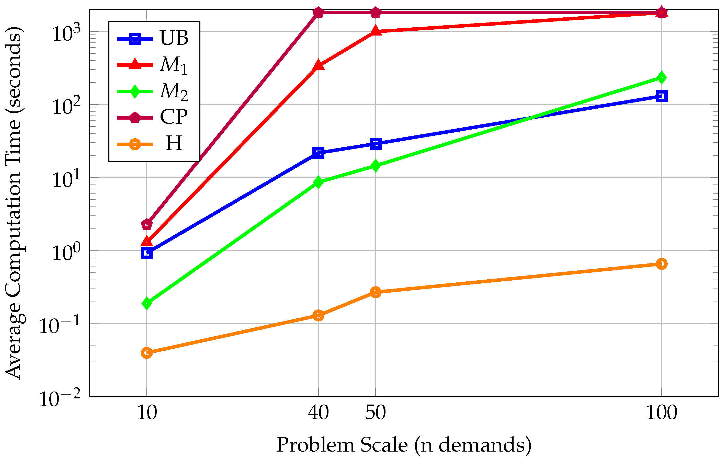
Figure 1 and Figure 2 further illustrate these trends. For small-scale instances with ten demands, all the exact methods, including the enhanced models, CP, and the computed upper bound, achieve an average of 9.8 satisfied demands, confirming that these cases are relatively straightforward to solve to optimality. In contrast, the heuristic method satisfies only 6.7 demands on average, reflecting an optimality gap of approximately 30.6 percent compared to the exact methods. In terms of computational time, $M_2$ is the fastest among the exact approaches at just 0.19 s, followed by $M_1$ at 1.3 s and CP at 2.28 s. The heuristic method is the quickest overall, requiring only 0.04 s.

In medium-scale instances with forty demands, $M_1$ and $M_2$ both satisfy an average of 30.9 demands, while the CP approach achieves a slightly lower average of 29.6, corresponding to a 4.2 percent gap relative to the top-performing models. The heuristic’s performance deteriorates more substantially at this scale, achieving an average of 22.1 satisfied demands and showing a gap of about 28.5 percent. For these instances, $M_2$ again demonstrates strong computational efficiency, solving in 8.63 s on average, whereas $M_1$ requires over 336 s and CP reaches the imposed time limit of 1800 s. The heuristic method remains the fastest at 0.13 s.

For fifty-demand instances, $M_1$ and $M_2$ each achieve an average of 45.5 satisfied demands. CP achieves a slightly lower average of 43.9, with a gap of about 3.5 percent, while the heuristic averages 34.5 satisfied demands, resulting in an optimality gap exceeding 24 percent. The computational effort required mirrors the earlier trends: $M_2$ completes in roughly 14.5 s on average, compared to 992 s for $M_1$ and the full 1800 s for CP. The heuristic remains the fastest, requiring just 0.27 s.

For the large-scale instances involving one hundred charging demands, $M_2$ achieves the highest average number of satisfied demands at 90.1, followed by CP with an average of 87.9 and $M_1$ with 83.8. Relative to the best-performing $M_2$, CP shows an inferiority gap of approximately 2.4 percent but demonstrates a modest advantage of about 4.7 percent compared to $M_1$. The heuristic method maintains its speed advantage but yields only 73.9 satisfied demands on average, which corresponds to an optimality gap of nearly 18 percent relative to the best model. In terms of computational time, $M_2$ solves these instances in around 234 s on average, while both $M_1$ and CP reach the 1800 s limit. The heuristic again produces its results almost instantaneously, at just 0.66 s.

These findings confirm the superior performance and computational efficiency of the advanced $M_2$ model for solving the preemptive EVCSP to proven optimality. Overall, these results demonstrate that the proposed models, $M_1$ and $M_2$, along with the CP approach, consistently outperform the baseline formulation of Zaidi et al. [9], which struggled to guarantee optimality even for smaller instances and relied heavily on metaheuristic methods for acceptable solutions. Nonetheless, the heuristic approach remains a reasonable choice in situations where decision speed is more critical than achieving the best possible solution quality. Moreover, while the CP approach entails higher computational costs, its strong results for small- and medium-sized instances, as well as its competitive performance relative to $M_1$ for the largest instances, highlight its potential as a viable exact alternative for tackling increasingly large and complex scheduling scenarios where a more systematic search of feasible solutions is beneficial.

9. Conclusions

This study addresses the preemptive electric vehicle charging scheduling problem (EVCSP) by developing two enhanced mathematical programming models, $M_1$ and $M_2$, alongside a constraint programming (CP) approach. These methodological contributions are designed to maximize the number of satisfied charging demands while adhering to grid capacity constraints. By refining the problem formulation and introducing an exact CP alternative, the proposed methods respond to the scalability and optimality challenges observed in earlier approaches.

The comprehensive experimental analysis demonstrates that the refined model, $M_2$, consistently achieves proven optimality across all the tested problem sizes, including large-scale scenarios, with substantially lower computational times than alternative exact methods. The results further indicate that $M_1$ achieves near-optimal solutions but generally requires more computation time, particularly for larger instances. The CP approach produces solutions that are competitive with $M_1$ and, in certain large-scale instances, even surpass its performance, although this comes with a higher computational cost. The heuristic method, while exhibiting the largest solution quality gap as the problem size increases, remains useful in contexts where computational speed is paramount and slight reductions in solution quality are acceptable. Overall, the proposed models and the CP formulation demonstrate improved solution quality and robustness compared to the baseline established in Zaidi et al. [9] and offer practical value for managing increasingly complex EV charging operations.

Future research could further enhance the CP approach by developing advanced upper-bound estimation methods and improved branching or propagation strategies to reduce computational effort on large instances. Hybrid frameworks that combine constraint programming with metaheuristic techniques or learning-based approaches, such as reinforcement learning, could also be explored to accelerate convergence while maintaining solution quality under complex real-world conditions. Incorporating stochastic programming or stochastic constraint programming would extend the models to address real-world uncertainties, including demand fluctuations, variable vehicle arrival patterns, and dynamic grid capacity. Additionally, integrating dynamic features such as vehicle-to-grid interactions and electricity price fluctuations would strengthen the models’ practical relevance for modern smart grid environments. Finally, the development of distributed or parallel solution schemes may further improve scalability, enabling real-time decision-making for geographically distributed charging infrastructures.