Article

Physics-Informed Neural Network for Nonlinear Bending Analysis of Nano-Beams: A Systematic Hyperparameter Optimization

by
Saba Sadat Mirsadeghi Esfahani
1,
Ali Fallah
2,* and
Mohammad Mohammadi Aghdam
1,*
1
Mechanical Engineering Department, Amirkabir University of Technology, Tehran 15875-4413, Iran
2
Department of Automotive Engineering, Atilim University, Ankara 06830, Turkey
*
Authors to whom correspondence should be addressed.
Math. Comput. Appl. 2025, 30(4), 72; https://doi.org/10.3390/mca30040072
Submission received: 27 April 2025 / Revised: 4 July 2025 / Accepted: 11 July 2025 / Published: 14 July 2025
(This article belongs to the Special Issue Advances in Computational and Applied Mechanics (SACAM))

Abstract

This paper investigates the nonlinear bending analysis of nano-beams using the physics-informed neural network (PINN) method. The nonlinear governing equations for the bending of size-dependent nano-beams are derived from Hamilton’s principle, incorporating nonlocal strain gradient theory, and based on Euler–Bernoulli beam theory. In the PINN method, the solution is approximated by a deep neural network, with network parameters determined by minimizing a loss function that consists of the governing equation and boundary conditions. Despite numerous reports demonstrating the applicability of the PINN method for solving various engineering problems, tuning the network hyperparameters remains challenging. In this study, a systematic approach is employed to fine-tune the hyperparameters using hyperparameter optimization (HPO) via Gaussian process-based Bayesian optimization. Comparison of the PINN results with available reference solutions shows that the PINN, with the optimized parameters, produces results with high accuracy. Finally, the impacts of boundary conditions, different loads, and the influence of nonlocal strain gradient parameters on the bending behavior of nano-beams are investigated.

1. Introduction

Advanced developments in micro-manufacturing, semiconductor processing, sensors, and actuators have facilitated a revolutionary approach to the creation of novel technologies, including Micro-Electro-Mechanical Systems (MEMSs) and Nano-Electro-Mechanical Systems (NEMSs), smart structures, and others [1]. MEMS/NEMS devices are of significant importance in a number of fields due to their advantageous characteristics, including their small size, low weight, low consumption of energy, rapid response, and proper performance, which are useful in high-precision applications. The versatility of this technology is evidenced by its extensive range of applications in many cases which highlight the significance of understanding their mechanical performance such as their static and dynamic behaviors. The impact of size-dependency on mechanical behavior in micro/nano systems is notable, as it requires that the stress field at a specific point is affected by both local and global strains.
In this case, traditional continuum mechanics are no longer sufficient since they assume the response at a point of material depends on the variables of that point, although when it comes to small size-dependent materials, the local theory breaks down. Different theories such as nonlocal elasticity theory and strain gradient theory have been developed to compensate for the limitations of classical theories. However, each has significant shortcomings that limit their application by accurately modeling small-scale materials. Nonlocal theory considers long-range interactions by making stress at a point dependent on strains in surrounding regions [2]. However, it fails to explicitly account for the material microstructure, often over-smooths stress–strain distributions, and relies on a single length scale, limiting its ability to capture complex size-dependent behaviors [3,4]. On the other hand, strain gradient theory incorporates higher-order strain derivatives to model microstructural effects and size dependency, but it assumes purely local interactions, is overly sensitive to boundary conditions, and introduces material parameters that are challenging to calibrate experimentally [5,6]. To address these limitations, nonlocal strain gradient (NSG) theory was developed, combining the strengths of both approaches. By integrating the microstructural considerations of strain gradient theory with the long-range interactions of nonlocal theory, it provides a more comprehensive framework. This hybrid model accounts for multiple length scales, and enhances predictive accuracy, making it a powerful tool for studying size-dependent phenomena in advanced materials and structures.
Determining the mechanical behavior of structures, such as their bending, vibration, and buckling characteristics, at micro- and nanoscales has consistently been an appealing topic due to the increasing need to accurately model and predict the behaviors of materials and structures in advanced engineering applications. Numerous studies in the literature have employed NSG theory to analyze these behaviors. For instance, bending behavior has been investigated in [7,8,9,10], while vibration and buckling analyses of nano-beams and nano-plates have been explored in [4,11,12]. These studies highlight the effectiveness of the combination of nonlocal strain gradient theory in capturing size-dependent phenomena at small scales. The above-mentioned literature is limited to linear analysis while in many applications the microstructures need to be highly deformed, which makes the behavior of the structure completely nonlinear. In such cases, the governing differential equations are no longer linear differential equations and have some nonlinear terms, making the equations more complex. Finding an analytical solution for this type of differential equation is challenging, if not impossible. Therefore, employing an appropriate numerical technique such as Generalized Differential Quadrature (GDQ), finite element, or finite difference (FDM) methods is crucial. However, these well-known numerical methods have inherent limitations. For example, while the FDM [13] is effective for solving strong-form differential equations, it may be constrained by complex geometries, or a GDQ method, though robust, can encounter stability issues when dealing with intricate geometries [14]. There are a few studies in the literature about the nonlinear analysis of micro/nano structure based on NSG theory. For instance, Li et al. [15] studied the effect of nonlocal strain gradient parameters and the through-thickness variation in material influences on nonlinear bending and vibration of beams. Yang et al. [16] used the DQM to solve the nonlinear problem for nano-beams using nonlocal elasticity theory. Shan et al. [17] employed higher-order shear deformation beam theory with the influence of heat and nonlinear bending and vibration analyses for FG nano-beams by using a two-step perturbation method to present the equations. Similarly, Zhang et al. [18] introduced a two-step perturbation method for nano-beams with nonlocal strain gradient theory to consider the deep post-buckling and nonlinear bending. Recently, neural networks and deep learning with a data-driven approach have been employed in various applications [19,20,21,22,23] especially engineering [24,25,26,27]. In this approach, the norm of the deviation of the network prediction from the available real data is minimized to train the model parameters [28,29].
While data-driven methods have shown excellent performance on various engineering problems, they do not take into account the underlying physics and require a sufficiently large database as training data. More recently, physics-informed neural networks (PINNs) has been introduced that can take into account the physics of the problem [29,30]. The solution of PDE/ODE in PINNs is approximated by a neural network according to a universal theorem. By minimizing a loss function that includes the PDE/ODE and the corresponding boundary and initial conditions, the network parameters are obtained. So far, a PINN has been applied successfully to solve various well-known PDEs and ODEs [28,29,31,32,33]. Therefore, the success in the implementation of PINN has led the researchers to investigate this method in solid and structural mechanics. For example, Haghighat et al. [34] used a PINN to solve 2D linear elasticity problems and concluded that the PINN showed good agreement with the FEM solutions. Wu et al. [35] implemented a PINN for the elastoplasticity problem in heterogeneous media subjected to random cyclic and non-proportional loading paths. Fallah et al. [36] used a PINN to solve bending and free vibration of a 3D FGM porous beam resting on elastic foundation. Bazmara et al. [37] also utilized a PINN to investigate the nonlinear bending of 3D functionally graded beams. Kianian et al. [38] investigated the linear bending of a nano-beam on a nonlinear elastic foundation. Recently, Eshaghi et al. [39] introduced a framework, named DeepNetBeam (DNB), based on different forms of PINNs for the analysis of functionally graded (FG) porous beams. Mirsadeghi et al. [10] used a PINN to investigate the bending behavior of nano-beams made of 2D functionally graded material, and the PINN provided results with acceptable accuracy. Nopour et al. [40] employed a PINN to solve the nonlinear structural analysis for the large deformation of FG GPL plates rested on a nonlinear elastic foundation. Hu et al. [41] used a PINN for the prediction and evaluation of solid damage. The findings suggest that a PINN is suitable for solving higher-order differential equations in structural engineering and nano mechanics.
While PINNs have proven to be effective in accurately solving differential equations, enhancing their computational efficiency remains a challenge. A significant limitation lies in the sensitivity of the results to the model’s hyperparameters. Achieving reliable and accurate outcomes requires careful fine-tuning of these parameters. However, in most studies, hyperparameters are determined using trial-and-error approaches or methods like Taguchi analysis [36]. These techniques rely heavily on user experience and require meticulous experimental design to set optimization parameters and levels, potentially introducing bias into the results. This highlights the need for more systematic and robust methods to ensure reliability and accuracy in PINN implementations.
Hyperparameter optimization (HPO) offers an advanced solution to this challenge. While traditional approaches such as grid and random searches are commonly used, they suffer from inefficiency and scalability issues. For instance, a grid search is hindered by the curse of dimensionality, while a random search often leads to suboptimal configurations. To address these drawbacks, Bayesian optimization, particularly Gaussian process (GP)-based regression, provides a systematic method for tuning hyperparameters [42]. By leveraging previously evaluated configurations, Bayesian optimization predicts the most promising parameter settings, significantly improving computational efficiency and reducing bias compared to traditional methods [43,44]. Recently, Escapil-Inchauspe and Ruz [45] demonstrated the application of Bayesian optimization for HPO in solving Helmholtz problems using PINNs. Their findings confirmed the feasibility and effectiveness of this HPO approach in systematically fine-tuning PINN hyperparameters, achieving improved accuracy and reliability compared to traditional methods.
In this study, the nonlinear bending behavior of nano-beams is analyzed using the PINN method. The nonlinear governing equations are derived based on Euler–Bernoulli beam theory, while the nonlocal strain gradient theory is incorporated to capture size-dependent effects that are unique to nanostructures. The beam deflection is approximated by a deep neural network, with its architecture optimized by minimizing a loss function that integrates the governing equations and boundary conditions. Unlike previous studies, this research adopts a systematic approach for hyperparameter fine-tuning using Bayesian optimization. This method ensures the optimal configuration of the model’s parameters, enhancing prediction accuracy. The optimized PINN predictions are validated against analytical and numerical reference solutions, demonstrating excellent accuracy in capturing the nonlinear bending behavior under various loading scenarios and boundary conditions. Additionally, the study explores the effects of boundary conditions, diverse loading configurations, and nonlocal strain gradient parameters on the bending responses of nano-beams, providing valuable insights into their structural behavior.

2. Materials and Methods

2.1. Mathematical Formulation

Figure 1 shows a nano-beam with its width b, thickness h and length L. Consider the size-dependent nano-beam to be homogenous, and the effective material properties including Young’s modulus (E) and density (ρ) to be constant through the length and thickness of the beam. Cartesian coordinates (x, y, z) are considered. The moment of inertia ( I ) and cross section area ( A ) are calculated as follows:
I = b h 3 12 A = b h
The displacement field according to the Euler–Bernoulli beam theory takes the following form:
U x , z , t = u x , t z w x V x , z , t = 0 W x , z , t = w ( x , t )
Here, U ,   V ,   a n d   W are the displacement of an arbitrary point along the x, y, and z directions, respectively, and u and w are the axial and transverse displacement of a point on the center line of the beam, respectively. Based on von Kármán theory, the only non-zero strain element is [11]:
ε x x = u x + 1 2 w x 2 z 2 w x 2 ε y y = ε z z = ε x y = ε y z = ε x z = 0

2.1.1. Nonlocal Strain Gradient Theory

Lim et al. [46] stated that the stress accounts for the nonlocal elastic and the strain gradient stress field in the high-order nonlocal strain gradient theory as follows:
t i j = σ i j σ i j m ( 1 )
where the classical stress σ i j and the higher-order stress σ i j m ( 1 ) are defined as follows:
σ i j = 0 L E α 0 x , x , e 0 a ε k l x d x
σ i j m ( 1 ) = l 2 0 L E α 1 x , x , e a ε k l , m x d x
where l is the material length-scale parameter and shows the importance of the strain gradient stress field [47], e a is the nonlocal parameter, and the nonlocal kernel function α ( x , x , e a ) satisfies the conditions developed by Eringen [3]. For the sake of simplicity, Li et al. [11] suggested that instead of the integral form of Equations (5) and (6), the differential form of the equations can be used as follows:
1 e a 2 2 σ x x = E ε x x
1 e a 2 2 σ x x ( 1 ) = l 2 E ε x x ,   x
where is represented as a one-dimensional derivative: = x . Using Equations (4), (7), and (8), the total stress relation based on the nonlocal strain gradient theory can be written as follows:
1 e a 2 2 t x x = E   ε x x l 2 E ε x x

2.1.2. Governing Equations

The axial force resultant N x x and the bending moment resultant M x x can be written as the following form:
N x x = t x x A
M x x = z t x x A
Substituting ε x x and t x x from Equations (3) and (9) to Equations (10) and (11), the force resultant N x x and M x x with the help of equilibrium equations and nonlocal strain gradient theory formulation will be take the following form:
N x x = a 2 2 N x x   x 2 + A 11 u x + 1 2 A 11 w x 2 l 2 x A 11 2 u x 2 + A 11 2 w x 2 w x
M x x = a 2 2 M x x x 2 D 11 2 w x 2 l 2 x D 11 3 w x 3
where
A 11 = E z d y = E A D 11 = z 2 E z d y = E I
Using Li et al.’s [11] suggestion, by substituting virtual strain and kinetic and potential energy in Hamilton’s principle while neglecting the inertia terms, the equilibrium equation of Euler–Bernoulli can be expressed as follows:
δ u : N x x x f = 0
δ w : 2 M x x x 2 + x N x x w x = q
where q and f are the applied external distributed load in transverse and axial directions. Since the axial force f is assumed to be zero, according to Equation (15), the first derivative of the axial force resultant is zero ( N x x x = 0 ), and consequently Equation (12) can be rewritten as follows:
N x x = A 11 u x + 1 2 A 11 w x 2 l 2 x A 11 2 u x 2 + A 11 2 w x 2 w x
Combining Equations (13), (16) and (17), the governing equations of the size-dependent beams based on the nonlocal strain gradient theory is obtained as follows:
δ w : 1 a 2 2 x 2 q + A 11 x u x + 1 2 w x 2 l 2 x 2 u x 2 + 2 w x 2 w x w x + D 11 2 x 2 2 w x 2 l 2 x 3 w x 3 = 0  
It is obvious that coupling happens between the axial and transverse displacement due the existence of geometrical nonlinearities. It is known that in the bending of beams, the axial displacement and its derivatives are negligible compared to the transverse displacement [48,49,50]. Thus, it follows that only the transverse displacement and its derivatives are considered and consequently the governing equations for the nonlinear bending of a Euler–Bernoulli beam based on NSG theory can be simplified as follows:
1 a 2 2 x 2 [ q + 3 2 A 11 2 w x 2 w x 2 l 2 A 11 4 3 w x 3 2 w x 2 w x + 2 w x 2 3 + 4 w x 4 w x 2 ] D 11 4 w x 4 + l 2 D 11 6 w x 6 = 0
The bending moment resultant can be simplified as follows:
M x x = a 2 { q + 3 2 A 11 2 w x 2 w x 2 l 2 A 11 4 3 w x 3 2 w x 2 w x + 2 w x 2 3 + 4 w x 4 w x 2 } D 11 2 w x 2 + l 2 D 11 4 w x 4
For the sake of generality (using any material), the following dimensionless parameters are defined as follows:
w ¯ = w L ,   x ¯ = x L ,   τ = a L ,   ζ = l L ,   q ¯ = q L 3 D 00 m x x = M x x L D 00 ,   d 11 = D 11 D 00 = 1 ,   a 11 = A 11 L 2 D 00 = A L 2 I
where D 00 = I E . The non-dimensional form of the governing equation of the nano-beam based on the nonlocal-strain gradient theory can be written as follows:
q ¯ τ 2 2 q ¯ x ¯ 2 + ζ 2 τ 2 a 11 w ¯ x ¯ 2 + d 11 6 w ¯ x ¯ 6 + 8 τ 2 ζ 2 a 11 2 w ¯ x ¯ 2 w ¯ x ¯ 5 w ¯ x ¯ 5 + ( 13 τ 2 ζ 2 a 11 2 w ¯ x ¯ 2 2 d 11 + 14 τ 2 ζ 2 a 11 w ¯ x ¯ 3 w ¯ x ¯ 3 3 2 τ 2 a 11 w ¯ x ¯ 2 ζ 2 a 11 w ¯ x ¯ 2 ) 4 w ¯ x ¯ 4 + a 11 2 w ¯ x ¯ 2 4 ζ 2 w ¯ x ¯ 9 τ 2 w ¯ x ¯ + 18 τ 2 ζ 2 3 w ¯ x ¯ 3 3 w ¯ x ¯ 3 + 3 τ 2 + ζ 2   2 w ¯ x ¯ 2 2 + 3 2 w ¯ x ¯ 2 a 11   2 w ¯ x ¯ 2 = 0
and the dimensionless bending moment resultant can be rewritten as follows:
m x x = τ 2 { q ¯ + 3 2 a 11 2 w ¯ x ¯ 2 w ¯ x ¯ 2 ζ 2 a 11 4 3 w ¯ x ¯ 3 2 w ¯ x ¯ 2 w ¯ x ¯ + 2 w ¯ x ¯ 2 3 + 4 w ¯ x ¯ 4 w ¯ x ¯ 2 } d 11 2 w ¯ x ¯ 2 + ζ 2 d 11 4 w ¯ x ¯ 4
Utilizing the nonlocal strain gradient theory may lead to insufficiencies in conventional boundary conditions due to the higher order of differential equations. Consequently, an additional boundary condition known as the non-classical boundary condition is introduced for use in nonlocal strain gradient models as [11]:
2 w ¯ x ¯ 2 = 0
Table 1 provides other well-known conventional boundary conditions for free, simply supported, and clamped edges.

2.2. Solution Methodology

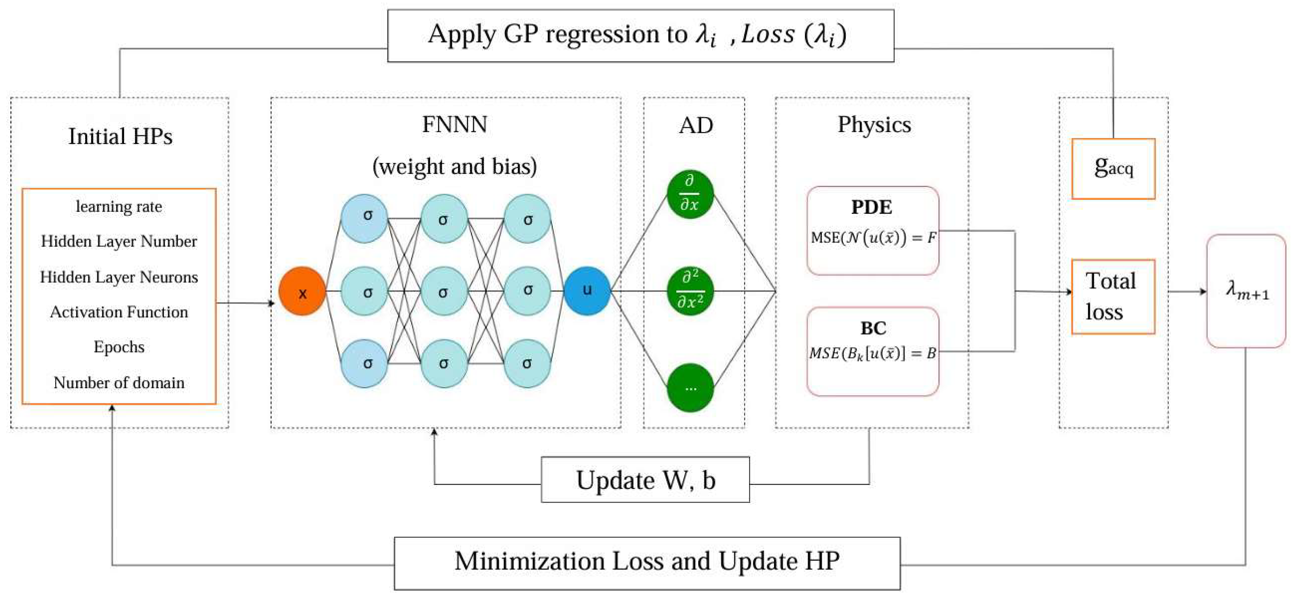
2.2.1. Physics-Informed Neural Network

In this study, the recently developed PINN, which is a mesh-free computational method, is employed for solving the governing differential equations. The PINN uses unsupervised deep learning techniques to generate solutions by training a neural network on random data points within the domain, mainly to approximate the governing ordinary or partial differential equation. It should be noted that the PINN does not need any labeled data. Raissi et al. [51] have demonstrated the effectiveness of the PINN approach in tackling nonlinear partial differential equations such as the Burgers, Schrödinger, and Allen–Cahn equations. In addition to this, results of limited available studies in the literature proved the applicability of the PINN method for the structural analysis of beams and plates [36,52,53].
The general form of the time-independent differential equation and boundary conditions on the domain can be considered as follows [36]:
D u x = D x ; u , u x 1 , , u x d ; 2 u x 1 x 1 , , 2 u x 1 x d = 0 ,       x R d
B k u x = B x ; u , u x 1 , , u x d ; 2 u x 1 x 1 , , 2 u x 1 x d = 0       o n   Ω
in which D is a linear or nonlinear differential operator, u ( x 1 , x 2 , , x d ) is the solution function to the PDE/ODE, and x i is the general framework coordinates. B k is the set of general boundary operators and Ω is the domain’s boundary which can be formed as combinations of any boundary condition such as Neumann, Dirichlet, and Mixed BCs.
According to the universal approximation theorem, any continuous function can be approximated with a feedforward neural network (FFNN) with one single hidden layer [54]. The number of neurons of that hidden layer should be increased for complicated and nonlinear functions in order to capture the whole feature of the considered function. In a deep neural network (DNN), more hidden layers with fewer neurons are employed rather than just one hidden layer with a large number of neurons [55,56]. Based on the general idea of a PINN, the unknown variable, i.e., u ( x 1 , x 2 , , x d ) , is approximated by a neural network as follows:
u x u ^ ( x ; W , b ) = N L x ; W , b : R d i n R d o u t
where N is an L layer DNN (of L 1 hidden layer) with input vector x , output vector u , and W   a n d   b are network parameters which are called the weight matrix and the bias vector, respectively. The number of neurons in the input layer, output layer, and ith hidden layer are designated as d i n , d o u t , and N n i , respectively. Various subsets of DNNs include feedforward networks, convolutional neural networks, and recurrent neural networks. Prior research has shown that feedforward neural networks (FFNNs) are effective in solving PDEs/ODEs [28]. A feedforward neural network means that it is not a loop and it is fully connected; in other words, every neuron is connected to the next one [54] and the data for each layer is derived from the preceding layer according to the nested equation employed in the feedforward neural network:
z i = σ i W i . z i 1 + b i , i = 1 , , L
At i = 0, z 0 x is the model’s input and at i = L ,   z L   u which is the model’s output. W i and b i , as mentioned previously, pertain to the weight matrix and bias vector of the ith layer, respectively. The activation function denoted by σ plays a crucial role in connecting the input and output of each layer, and various activation functions are used, such as sigmoid, sin, Swish, logistic sigmoid, Exponential Linear Unit (ELU), the hyperbolic tangent (tanh), Adaptive Piecewise Linear (APL) functions, and the rectified linear unit [28].
In the next step, the physics of the problem is incorporated by computing the derivatives of the network outputs with respect to the inputs. In the context of PINNs, the input parameters—specifically the spatial coordinates in Cartesian coordinates—carry physical implications. Consequently, differentiating the network output with respect to these input variables also carries physical implications. Unlike traditional DNNs, where derivatives pertain to network parameters such as weights and biases during training, PINNs utilize automatic differentiation (AD), also known as algorithmic differentiation, to compute derivatives with respect to input parameters. AD has been increasingly incorporated into various machine learning frameworks such as TensorFlow [57], PyTorch [58], Theano [59], and MXNet [60]. The subsequent step in PINNs involves training the network parameters by minimizing a suitable loss function that incorporates the underlying physics of the problem domain.

2.2.2. Training Procedure

The next step is training network parameters by minimizing a proper loss function that incorporates the underlying physics of the problem domain. Random training points ( x t ) including points inside the domain ( x d ) and boundary points ( x b ) are introduced. The mean square error of the total loss function (including the loss corresponding to PDE/ODE or BC ( L D and L b )) is intended to be minimized as follows:
L x t ; W , b = ω D L D x d ; W , b + ω b L b x b ; W , b
L D x d ; W , b = 1 x d x x d D x ¯ , w ¯ , w ¯ x ¯ , 2 w ¯ x ¯ , 3 w ¯ x ¯ 3 , 4 w ¯ x ¯ 4 , 5 w ¯ x ¯ 5 , 6 w ¯ x ¯ 6 2
L b x b ; W , b = 1 x b x x b B u ^ , x 2
where ω D and ω b are the weights related to domain and boundary loss functions, respectively, in which they are considered equal for simplicity. The output of the training procedure is optimized using the Adam algorithm. The whole process is illustrated in Figure 2. Since the nonlinear bending of a nano-beam is a nonlinear and concave problem, the hyperparameters must be tuned carefully to avoid random inaccurate predictions [36,61].
The algorithm of HPO via Gaussian process-based Bayesian optimization used in PINN methodology is illustrated in Figure 2, and the HPO via Gaussian process-based Bayesian optimization is explained in the further section.

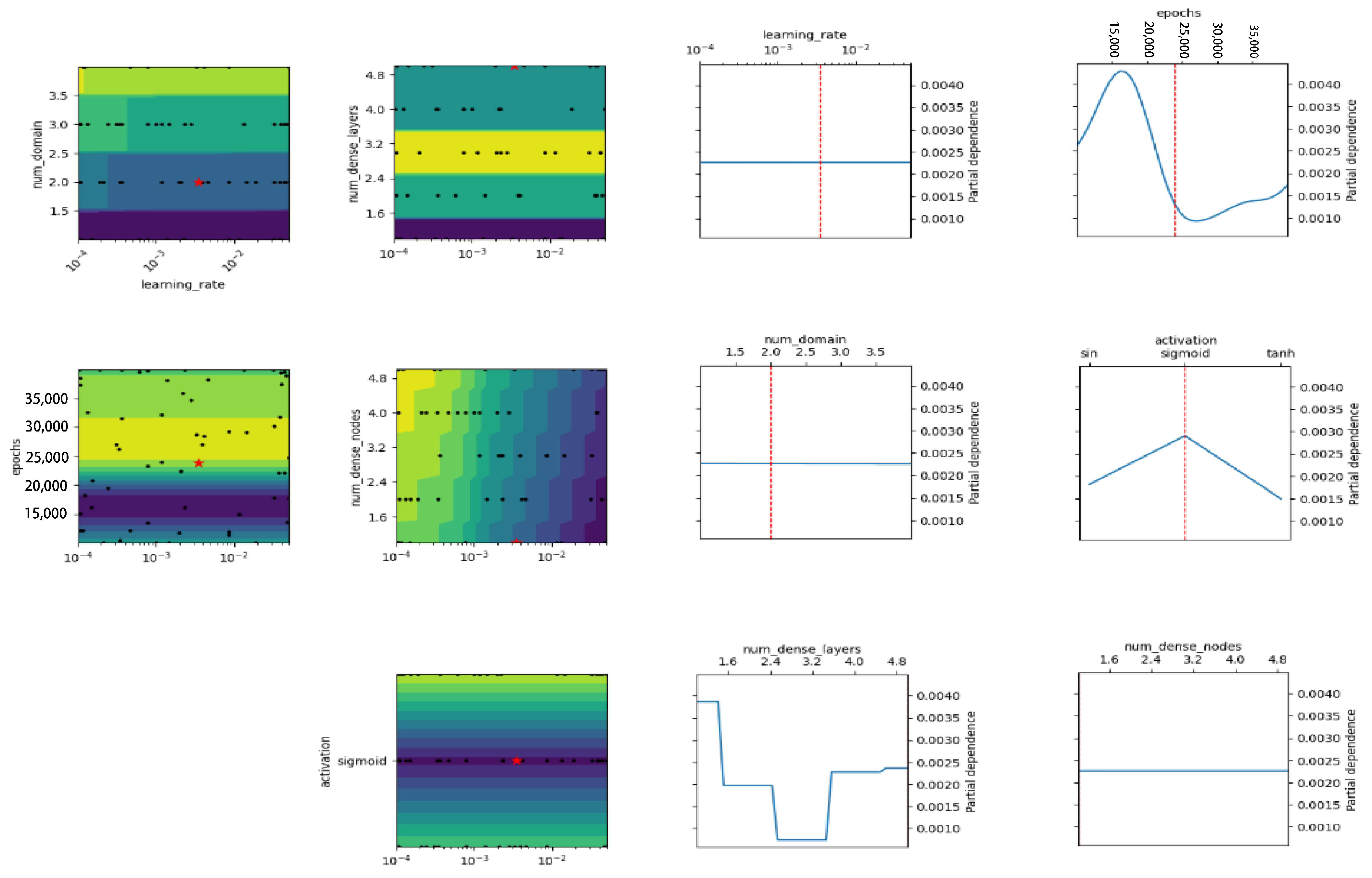
2.2.3. HPO via Gaussian Process-Based Bayesian Optimization

In the context of deep learning networks and machine learning, a hyperparameter (HP) is a kind of parameter which is set and it defines any configurable part of how a model learns. They are learned by models opposed to parameters. HPs can be either model parameters (like the activation function, or the width and hidden layer number of a NN) or algorithm parameters (like the learning rate and epochs). Some famous activation functions used in this paper for HPO are illustrated in Figure 3.
During the training process in the PINN, algorithm parameters are important for the speed of convergence. Model parameters such as the number of neurons and hidden layers measure the capacity of model learning and are determined by the complexity of function. The activation function and learning rate are considered to be categorical and logarithmical, and others are integers. λ is a set of HP configurations defined as follows:
λ = L R , N H , N n i , σ , e p o c h s , N D
where LR is the learning rate, NH is the number of hidden layers, N n i is the number of neurons in a hidden layer, σ is the activation function, and ND is the number of training points inside the domain and on the boundary.
HP tuning is the process of identifying the optimal hyperparameters, which is conducted prior to the commencement of the learning process. In the context of HPO, the goal is to identify a set of hyperparameters that will result in the lowest possible loss or the highest possible accuracy for a given objective network.
For models that are widely used, HPs can be tuned by hand and this depends on the experience of the researcher.
A manual tuning process is obtained to gain initial insights into the sensitivity of the model to different hyperparameters, which involves identifying the most significant hyperparameters, such as the number of hidden layers, the number of neurons per layer, the number of points in a domain, etc. To observe the impact on the convergence speed, training stability, and prediction accuracy (visually and through residual loss) of each hyperparameter, a range of values are individually tested through trial and error, while keeping the others fixed. This manual tuning phase was essential in defining a meaningful search space for the optimizer and ensuring the practical effective region of the hyperparameter space.
However, when attempting to solve complex problems like nonlinear bending, it is inadvisable to set the HPs manually through a trial-and-error process. Therefore, HPO is strongly recommended as a more effective approach. Unlike manual tuning, HPO automatically runs several configurations which is considered as a significant time investment, however it may take a long time to complete and often requires a powerful GPU.
HPO systematic approaches, especially on neural networks, can be classified into search algorithms (applied for sampling) and trial schedulers (early stopping method). One prevalent type of search algorithm is a sequential model-based method named Bayesian optimization (BO), designed to identify the global optimum HPs with the minimal number of trials. It represents a compromise between grid search and random search algorithms, offering a high degree of reliability.
BO uses a Bayesian probability surrogate model (prior or posterior distribution) and an acquisition function (to avoid local minimums). The probability model used in this investigation is a kind of mostly used posterior probability called GP. In BO, GP is built and then each trial is made based on the previous ones, and furthermore, GP is updated for the next trial until the most useful HP set is chosen, thus no initial knowledge of HPs is required. Further insights into HPO algorithms and BO can be found in the work of Tong et al. [44]. GP is formulated in Equation (33) where, in this equation, μ is the mean vector and k is the covariance function or kernel for random variables x i , finding the best λ as follows:
f λ G P μ λ = E x i , k λ , λ
The acquisition function employed is Expected Improvement which is defined as follows:
E I λ = E [ max f m i n y , 0 ]
Figure 4 summarizes HPO as a flowchart. The acquisition function in Equation (34) allows us to define the next point at each m (iteration) and k (epoch), respectively. The outer loop is run through M-step GP-based Bayesian HPO. For each HP, the loss function is defined as being the best ADAM epoch for k ∈ [0, K] with loss.

3. Results and Discussion

In this section, the numerical results of the nonlinear bending of the nano-beam, as predicted by the PINN, are investigated, compared, and validated with those generated by a BVP4C numerical solution in MATLAB R2019b. The dimensionless forms of equations are derived in the previous section; therefore, any isotropic material can be used. The nano-beam material is pure steel (E = 210 GPa), with dimensions of h = 100 nm, b = h, L = 20 h.
The hyperparameters of PINN is tuned by using the HPO method and the possible value range of HP configuration for the C-C and S-S boundary conditions is outlined in Table 2.
The PINN and HPO methods are implemented using DeepXDE, TensorFlow, and Scikit-Optimize. The HP configuration is initialized as λ 0 = 0.001 ,     4 ,     4 × 5 ,     t a n h ,     20,000 ,     3 × 50 . The linear bending problem is investigated for the HPO case to find the best HP values and check this with the manual tuning of HPO, and the results are added. The optimal HP configuration ( λ m ) resulting from the application of a GP-based Bayesian HPO approach to 35 calls is illustrated in Table 3.
By using the hyperparameters of Table 3, different nonlinear bending problems are solved. Loss function values range from 10 × 10−7 to 10 × 10−9 which creates high variability in the training process. The performance of HPO via GP is shown in the form of partial dependence plots which are used to visualize and analyze the interaction between the target responses of each dimension. The partial dependence plots of the objective function are represented in the next sections. Partial dependence plots estimate the relative dependence of each dimension on the loss (after averaging out all other dimensions). The performance of HPO via GP (for S-S and C-C) is shown in the following sections.

3.1. HPO via GP for Linear Bending

The comparison of linear and nonlinear bending in PINN hyperparameters has been conducted in this paper as a beneficial attempt for HPO via GP study. In this case, the linear bending of a homogenous nano-beam under a simply supported boundary condition is employed. The best hyperparameter configuration during 35 calls is λ l i n e a r _ h p o = 0.0499 ,     4 ,     1 × 5 ,     s i g m o i d ,     269,061 ,     1 × 50 and the optimum loss value is 3.7140   ×   10 7 . The best configuration during manual tuning is λ l i n e a r _ m = 0.001 ,     3 ,   15 ,     t a n h ,     20,000 ,     50 with the loss value of 10 × 10−4. For HPO via GP during an optimization process, the algorithm finds the best configuration for the lowest loss function value; however, in manual tuning, finding the optimal HP is based on experience and trial and error. The results of both manual and HPO methods are close and accurate. Figure 5 shows the best configuration of HPs and partial dependence plot for each HP in which the red stars indicate the optimal HPs and the black points show the results of the rest of the calls.
Figure 6 shows the convergence plot for this problem, illustrating the minimized test loss function versus the number of 35 iterations (denoted as m in the flowchart, shown in Figure 4). The convergence plot demonstrates the progress of the HPO used to tune the parameters of the PINN. The plot indicates that the optimizer has reached a minimum and exhibits a downward trend, signifying a reduction in the test loss function and the identification of the optimal HPs.
Figure 7 demonstrates that tuning the hyperparameters through optimization has resulted in a decreased loss function value. It shows that HPO is a reliable automatic method to optimize the hyperparameters for a PINN. Therefore, the HPO method is used for a nonlinear bending subject.

3.2. HPO via GP for S-S for Nonlinear Bending

According to Equation (3) the S-S boundary condition (BC) satisfies the moment and deflection, and for nano-beams the non-classical BC must be satisfied as well. The nonlinear bending of a nano-beam with ( τ = 0.005 ,   ξ = 0.05 ,   q ¯ = 10 ) these specifications is investigated. Figure 8 shows the partial dependence plots of the number of domains, the learning rate, the number of hidden layers, and the number of neurons as ND = 100, NH = 4, Nni = 15, and L R = 0.0022 . The optimal activation function and number of epochs are suggested as “tanh” and 260988, respectively. The optimal HP configuration is λ m _ s s = 0.00220 , 4 , 15 , t a n h , 260,988 , 2 × 50 with 10 × 10−9 loss during 35 calls.
Red stars and black points illustrated in Figure 8 are the optimal HPs and the sampling points during the HPO process, respectively. The convergence plot in Figure 9 shows a reduction in the test loss as the number of calls (or iterations) increases. Therefore, the HPO process effectively minimizes the loss function.

3.3. HPO via GP for C-C for Nonlinear Bending

The optimal HP configuration and the partial dependence plot for the nonlinear bending of a nano-beam ( τ = 0.005 ,   ξ = 0.05 ,   q ¯ = 10 ) are illustrated in Figure 10 as NH = 5, Nni = 2 × 5, and L R = 0.0034 . The activation function which gives the best loss is “tanh”. The total best configuration is λ m _ c c = 0.004997 ,   5 ,   2 × 5 ,   t a n h ,   181,619 ,   4 × 50 with 10 × 10−7 loss during 35 calls.
The best epoch and number of domains are suggested as 181,619 and 4 × 50 in the corresponding partial dependence plots which are shown in Figure 10. The convergence plot of 35 calls is illustrated in Figure 11 and shows the decrease in test loss.

3.4. PINN Results for HPO Hyperparameters

The results for different cases are studied in the following section by using the best configurations of HPO (Table 3). Figure 12 shows the effect of strain gradient (ζ) parameters on beam deflection; PINN results are compared to BVP4C MATLAB R2019b results for validation and accuracy.
Figure 13a,b show the test and train loss versus epochs for both cases of C-C and S-S boundary conditions under s uniform load. Figure 13a is noisy after 50,000 epochs. Both conditions converge well at an average loss value of almost 10 × 10−6.
Figure 14 shows the comparison of linear and nonlinear bending deflections of a nano-beam under a sinusoidal load for the S-S boundary condition. The nonlinear dimensionless bending deflection is smaller than the linear deflection since the geometric nonlinearity causes a stiffening effect that leads to lower deflections, and it can also be implied from Equation (22) that the existence of nonlinear terms increases the stiffness of the structure, and therefore the deflection decreases. Also the results of PINN prediction for linear and nonlinear is compared with BVP4C.
Figure 15 shows the effect of nonlocal strain gradient parameters on maximum beam deflection under the same sinusoidal load for different boundary conditions. As the dimensionless strain gradient parameter increases, the beam deflection decreases. Nonlocality mostly affects external load rather than beam deflection according to Li et al. [11].
Figure 16 illustrates the effect of a dimensionless external distributed load ( q ¯ ) in the transverse direction. Similarly to linear bending, as expected, by applying greater loads to the nano-beam, higher nonlinear bending deflections are obtained. Fifteen-times the load causes almost four-times the amount of deflection.

4. Conclusions

In this paper, we applied HPO via Gaussian process-based Bayesian optimization to improve the training process of PINNs. We focused on forward problems for the nonlinear bending behavior of a homogenous nano-beam using nonlocal strain gradient theory. Various problems were performed. The governing equations were derived using Hamilton’s principle and nonlocal strain gradient theory. The strain gradient and nonlocal parameters are included to explain the importance of the strain gradient stress field and the effect of the nonlocal elastic stress field on deformation.
The governing equation, a high-order nonlinear differential equation, is solved using the PINN method. In this approach, universal neural network approximation is used for the beam deflection and the network parameters were optimized by HPO via GB to decrease the high computation time of manually tuning, and HPO is suggested for complex problems. The loss function associated with the governing physical differential equation and boundary condition is minimized.
Furthermore, the effects of various parameters such as boundary conditions, loading scenarios, length-scale parameters, and the nonlocal parameter on the bending behavior of the nano-beam are investigated. The nonlinear dimensionless bending deflection is smaller than the linear deflection due to the stiffening effect introduced by geometric nonlinearity. The most important results are as follows:
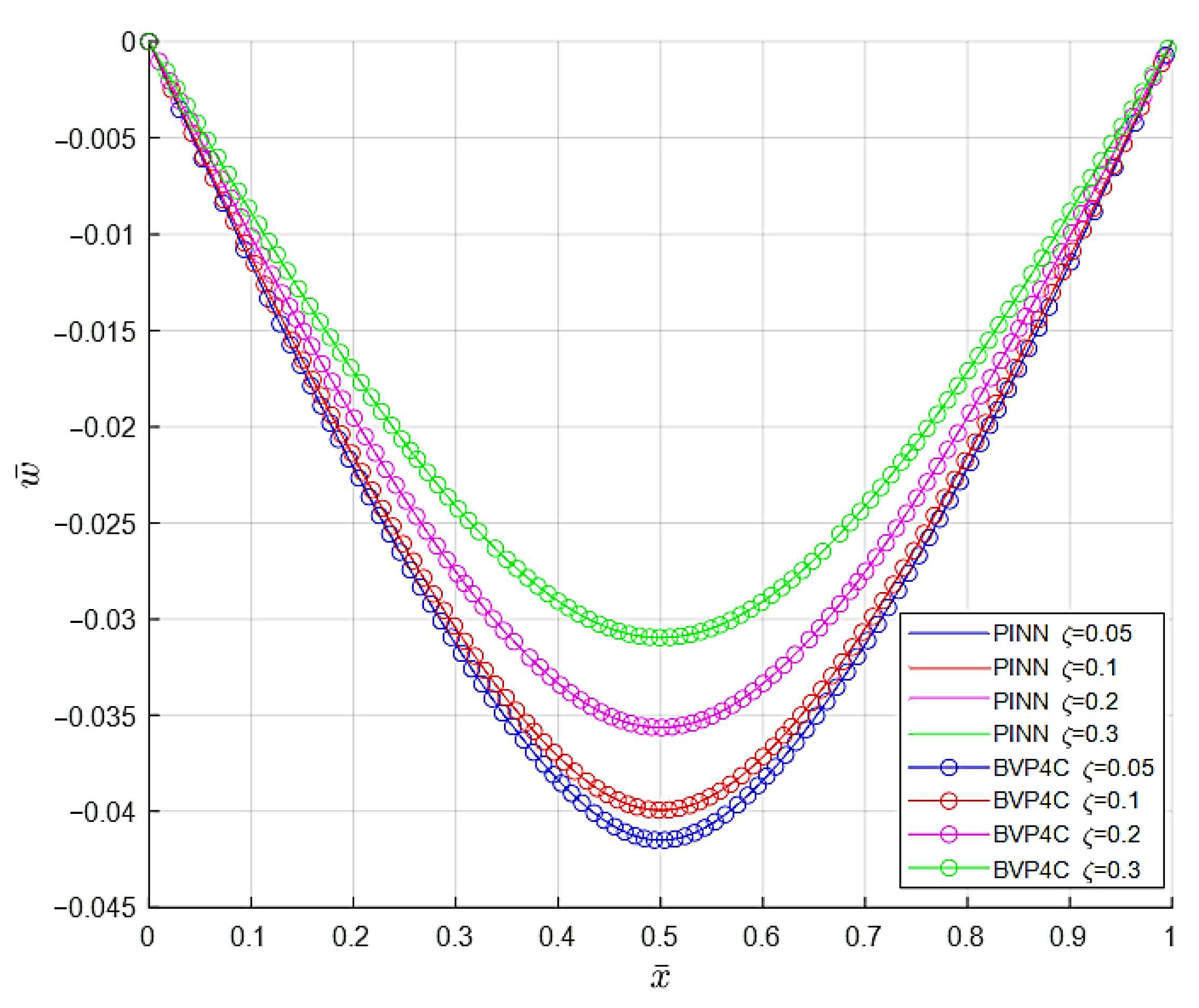
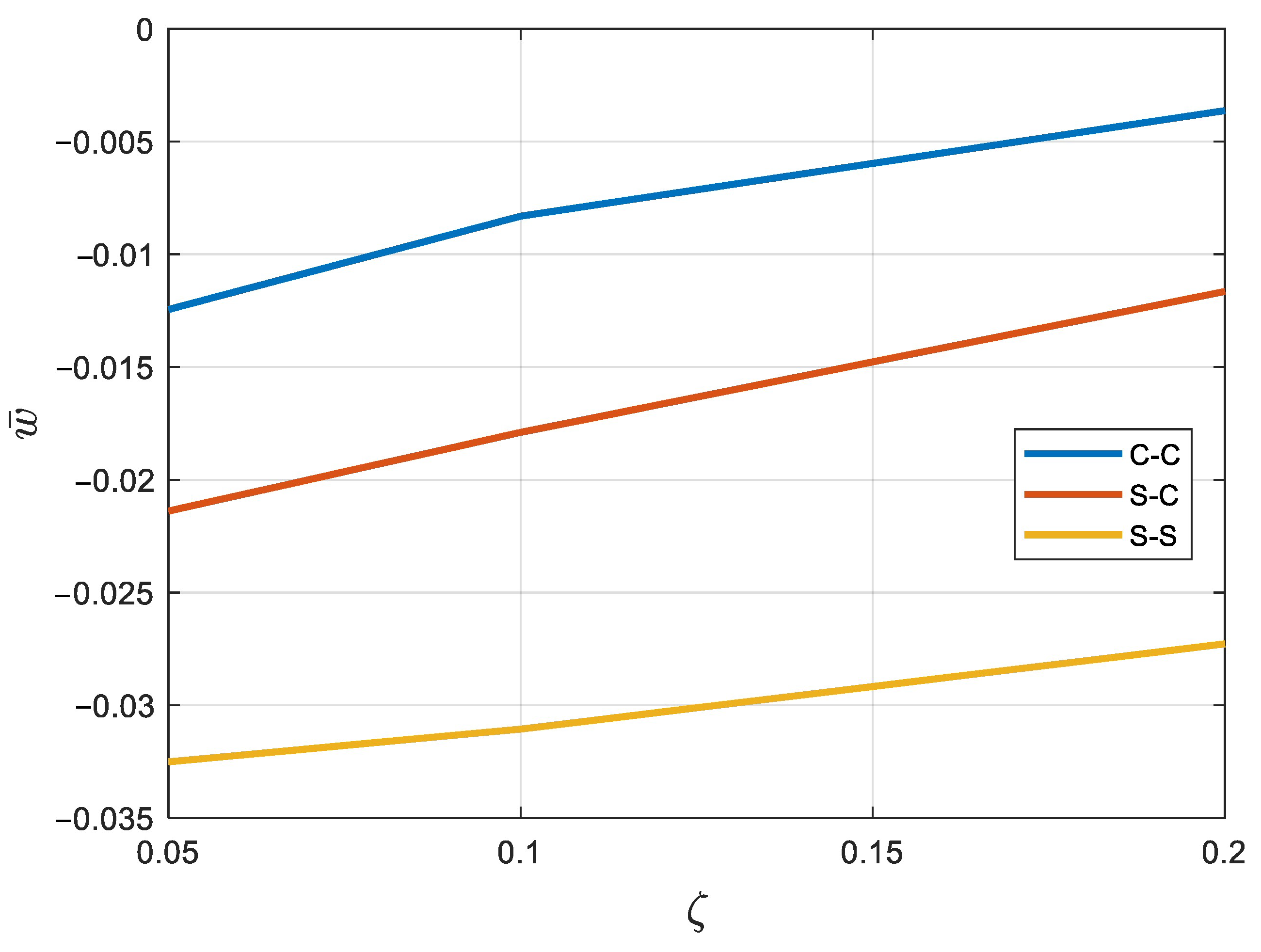
  • The results indicate that when the dimensionless strain gradient parameter is elevated, the beam displays decreased deflection. Physically, a higher nonlocal parameter implies that each material point is influenced by a larger neighborhood, effectively increasing the material’s resistance to deformation. As a result, the beam exhibits higher stiffness and consequently lower deflection under the same loading conditions.
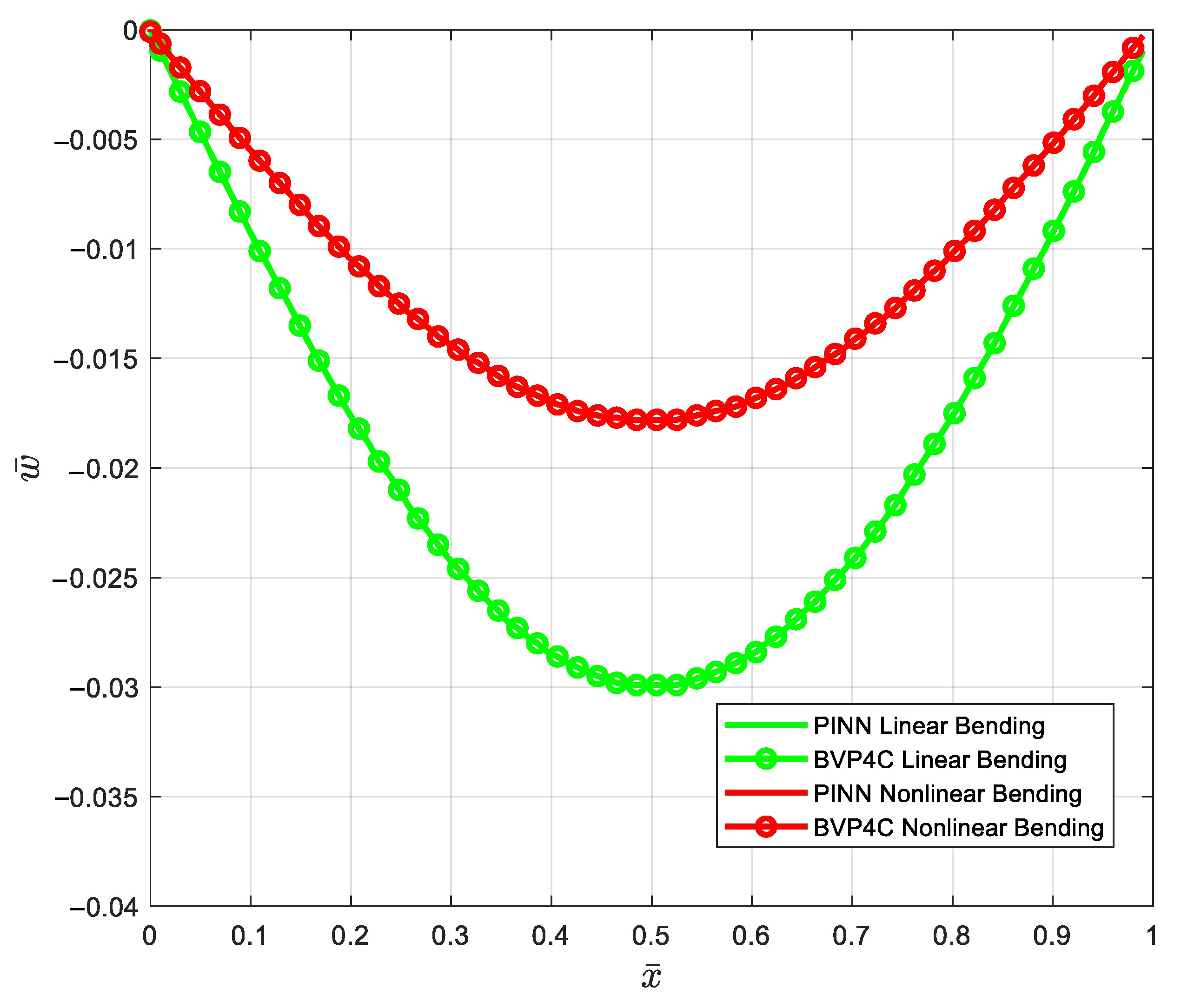
  • Due to the geometric nonlinearity which causes a stiffening effect, the nonlinear dimensionless bending deflection is smaller than the linear deflection.
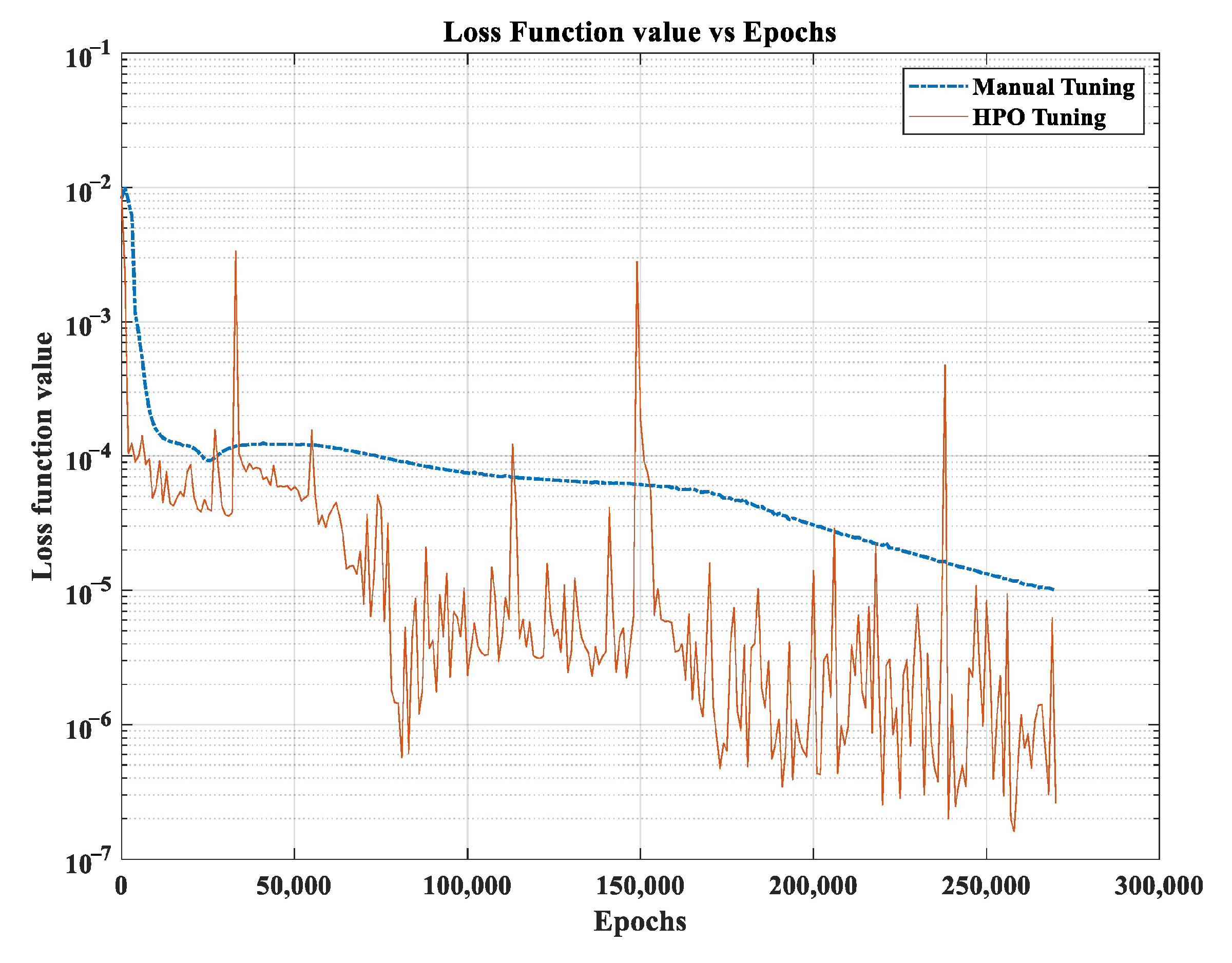
  • HPO via GP can decrease the loss function in order to tune the hyperparameters, and the results are more reliable than manually tuning mostly for complicated problems.
  • Although the HPO–GP method demonstrates great performance in finding the optimal HPs, decreasing the loss function, and improving accuracy, it comes with a high computational cost limitation, especially when applied to a large number of HPs or complex models.
The findings confirm the applicability and accuracy of the PINN method in solving higher-order nonlinear differential equations, which are considered to be a complex class of differential equations.

Author Contributions

Conceptualization, A.F.; methodology, A.F.; software, S.S.M.E.; validation, A.F. and M.M.A.; investigation, A.F. and S.S.M.E.; writing—original draft preparation, S.S.M.E.; writing—review and editing, A.F. and M.M.A.; supervision, A.F. and M.M.A. All authors have read and agreed to the published version of the manuscript.

Funding

This research received no external funding.

Data Availability Statement

All the used data have been included in the text.

Conflicts of Interest

The authors declare no conflicts of interest.

Abbreviations

The following abbreviations are used in this manuscript:
PINNPhysics-Informed Neural Network
NNNeural Network
HPHyperparameter
HPOHyperparameter Optimization
GPGaussian processes
BOBayesian Optimization

References

  1. Chuang, T.-J.; Anderson, P.; Wu, M.-K.; Hsieh, S. Nanomechanics of Materials and Structures; Springer: Berlin/Heidelberg, Germany, 2006. [Google Scholar]
  2. Reddy, J. Nonlocal theories for bending, buckling and vibration of beams. Int. J. Eng. Sci. 2007, 45, 288–307. [Google Scholar] [CrossRef]
  3. Eringen, A.C. On differential equations of nonlocal elasticity and solutions of screw dislocation and surface waves. J. Appl. Phys. 1983, 54, 4703–4710. [Google Scholar] [CrossRef]
  4. Tang, F.; He, S.; Shi, S.; Xue, S.; Dong, F.; Liu, S. Analysis of size-dependent linear static bending, buckling, and free vibration based on a modified couple stress theory. Materials 2022, 15, 7583. [Google Scholar] [CrossRef] [PubMed]
  5. Fleck, N.; Hutchinson, J. A reformulation of strain gradient plasticity. J. Mech. Phys. Solids 2001, 49, 2245–2271. [Google Scholar] [CrossRef]
  6. Gao, H.; Huang, Y.; Nix, W.D.; Hutchinson, J. Mechanism-based strain gradient plasticity—I. Theory. J. Mech. Phys. Solids 1999, 47, 1239–1263. [Google Scholar] [CrossRef]
  7. Bessaim, A.; Houari, M.S.A.; Bezzina, S.; Merdji, A.; Daikh, A.A.; Belarbi, M.-O.; Tounsi, A. Nonlocal strain gradient theory for bending analysis of 2D functionally graded nanobeams. Struct. Eng. Mech. Int’l J. 2023, 86, 731–738. [Google Scholar]
  8. Nejad, M.Z.; Hadi, A. Non-local analysis of free vibration of bi-directional functionally graded Euler–Bernoulli nano-beams. Int. J. Eng. Sci. 2016, 105, 1–11. [Google Scholar] [CrossRef]
  9. Reddy, J. Nonlocal nonlinear formulations for bending of classical and shear deformation theories of beams and plates. Int. J. Eng. Sci. 2010, 48, 1507–1518. [Google Scholar] [CrossRef]
  10. Mirsadeghi Esfahani, S.S.; Fallah, A.; Mohammadi Aghdam, M. Physics-informed neural network for bending analysis of two-dimensional functionally graded nano-beams based on nonlocal strain gradient theory. J. Comput. Appl. Mech. 2025, 56, 222–248. [Google Scholar]
  11. Li, X.; Li, L.; Hu, Y.; Ding, Z.; Deng, W. Bending, buckling and vibration of axially functionally graded beams based on nonlocal strain gradient theory. Compos. Struct. 2017, 165, 250–265. [Google Scholar] [CrossRef]
  12. Hadji, L.; Fallah, A.; Aghdam, M.M. Influence of the distribution pattern of porosity on the free vibration of functionally graded plates. Struct. Eng. Mech. Int’l J. 2022, 82, 151–161. [Google Scholar]
  13. Thomas, J.W. Numerical Solution of Partial Differential Equations: Finite Difference Methods; Oxford University Press: Oxford, UK, 1995. [Google Scholar]
  14. Marzani, A.; Tornabene, F.; Viola, E. Nonconservative stability problems via generalized differential quadrature method. J. Sound Vib. 2008, 315, 176–196. [Google Scholar] [CrossRef]
  15. Li, L.; Hu, Y. Nonlinear bending and free vibration analyses of nonlocal strain gradient beams made of functionally graded material. Int. J. Eng. Sci. 2016, 107, 77–97. [Google Scholar] [CrossRef]
  16. Yang, T.; Tang, Y.; Li, Q.; Yang, X.-D. Nonlinear bending, buckling and vibration of bi-directional functionally graded nanobeams. Compos. Struct. 2018, 204, 313–319. [Google Scholar] [CrossRef]
  17. Shan, W.; Li, B.; Qin, S.; Mo, H. Nonlinear bending and vibration analyses of FG nanobeams considering thermal effects. Mater. Res. Express 2020, 7, 125007. [Google Scholar] [CrossRef]
  18. Zhang, B.; Shen, H.; Liu, J.; Wang, Y.; Zhang, Y. Deep postbuckling and nonlinear bending behaviors of nanobeams with nonlocal and strain gradient effects. Appl. Math. Mech. 2019, 40, 515–548. [Google Scholar] [CrossRef]
  19. Abbaspour-Gilandeh, Y.; Molaee, A.; Sabzi, S.; Nabipur, N.; Shamshirband, S.; Mosavi, A. A combined method of image processing and artificial neural network for the identification of 13 Iranian rice cultivars. Agronomy 2020, 10, 117. [Google Scholar] [CrossRef]
  20. Azarmdel, H.; Jahanbakhshi, A.; Mohtasebi, S.S.; Muñoz, A.R. Evaluation of image processing technique as an expert system in mulberry fruit grading based on ripeness level using artificial neural networks (ANNs) and support vector machine (SVM). Postharvest Biol. Technol. 2020, 166, 111201. [Google Scholar] [CrossRef]
  21. Brown, B.P.; Mendenhall, J.; Geanes, A.R.; Meiler, J. General Purpose Structure-Based drug discovery neural network score functions with human-interpretable pharmacophore maps. J. Chem. Inf. Model. 2021, 61, 603–620. [Google Scholar] [CrossRef]
  22. Mignan, A.; Broccardo, M. Neural network applications in earthquake prediction (1994–2019): Meta-analytic and statistical insights on their limitations. Seismol. Res. Lett. 2020, 91, 2330–2342. [Google Scholar] [CrossRef]
  23. Le Glaz, A.; Haralambous, Y.; Kim-Dufor, D.-H.; Lenca, P.; Billot, R.; Ryan, T.C.; Marsh, J.; Devylder, J.; Walter, M.; Berrouiguet, S. Machine learning and natural language processing in mental health: Systematic review. J. Med. Internet Res. 2021, 23, e15708. [Google Scholar] [CrossRef] [PubMed]
  24. Brunton, S.L.; Kutz, J.N. Methods for data-driven multiscale model discovery for materials. J. Phys. Mater. 2019, 2, 044002. [Google Scholar] [CrossRef]
  25. Brunton, S.L.; Noack, B.R.; Koumoutsakos, P. Machine learning for fluid mechanics. Annu. Rev. Fluid Mech. 2020, 52, 477–508. [Google Scholar] [CrossRef]
  26. Yaghoubi, V.; Cheng, L.; Van Paepegem, W.; Kersemans, M. CNN-DST: Ensemble deep learning based on Dempster-Shafer theory for vibration-based fault recognition. arXiv 2021, arXiv:2110.07191. [Google Scholar] [CrossRef]
  27. Yaghoubi, V.; Cheng, L.; Van Paepegem, W.; Kersemans, M. An ensemble classifier for vibration-based quality monitoring. Mech. Syst. Signal Process. 2022, 165, 108341. [Google Scholar] [CrossRef]
  28. Lu, L.; Meng, X.; Mao, Z.; Karniadakis, G.E. DeepXDE: A deep learning library for solving differential equations. SIAM Rev. 2021, 63, 208–228. [Google Scholar] [CrossRef]
  29. Raissi, M.; Perdikaris, P.; Karniadakis, G.E. Physics-informed neural networks: A deep learning framework for solving forward and inverse problems involving nonlinear partial differential equations. J. Comput. Phys. 2019, 378, 686–707. [Google Scholar] [CrossRef]
  30. Zhu, Y.; Zabaras, N.; Koutsourelakis, P.-S.; Perdikaris, P. Physics-constrained deep learning for high-dimensional surrogate modeling and uncertainty quantification without labeled data. J. Comput. Phys. 2019, 394, 56–81. [Google Scholar] [CrossRef]
  31. Zhao, H.; Storey, B.D.; Braatz, R.D.; Bazant, M.Z. Learning the physics of pattern formation from images. Phys. Rev. Lett. 2020, 124, 060201. [Google Scholar] [CrossRef]
  32. Khalid, S.; Yazdani, M.H.; Azad, M.M.; Elahi, M.U.; Raouf, I.; Kim, H.S. Advancements in Physics-Informed Neural Networks for Laminated Composites: A Comprehensive Review. Mathematics 2024, 13, 17. [Google Scholar] [CrossRef]
  33. Fallah, A.; Aghdam, M.M. Physics-Informed Neural Network for Solution of Nonlinear Differential Equations. In Nonlinear Approaches in Engineering Application: Automotive Engineering Problems; Jazar, R.N., Dai, L., Eds.; Springer Nature: Cham, Switzerland, 2024; pp. 163–178. [Google Scholar]
  34. Haghighat, E.; Raissi, M.; Moure, A.; Gomez, H.; Juanes, R. A physics-informed deep learning framework for inversion and surrogate modeling in solid mechanics. Comput. Methods Appl. Mech. Eng. 2021, 379, 113741. [Google Scholar] [CrossRef]
  35. Wu, L.; Kilingar, N.G.; Noels, L. A recurrent neural network-accelerated multi-scale model for elasto-plastic heterogeneous materials subjected to random cyclic and non-proportional loading paths. Comput. Methods Appl. Mech. Eng. 2020, 369, 113234. [Google Scholar] [CrossRef]
  36. Fallah, A.; Aghdam, M.M. Physics-informed neural network for bending and free vibration analysis of three-dimensional functionally graded porous beam resting on elastic foundation. Eng. Comput. 2023, 40, 437–454. [Google Scholar] [CrossRef]
  37. Bazmara, M.; Silani, M.; Mianroodi, M. Physics-informed neural networks for nonlinear bending of 3D functionally graded beam. Structures 2023, 49, 152–162. [Google Scholar] [CrossRef]
  38. Kianian, O.; Sarrami, S.; Movahedian, B.; Azhari, M. PINN-based forward and inverse bending analysis of nanobeams on a three-parameter nonlinear elastic foundation including hardening and softening effect using nonlocal elasticity theory. Eng. Comput. 2024, 41, 71–97. [Google Scholar] [CrossRef]
  39. Eshaghi, M.S.; Bamdad, M.; Anitescu, C.; Wang, Y.; Zhuang, X.; Rabczuk, T. Applications of scientific machine learning for the analysis of functionally graded porous beams. Neurocomputing 2025, 619, 129119. [Google Scholar] [CrossRef]
  40. Nopour, R.; Fallah, A.; Aghdam, M.M. Large deflection analysis of functionally graded reinforced sandwich beams with auxetic core using physics-informed neural network. Mech. Based Des. Struct. Mach. 2025, 53, 5264–5288. [Google Scholar] [CrossRef]
  41. Hu, H.; Qi, L.; Chao, X. Physics-informed Neural Networks (PINN) for computational solid mechanics: Numerical frameworks and applications. Thin-Walled Struct. 2024, 205, 112495. [Google Scholar] [CrossRef]
  42. Snoek, J.; Larochelle, H.; Adams, R.P. Practical bayesian optimization of machine learning algorithms. In Proceedings of the Advances in Neural Information Processing Systems 25 (NIPS 2012), Lake Tahoe, CA, USA, 3–8 December 2012. [Google Scholar]
  43. Bergstra, J.; Bardenet, R.; Bengio, Y.; Kégl, B. Algorithms for hyper-parameter optimization. In Proceedings of the Advances in Neural Information Processing Systems 24 (NIPS 2011), Granada, Spain, 12–17 December 2011. [Google Scholar]
  44. Yu, T.; Zhu, H. Hyper-parameter optimization: A review of algorithms and applications. arXiv 2020, arXiv:2003.05689. [Google Scholar]
  45. Escapil-Inchauspé, P.; Ruz, G.A. Hyper-parameter tuning of physics-informed neural networks: Application to Helmholtz problems. Neurocomputing 2023, 561, 126826. [Google Scholar] [CrossRef]
  46. Lim, C.; Zhang, G.; Reddy, J. A higher-order nonlocal elasticity and strain gradient theory and its applications in wave propagation. J. Mech. Phys. Solids 2015, 78, 298–313. [Google Scholar] [CrossRef]
  47. Polyzos, D.; Fotiadis, D. Derivation of Mindlin’s first and second strain gradient elastic theory via simple lattice and continuum models. Int. J. Solids Struct. 2012, 49, 470–480. [Google Scholar] [CrossRef]
  48. Jang, T. A general method for analyzing moderately large deflections of a non-uniform beam: An infinite Bernoulli–Euler–von Kármán beam on a nonlinear elastic foundation. Acta Mech. 2014, 225, 1967–1984. [Google Scholar] [CrossRef]
  49. Fallah, A.; Aghdam, M.M. Nonlinear free vibration and post-buckling analysis of functionally graded beams on nonlinear elastic foundation. Eur. J. Mech.—A/Solids 2011, 30, 571–583. [Google Scholar] [CrossRef]
  50. Fallah, A.; Aghdam, M.M. Thermo-mechanical buckling and nonlinear free vibration analysis of functionally graded beams on nonlinear elastic foundation. Compos. Part B Eng. 2012, 43, 1523–1530. [Google Scholar] [CrossRef]
  51. Cuomo, S.; Di Cola, V.S.; Giampaolo, F.; Rozza, G.; Raissi, M.; Piccialli, F. Scientific machine learning through physics–informed neural networks: Where we are and what’s next. J. Sci. Comput. 2022, 92, 88. [Google Scholar] [CrossRef]
  52. Bazmara, M.; Mianroodi, M.; Silani, M. Application of physics-informed neural networks for nonlinear buckling analysis of beams. Acta Mech. Sin. 2023, 39, 422438. [Google Scholar] [CrossRef]
  53. Li, W.; Bazant, M.Z.; Zhu, J. A physics-guided neural network framework for elastic plates: Comparison of governing equations-based and energy-based approaches. Comput. Methods Appl. Mech. Eng. 2021, 383, 113933. [Google Scholar] [CrossRef]
  54. Funahashi, K.-I. On the approximate realization of continuous mappings by neural networks. Neural Netw. 1989, 2, 183–192. [Google Scholar] [CrossRef]
  55. Zhuang, X.; Guo, H.; Alajlan, N.; Zhu, H.; Rabczuk, T. Deep autoencoder based energy method for the bending, vibration, and buckling analysis of Kirchhoff plates with transfer learning. Eur. J. Mech.—A/Solids 2021, 87, 104225. [Google Scholar] [CrossRef]
  56. Mhaskar, H.N.; Poggio, T. Deep vs. shallow networks: An approximation theory perspective. Anal. Appl. 2016, 14, 829–848. [Google Scholar] [CrossRef]
  57. Abadi, M.; Barham, P.; Chen, J.; Chen, Z.; Davis, A.; Dean, J.; Devin, M.; Ghemawat, S.; Irving, G.; Isard, M. Tensorflow: A system for large-scale machine learning. In Proceedings of the 12th {USENIX} Symposium on Operating Systems Design and Implementation ({OSDI} 16), Savannah, GA, USA, 2–4 November 2016. [Google Scholar]
  58. Paszke, A.; Gross, S.; Chintala, S.; Chanan, G.; Yang, E.; DeVito, Z.; Lin, Z.; Desmaison, A.; Antiga, L.; Lerer, A. Automatic differentiation in pytorch. In Proceedings of the 31st Conference on Neural Information Processing Systems (NIPS 2017), Long Beach, CA, USA, 4–9 December 2017. [Google Scholar]
  59. Bergstra, J.; Breuleux, O.; Bastien, F.; Lamblin, P.; Pascanu, R.; Desjardins, G.; Turian, J.; Warde-Farley, D.; Bengio, Y. Theano: A CPU and GPU math expression compiler. In Proceedings of the Python for Scientific Computing Conference (SciPy), Austin, TX, USA, 28 June–3 July 2010; pp. 1–7. [Google Scholar]
  60. Chen, T.; Li, M.; Li, Y.; Lin, M.; Wang, N.; Wang, M.; Xiao, T.; Xu, B.; Zhang, C.; Zhang, Z. Mxnet: A flexible and efficient machine learning library for heterogeneous distributed systems. arXiv 2015, arXiv:1512.01274. [Google Scholar]
  61. Kingma, D.P.; Ba, J. Adam: A method for stochastic optimization. arXiv 2014, arXiv:1412.6980. [Google Scholar]
Figure 1. Schematic figure of the nano-beam.
Mca 30 00072 g001
Figure 2. PINN and hyperparameter optimization algorithm.
Mca 30 00072 g002
Figure 3. The famous activation functions employed in this study for HPO.
Mca 30 00072 g003
Figure 4. Flowchart of GP-based Bayesian HPO.
Mca 30 00072 g004
Figure 5. Best HP configurations and the partial dependence plots for the linear bending of a homogenous nano-beam with the S-S boundary condition ( τ = 0.005 ,   ξ = 0.05 ,   q ¯ = 10 ) .
Mca 30 00072 g005
Figure 6. Convergence plot for the linear bending of a homogenous nano-beam with the S-S boundary condition ( τ = 0.005 ,   ξ = 0.05 ,   q ¯ = 10 ) .
Mca 30 00072 g006
Figure 7. Comparison of loss function value plot for linear bending of homogenous nano-beam with S-S boundary condition for HPO and manual HP tuning ( τ = 0.005 ,   ξ = 0.05 ,   q ¯ = 10 ) .
Mca 30 00072 g007
Figure 8. Optimal HP value and the partial dependence plot for the S-S boundary condition of the nonlinear bending of a nano-beam.
Mca 30 00072 g008
Figure 9. Convergence plot for S-S boundary condition of nonlinear bending nano-beam.
Mca 30 00072 g009
Figure 10. Optimal HP value and the partial dependence plot for the nonlinear bending of a nano-beam under the C-C boundary condition. The red stars demonstrate the optimal HPs.
Mca 30 00072 g010
Figure 11. The convergence plot for the C-C boundary condition.
Mca 30 00072 g011
Figure 12. The effect of the strain gradient parameter on the dimensionless deflection of an S-S nano-beam; the result is compared with BVP4C for validation ( q ¯ = 10 ,   τ = 0.25 ) .
Mca 30 00072 g012
Figure 13. The nonlinear bending train and test loss of the PINN method for (a) clamped–clamped (C-C) and (b) simply supported–simply supported (S-S) boundary conditions ( q ¯ = 10 ,   τ = ξ = 0.05 ) .
Mca 30 00072 g013
Figure 14. The comparison of linear and nonlinear dimensionless deflection of S-S nano-beam and validation of the PINN results via BVP4C ( q ¯ = 3 sin π x ,   τ = 0.005   ,   ξ = 0.05 ) .
Mca 30 00072 g014
Figure 15. Maximum dimensionless deflection of nano-beam for various ξ values under different boundary conditions ( q ¯ = 10 sin π x , τ = 0.2 ).
Mca 30 00072 g015
Figure 16. The effect of various values of a uniform distributed load on the nonlinear bending of a nano-beam in S-S boundary conditions ( τ = 0.005   ,   ξ = 0.05 ).
Mca 30 00072 g016
Table 1. Different types of classical boundary conditions.
Type of Boundary ConditionConstrained Items
Free edge m x x x ¯ = 0 , m x x = 0
Clamped edge w ¯ = 0 , w ¯ x ¯ = 0
Simply supported edge w ¯ = 0 ,     m x x = 0
Table 2. Overview of HPs and their possible value ranges for HPO.
HP LRNH N n i σEpochsND
Case of Study
C-C[0.0001, 0.05][1, 5] [ 1 ,   5 ]   × 5 [ t a n h ,   s i n ,   s i g m o i d ][20,000, 300,000] [ 1 ,   5 ]   × 50
S-S
Table 3. Optimal HP configuration for minimum loss of nonlinear bending of nano-beam for S-S and C-C BCs ( τ = 0.005 ,   ξ = 0.05 ,   q ¯ = 10 ) .
CaseOptimum Loss Value Best   Configuration   ( λ m )
C-C 1.48   × 10−7 λ m _ c c = 0.004997 ,       5 ,       2 × 5 ,       t a n h ,       181,619 ,       4 × 50
S-S 4.38   × 10−9 λ m _ s s = 0.002203 ,       4 ,       4 × 5 ,       t a n h ,       260,988 ,       2 × 50
Disclaimer/Publisher’s Note: The statements, opinions and data contained in all publications are solely those of the individual author(s) and contributor(s) and not of MDPI and/or the editor(s). MDPI and/or the editor(s) disclaim responsibility for any injury to people or property resulting from any ideas, methods, instructions or products referred to in the content.

