Abstract
Pharmacokinetic modelling is extensively used in understanding drug behavior, distribution and optimizing dosing regimens. This study presents a two-compartment pharmacokinetic model developed using three numerical approaches that includes the Euler method, fourth-order Runge–Kutta method, and Adams–Bashforth–Moulton method. The model incorporates key parameters including elimination, transfer rate constants, and compartment volumes. The numerical approaches are used to simulate the concentration of drug profiles, which are then compared to the exact solution. The results reveal that with an average error of 1.54%, the fourth-order Runge–Kutta technique provides optimized results compared to other methods when the overall average error is taken into account, which shows that the Runge–Kutta method is better in terms of accuracy and consistency for drug concentration estimates in the two-compartment model. This mathematical model may be used to optimize dosing procedures by providing a less complex method. Along with that, it also monitors therapeutic medication levels, which provides accurate analysis for drug distribution and elimination kinetics.
1. Introduction
The role of modern drug delivery systems in clinical pharmacology and personalized medicine is increasing with improvements in health and allied facilities [1,2]. Different mathematical techniques and methods are adopted to determine the optimized solution for solving the differential equations of different systems [3,4]. Specifically, when dealing with infectious diseases, various methods and techniques are tested in order to optimize the drug delivery process [5,6]. Pharmacokinetics is the science of the kinetics of drug absorption and disposition. These studies involve both experimental and theoretical methodologies. The subsequent methodology involves the establishment of pharmacokinetic models that aid in the estimation of drug disposition after administration [7]. Pharmacokinetic modeling plays a vital role in understanding the behavior of drugs in the human body and optimizing dosing regimens for therapeutic efficacy [8]. It provides useful insights into drug kinetics and enables the estimation of drug concentrations at different periods by measuring the mechanisms of drug absorption, distribution, metabolism, excretion, and toxicity (ADMET) [9,10]. These models are designed to apprehend the pharmacokinetics of oral, intravenous, intramuscular, subcutaneous, transdermal, topical, and inhalation routes of drug administration. These models enable easy interpretation of the volume of distribution and drug clearance, which in turn can be substantial in the calculation of the half-life of the drug [11]. This information is important for setting proper dosage levels, dosing intervals, and monitoring therapeutic medication levels in patients [12].
Pharmacokinetic models are divided into three different categories that include compartmental, non-compartmental, and physiological models [13], with the former being an extensively used model for the pharmacokinetic depiction of drugs. Among mammillary, catenary, open, and closed models of the compartmental approach, an open model for the intravascular route is described in this paper. This classification is based on the arrangement of compartments that includes a space where drugs can be distributed and eliminated, which could be in parallel or series. For capturing the dynamic interactions between drug concentrations in different parts of the body in complex pharmacokinetic systems involving numerous compartments, mathematical modeling becomes of vital importance [14]. Various studies and research have been performed in order to devise an efficient mechanism for drug delivery systems. The two-compartment model framework for representing drug distribution between a central compartment, which includes highly perfused organs, and a peripheral compartment, in which the drug distributes slowly, is discussed [15]. This model includes the drug’s transfer between compartments as well as its elimination from the system. Most medications, through an intravenous infusion, enter the systemic circulation and take a certain amount of time to distribute throughout the body. The concentration of drugs in plasma will drop more quickly during the distributive phase than it will during the post-distributive phase, which includes the complex phase, which involves interaction between drugs, tissues, and organs. In the central compartment, the concentration of the drug decreases during the distributive phase more rapidly as compared to the post-distributive phase. On the other hand, in the peripheral compartment, the drug concentration declines exponentially with respect to time [16]. The serum levels of such intravenous infusions could be estimated using this two-compartment model [17].
The pharmacokinetics of sisomicin were investigated in four healthy volunteers following intramuscular and intravenous injection [18]. The compartment model for pharmacokinetics was aligned with the elimination rate of the antibiotic, which is typified by the slow and fast disposition rate constants of 0.072 and 0.004 min−1, correspondingly [19]. For the assessment of plasma concentration after levodopa infusion as per the loading and maintenance dose protocol, the two-compartment model was employed. Blood samples were obtained for the determination of kinetic rates of levodopa as it is transported between two compartments and eliminated from the vascular space [20]. A non-standard finite difference technique was used to address the two models, which are IV infusion and IV bolus injection two-compartment pharmacokinetic models. The authenticity of the nonstandard finite difference (NSFD) method is addressed through its evaluation against other methods. It was found out that this technique provides consistent results in resolving the troubles regarding pharmacokinetic modelling [21]. Another study was conducted on human beings to investigate the ADMET of pentobarbital that was administered by extravascular and intravascular routes by employing the two-compartment open model [22]. The effectiveness of the two-compartment model is proved with the help of two tests conducted in vivo. One of them was performed to compare the different routes of administrations of trobicin, and the other was conducted on five subjects in which d-lysergic acid diethylamide was administered through IV route [23]. With the purpose of investigating the pharmacokinetics of mizolastine, which was the latest H1 antagonist, through intravenous and oral routes of administration, non-compartmental and two-compartmental models were utilized. Later, one with zero-order absorption was proven to be the optimistic approach for the analysis of the fundamental kinetics of the drug [24].
Numerical approaches are essential tools for solving differential equations that characterize pharmacokinetic models and simulating drug concentration profiles [25]. To approximate the solutions of these equations and offer estimates of drug concentrations over time, multiple numerical approaches have been developed. In this study, three widely used numerical approaches, the Euler method [26], fourth-order Runge–Kutta method [27], and Adams–Bashforth–Moulton method [28], were compared. The Euler method is a fundamental and less computational method that approximates the solution by applying the system’s derivative iteratively at each time step. Its precision, however, is restricted by its first-order approximation, which can result in major inaccuracies, especially in complicated pharmacokinetic systems [29].
The fourth-order Runge–Kutta method is a higher-order numerical method that increases accuracy by computing many intermediate stages. It outperforms the Euler method in terms of stability and precision and is commonly used in pharmacokinetic modeling [30].The Adams–Bashforth–Moulton method associates an explicit Adams–Bashforth predictor with an implicit Adams–Moulton corrector. It balances accuracy and computational efficiency and is suitable for modeling drug concentrations in complex systems [31]. In this study, we analyzed and examined the performance of numerical approaches, the Euler method, fourth-order Runge–Kutta method, and Adams–Bashforth–Moulton method, in modeling drug concentration profiles in a two-compartment pharmacokinetic system. To verify the models’ applicability to practical situations, key factors such as elimination and transfer rate constants, as well as compartment volumes, were considered [32]. The fractional differential equation model was also utilized, which accounts for local dependencies. The Caputo derivative was used to define the dynamics of the system in the fractional differential equation-based two-compartment model [33]. In other research, different methods of using the fractional differential equation related to a two-compartment model are discussed [34].
This study was conducted to evaluate the accuracy, precision, and computing efficiency of different numerical approaches by analyzing and comparing the numerical results produced using the Euler method, fourth-order Runge–Kutta method, and Adams–Bashforth–Moulton method, with a precise solution. The results of this research study will provide sensitive information that will assist in the selection of appropriate numerical and mathematical approaches for pharmacokinetic modeling. Furthermore, the findings will help to optimize dosing techniques and improve drug-concentration prediction in two-compartment systems [35].
2. Materials and Methods
2.1. Two Compartmental Pharmacokinetic Model
The two-compartment pharmacokinetic model employed in this study is a mathematical representation of how a drug operates and is delivered in the human body. The model assumes a single intravenous (IV) bolus administration, with the drug introduced directly into the central compartment at time t = 0. To effectively describe the behavior of the drugs, the model includes the following parameters. The elimination rate constants k10 and k12 represent the rates at which the drug is eliminated from the central compartment and transported from the central to the peripheral compartment, respectively. The rate at which the drug moves from the peripheral to the central compartment is represented by the transfer rate constant (k21). The unit of all the rate constants is per hour (1/h). Furthermore, compartment volumes V1 and V2 are provided to account for distribution volume (in liters) in the central and peripheral compartments, respectively. The amount of drug in each compartment is represented in Equations (1) and (2) [36],
The system of ordinary differential equations (ODEs) for the amount of drug in each compartment is given by Equations (3) and (4) [37],
Alternatively, these equations can be expressed in terms of concentrations by dividing the amount of drug by its compartment volume. A system of ordinary differential equations determines the drug concentrations in each compartment, indicated as Cc and Cp for the central and peripheral compartments (in mg/L), respectively. Equations (5) and (6), as follow, illustrate how drug concentrations fluctuate over time in the human body [38]:
These equations depict the rates of change in drug concentration in the central and peripheral compartments. The elimination, transfer, and distribution processes are taken into consideration.
In Equation (5), is the rate of change in drug concentration in the central compartment and is determined by three terms. The first term, , denotes the drug transfer from the central to the peripheral compartment. The second term, , represents the elimination process from the central compartment, where k10 represents the elimination rate constant. The negative sign specifies that the drug concentration falls over time. The third term, , signifies the drug transfer from the peripheral to the central compartment and also depicts an increase in drug concentration in the central compartment.
In Equation (6), defines the rate of change in drug concentration in the peripheral compartment and also emphasizes the dynamics of the peripheral compartment. The first term, , represents the drug transfer from the central to the peripheral compartment, and the second term, , represents the drug transfer from the peripheral to the central compartment.
These equations, together, capture the relationship between drug elimination, inter-compartmental transfer, and the resulting changes in drug concentration over time in both central and peripheral compartments. Differential equations, solved by the Euler method, fourth-order Runge–Kutta method, and Adams–Bashforth–Moulton method, are used to simulate the drug concentration and analyze the drug behavior in a two-compartment pharmacokinetic system. This provides a better understanding of the dynamics of drug distribution and elimination, and how medications are dispersed throughout the body and eliminated over time.
2.2. Numerical Methods
To simulate drug-concentration profiles and solve systems of ordinary differential equations of two-compartment models, three numerical methods were used, including the Euler method, fourth-order Runge–Kutta method, and Adams–Bashforth–Moulton method. These methods are widely utilized in finding numerical solutions for initial value problems due to their reliability and computational efficiency. Especially, the Euler method offers a simple first-order approach, the Runge–Kutta method provides higher accuracy through intermediate slope evaluations, and the Adams–Bashforth–Moulton method balances efficiency and precision in multistep integration processes.
2.2.1. Euler Method
The Euler method is a simple numerical method that is used to approximate the solution of ordinary differential equations. In this method, time interval is divided into small steps and approximating the derivative of each step based on the slope of the tangent line. The concentration of the drug at each time step is evaluated using Equations (7) and (8):
2.2.2. Fourth-Order Runge–Kutta Method
The fourth-order Runge–Kutta method is a numerical approach for solving ordinary differential equations accurately. It gives a more accurate approximation than the Euler method. This method computes multiple intermediate values to estimate the derivative at various points in the time step. The fourth-order Runge–Kutta method is used in Equations (9)–(12), as follow, to calculate the drug concentration in the central compartment at each time step.
The drug concentration in the central compartment can be simulated as in Equation (13),
For the peripheral compartment, Equations (14)–(18) can be used to evaluate the drug concentration,
The drug concentration in the peripheral compartment can be simulated as,
2.2.3. Adams–Bashforth–Moulton Method
Another numerical technique for approximating the solution of ordinary differential equations is Adams–Bashforth–Moulton method. This is a prediction correction method that combines the Adams–Bashforth prediction method and the Adams–Moulton correction method. The following procedures based on predictor and corrector steps are used to compute the drug concentration at each time step. The predictor formula approaches a solution at the next time step based on the current and previous time steps. The general form of the predictor formula equations is depicted as Equations (19) and (20):
where represent drug concentration in the central and peripheral compartments at the previous time step, and are the corresponding derivative values.
The corrector step is then performed to improve the estimations, as depicted in Equations (21) and (22),
where are the updated concentrations at the current time step; and are the predicted derivative values obtained at the predictor step.
2.3. Analytical Approach
The analytical solution of the two-compartment pharmacokinetic model provides a mathematical framework to describe the distribution and elimination of a drug within the body. This model considers the central compartment and the peripheral compartment, with drug transfer and elimination governed by first-order kinetics. The dynamics of these concentrations over time are represented by the system of Equations (1) and (2). To solve this system analytically, the system is written in matrix vector form:
where and .
The eigenvalues of matrix A are determined by solving the characteristic equation:
This leads to a quadratic equation in λ, and solving it gives two eigenvalues. These values are then used to form the general solution, which includes exponential terms based on how the system behaves over time. The direction and shape of the solution are guided by the corresponding eigenvectors. To get the final expressions, initial values of the drug concentrations are used, which are explained in the Section 3.
3. Results
To determine the analytical solution, consider the constant of the rate of drug transfer from the central compartment to the peripheral compartment as , and the elimination rate constant from the central compartment as . The transfer rate constant at which the drug moves from the peripheral compartment to the central compartment is . The initial condition of the system is considered as Then the system of equation will be represented as,
The matrix form of the system is:
The eigenvalues of matrix A can be determined by solving the equation , which leads to a quadratic equation.
The eigenvectors for each eigenvalue and are and , respectively.
The general solution of the given system is:
To find out the particular solution, it is necessary to determine the values of the constants ‘a’ and ‘b’ by applying the initial conditions,
The following two equations are obtained,
The particular solution of the given system is:
Separately, the particular solution can be written as:
To simulate drug-concentration profiles in the two-compartment pharmacokinetic model, three numerical methods (Euler, fourth-order Runge–Kutta, and Adams–Bashforth–Moulton) were used in computational software. To test the performance of each method, the simulated results were compared with the accurate solution.
The simulation results show that in the two-compartment model, the fourth-order Runge–Kutta approach consistently provided accurate estimates for drug concentrations in both compartments, as depicted in Table 1 and Table 2. The drug concentration profiles acquired using this approach were identical to the profiles obtained from the analytical solution, exhibiting minimal deviation. This shows that the fourth-order Runge–Kutta approach can accurately capture the dynamics of drug distribution and elimination in the two-compartment system, as depicted in Figure 1.

Table 1.
Drug concentrations in the central compartment.
Table 2.
Drug concentrations in the peripheral compartment.
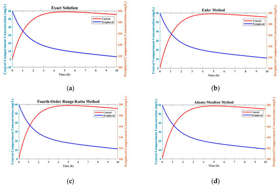
Figure 1.
Comparison of drug concentration profiles using different numerical methods: (a) exact solution; (b) Euler method; (c) fourth-order Runge–Kutta method; (d) Adams–Bashforth–Moulton method.
In Figure 1, the Euler method shows significant deviations from the exact solution, especially in the scenario with rapidly changing drug concentrations. This method was less accurate and stable compared to the fourth-order Runge–Kutta method. The greater accuracy and simplicity of the Euler method come with increasing errors and limitations in handling complex reaction kinetics and rapid changes in drug concentration. A predictor correction method, the Adams–Bashforth–Moulton method, showed intermediate performance between the Euler method and fourth-order Runge–Kutta method. It gave more accurate results than the Euler method, but still had more deviations from the exact solution than the fourth-order Runge–Kutta method.
Error Analysis
Three numerical approaches were used to determine the errors for drug concentration in the central compartment, including Euler, fourth-order Runge–Kutta, and Adams Basforth Moulton. The errors represent the difference in drug concentrations predicted by each approach, and the exact solution.
Table 3 illustrates the absolute errors for drug concentration in the central compartment at various time intervals. All three approaches demonstrate some degree of error, with the fourth-order Runge–Kutta method having the lowest error when compared to the Euler method and Adams–Basforth–Moulton method. This suggests that the fourth-order Runge–Kutta technique predicts drug concentrations more accurately in the central compartment. As the simulation progresses, the error decreases, showing that the numerical approaches converge to the exact solution over time. However, at the end of the process, there are some errors and deviation in all approaches, as shown in Figure 2.
Table 3.
Error of drug concentrations in the central compartment.
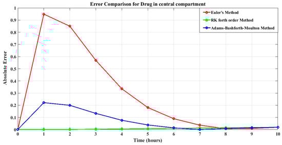
Figure 2.
Error of drug concentrations in the central compartment of all three methods.
Table 4 shows the absolute errors for drug concentration in the peripheral compartment at various time points. In terms of the best approach, a comparison of errors shows that the fourth-order Runge–Kutta method consistently produces the lowest errors among the three ways for calculating drug concentration. As a result, the fourth-order Runge–Kutta method is the most reliable and accurate solution for simulating drug concentrations and optimizing dosing techniques in this specific pharmacokinetic system, not only for the drug concentration in the central compartment but also for the drug concentration in the peripheral compartment. The errors tend to decrease as time increases, indicating convergence towards the exact solution, as shown in Figure 3.
Table 4.
Error of drug concentrations in the peripheral compartment.
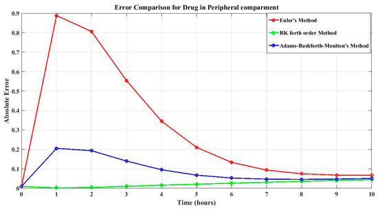
Figure 3.
Error of drug concentrations in the peripheral compartment of all three method.
Table 5 shows the average errors for the central and peripheral compartments, as well as the overall average error, calculated using three different numerical methods that include the Euler method, fourth-order Runge–Kutta method, and Adams–Bashforth–Moulton method. With an average error of 0.0154, the fourth-order Runge–Kutta method shows better results than the other methods when the overall average error is taken into account. The total average error for the Adams–Bashforth–Moulton method is 0.0766, while the overall average error for the Euler method is 0.2862.
Table 5.
Overall average of errors of drug concentrations in both compartments.
Based on these findings, the fourth-order Runge–Kutta method delivers the most correct and reliable predictions for drug concentrations in both compartments and also in the two-compartment pharmacokinetic system. The performance comparison with reference to error between these analytical methods and exact solution are depicted in Figure 4.
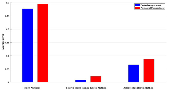
Figure 4.
Average error of drug concentrations in the central compartment of all three methods.
4. Discussion
The two-compartment pharmacokinetic model was used to evaluate the operation of drugs in the body. To estimate the process of drug function, different parameters were used in the model. The rate at which the drug was eliminated from the central compartment was k10 = 0.05 per hour, while the rate at which the drug was transported from the central to the peripheral compartment was k12 = 0.5 per hour. The transfer rate constant, k21 = 0.25 per hour, is the rate at which the drug transfers from the peripheral to the central compartment. The initial condition of the drug concentration in the central compartment at t = 0 is 0, and the drug concentration in the peripheral compartment at t = 0 is 200. By taking all these values of the different parameters, the differential equations of the model are solved analytically to get an exact solution.
Several studies have been conducted in order to determine the approximation results of the mathematical model of the drug concentration in the two-compartment model. In this study, three different numerical methods are compared with the exact solution of the two-compartment model. The simplest method to get the approximate solution of the ordinary differential equations is the Euler method. In this method, the concentration of the drug in the central compartment and peripheral compartment is calculated at each time step of 0.1. The results obtained from this method are highly deviated from the exact solution.
Another approximation method used to estimate the drug concentration is fourth-order Runge–Kutta method. This method calculates multiple intermediate values to approximate the drug concentration at each time step. For a single iteration, intermediate values have to be calculated, making it a lengthy process. But the results obtained from this method are very close to the exact solution for both compartments. One more approximation method is the Adams–Bashforth–Moulton method, which is used to calculate drug concentration in the central compartment and peripheral compartment. This method consists of two steps, predictor and corrector steps, that are based on the current and previous time steps. The values obtained from the predictor step are used in the corrector step to approximate the drug concentration of each iteration. This method gives good approximation results but still has slightly more deviations from the exact solution.
Our comparative examination of the traditional numerical methods adds to the existing researches in sophisticated modelling techniques, which include fractional-order compartmental models employing the Grünwald–Letnikov scheme to capture anomalous diffusion behavior more effectively [39]. Ref. [34] also shows that fractional-order compartmental models can better describe anomalous pharmacokinetic behavior, though with added complexity due to mass balance difficulties [34]. Recent research on nonstandard finite difference schemes shows that they are effective in solving one-compartment pharmacokinetic models for a variety of delivery methods, including IV bolus and extravascular dosage [40]. These findings emphasize the need to use robust numerical approaches for pharmacokinetic modelling.
After comparison of these three approximation methods with the exact solution, the fourth-order Runge–Kutta method showed better approximation than the other two methods. The drug concentration values in both compartments that were obtained from the fourth-order Runge–Kutta method were more accurate and stable and very close to the exact solution. While each numerical method evaluated in this study offers advantages, they also come with specific limitations. The Euler method, though simple and computationally efficient, demonstrates lower accuracy, making it less suitable for scenarios requiring precise drug concentration predictions. The fourth-order Runge–Kutta method provides high accuracy but at the cost of increased computational load, which may not be ideal for real-time applications. The Adams–Bashforth–Moulton method, requiring multiple previous values to start and maintain stability, can be limited in certain practical implementations. These understandings support practitioners in selecting the most appropriate method for clinical modeling tools, depending on the required balance between accuracy, computational resources, and implementation complexity.
From a pharmacological perspective, the accurate prediction of drug concentration is essential in maintaining the therapeutic level. The findings suggest that using higher-order numerical methods can enhance the reliability of pharmacokinetic simulations, and higher-order numerical methods are particularly useful when exact solutions are not available. This supports better dose optimization and safer treatment planning in clinical and pharmaceutical research.
5. Conclusions
This study examined three numerical methods systems, including the Euler method, fourth-order Runge–Kutta method, and Adams–Bashforth–Moulton method, to model drug concentration in a two-compartment model. The fourth-order Runge–Kutta method produced the highest accurate estimations, closely approaching the precise answer. The Euler method and Adams–Bashforth–Moulton method also deliver accurate results but have greater error. The results reveal that with an average error of 1.54%, the fourth-order Runge–Kutta method provides more optimized results than the other methods. When the overall average error is taken into account, it shows that the Runge–Kutta method is better in terms of accuracy and consistency for drug concentration estimates in the two-compartment model. The findings demonstrate the need to select a suitable numerical method based on the accuracy and computational efficiency. For enhanced modeling accuracy, future studies can investigate advanced techniques and incorporate experimental data. Overall, this study contributes to the understanding of drug concentration dynamics and assists in the selection of appropriate numerical methods for pharmacokinetic studies and drug development.
Author Contributions
Conceptualization, K.F. and B.A.; methodology, K.F.; software, A.A.K. and A.A.A.; validation, S.A., A.A.A. and N.A. investigation, S.A.; resources.; writing—original draft preparation, K.F. and B.A.; writing—review and editing, S.A. and A.A.A.; visualization, N.A.; supervision, A.A.K.; project administration, S.A.; funding acquisition. All authors have read and agreed to the published version of the manuscript.
Funding
The authors would like to thank Prince Sultan University for paying the article processing charges of this article.
Data Availability Statement
The raw data supporting the conclusions of this article will be made available by the authors upon request.
Conflicts of Interest
The authors declare no conflicts of interest.
References
- Grobler, L.; Laubscher, R.; van der Merwe, J.; Herbst, P.G. Evaluation of Aortic Valve Pressure Gradients for Increasing Severities of Rheumatic and Calcific Stenosis Using Empirical and Numerical Approaches. Math. Comput. Appl. 2024, 29, 33. [Google Scholar] [CrossRef]
- Frixione, M.G.; Roffet, F.; Adami, M.A.; Bertellotti, M.; D’Amico, V.L.; Delrieux, C.; Pollicelli, D. Integrating Deep Learning into Genotoxicity Biomarker Detection for Avian Erythrocytes: A Case Study in a Hemispheric Seabird. Math. Comput. Appl. 2024, 29, 41. [Google Scholar] [CrossRef]
- Shah, K.; Ahmad, S.; Ullah, A.; Abdeljawad, T. Study of chronic myeloid leukemia with T-cell under fractal-fractional order model. Open Phys. 2024, 22, 20240032. [Google Scholar] [CrossRef]
- Eiman; Shah, K.; Sarwar, M.; Abdeljawad, T. A comprehensive mathematical analysis of fractal–fractional order nonlinear re-infection model. Alex. Eng. J. 2024, 103, 353–365. [Google Scholar] [CrossRef]
- Eiman; Shah, K.; Sarwar, M.; Abdeljawad, T. On mathematical model of infectious disease by using fractals fractional analysis. Discrete Contin. Dyn. Syst.-S 2024, 17, 3064–3085. [Google Scholar] [CrossRef]
- Shah, K.; Naz, H.; Abdeljawad, T.; Abdalla, B. Study of Fractional Order Dynamical System of Viral Infection Disease under Piecewise Derivative. CMES-Comput. Model. Eng. Sci. 2023, 136, 921–941. [Google Scholar] [CrossRef]
- Ahmed, T. Basic Pharmacokinetic Concepts and Some Clinical Applications; IntechOpen: Rijeka, Croatia, 2015. [Google Scholar]
- Jamei, M.; Dickinson, G.L.; Rostami-Hodjegan, A. A framework for assessing inter-individual variability in pharmacokinetics using virtual human populations and integrating general knowledge of physical chemistry, biology, anatomy, physiology and genetics: A tale of ‘bottom-up’vs ‘top-down’recognition of covariates. Drug Metab. Pharmacokinet. 2009, 24, 53–75. [Google Scholar]
- Kumar, A.; Mansour, H.M.; Friedman, A.; Blough, E.R.; Press, C. Nanomedicine in Drug Delivery; CRC Press: Boca Raton, FL, USA, 2013. [Google Scholar]
- Saint-Marcoux, F. Current practice of therapeutic drug monitoring. Ther. Drug Monit. Newer Drugs Biomark. 2012, 1, 103–120. [Google Scholar]
- Jones, H.; Rowland-Yeo, K. Basic concepts in physiologically based pharmacokinetic modeling in drug discovery and development. CPT Pharmacomet. Syst. Pharmacol. 2013, 2, e63. [Google Scholar] [CrossRef]
- Ivanova, S.; Dimitrova, D.; Petrichev, M. Pharmacokinetics of ciprofloxacin in broiler chickens after single intravenous and intraingluvial administration. Maced. Veter-Rev. 2017, 40, 67–72. [Google Scholar] [CrossRef][Green Version]
- Sacco, R.; Chiaravalli, G.; Guidoboni, G.; Layton, A.; Antman, G.; Shalem, K.W.; Verticchio, A.; Siesky, B.; Harris, A. Reduced-Order Model for Cell Volume Homeostasis: Application to Aqueous Humor Production. Math. Comput. Appl. 2024, 30, 13. [Google Scholar] [CrossRef] [PubMed]
- Soejima, K.; Sato, H.; Hisaka, A. Age-related change in hepatic clearance inferred from multiple population pharmacokinetic studies: Comparison with renal clearance and their associations with organ weight and blood flow. Clin. Pharmacokinet. 2022, 61, 295–305. [Google Scholar] [CrossRef] [PubMed]
- Upton, R.N. The two-compartment recirculatory pharmacokinetic model—An introduction to recirculatory pharmacokinetic concepts. Br. J. Anaesth. 2004, 92, 475–484. [Google Scholar] [CrossRef] [PubMed]
- Sunil, S.; Jambhekar, B.; Philip, J. Basic Pharmacokinetics; Pharmaceutical Press: London, UK, 2022. [Google Scholar]
- Tomita, T.; Ohara-Nemoto, Y.; Moriyama, H.; Ozawa, A.; Takeda, Y.; Kikuchi, K. A Novel In Vitro Pharmacokinetic/Pharmacodynamic Model Based on Two-Compartment Open Model Used to Simulate Serum Drug Concentration-Time Profiles. Microbiol. Immunol. 2007, 51, 567–575. [Google Scholar] [CrossRef]
- Melin, P.; Sánchez, D.; Pulido, M.; Castillo, O. Comparative study of metaheuristic optimization of convolutional neural networks applied to face mask classification. Math. Comput. Appl. 2023, 28, 107. [Google Scholar] [CrossRef]
- Péchère, J.-C.; Péchère, M.-M.; Dugal, R. Clinical pharmacokinetics of sisomicin: Two-compartment model analysis of serum data after IV and IM administration. Eur. J. Clin. Pharmacol. 1976, 10, 251–256. [Google Scholar] [CrossRef]
- Gordon, M.; Markham, J.; Hartlein, J.M.; Koller, J.M.; Loftin, S.; Black, K.J. Intravenous levodopa administration in humans based on a two-compartment kinetic model. J. Neurosci. Methods 2007, 159, 300–307. [Google Scholar] [CrossRef]
- Sa’adah, A.N.; Widodo; Indarsih. Drug elimination in two-compartment pharmacokinetic models with nonstandard finite difference approach. IAENG Int. J. Appl. Math. 2020, 50, 1–7. [Google Scholar]
- Ehrnebo, M. Pharmacokinetics and distribution properties of pentobarbital in humans following oral and intravenous administration. J. Pharm. Sci. 1974, 63, 1114–1118. [Google Scholar] [CrossRef]
- Metzler, C.M. Usefulness of the two-compartment open model in pharmacokinetics. J. Am. Stat. Assoc. 1971, 66, 49–53. [Google Scholar] [CrossRef]
- Mesnil, F.; Dubruc, C.; Mentre, F.; Huet, S.; Mallet, A.; Thenot, J.-P. Pharmacokinetic analysis of mizolastine in healthy young volunteers after single oral and intravenous doses: Noncompartmental approach and compartmental modeling. J. Pharmacokinet. Biopharm. 1997, 25, 125–147. [Google Scholar] [CrossRef]
- Kiang, T.K.; Sherwin, C.M.; Spigarelli, M.G.; Ensom, M.H. Fundamentals of population pharmacokinetic modelling: Modelling and software. Clin. Pharmacokinet. 2012, 51, 515–525. [Google Scholar] [CrossRef]
- Bailey, J.M.; Shafer, S.L. A simple analytical solution to the three-compartment pharmacokinetic model suitable for computer-controlled infusion pumps. IEEE Trans. Biomed. Eng. 1991, 38, 522–525. [Google Scholar] [CrossRef]
- Akanbi, M.A.; Patidar, K.C. Application of Geometric Explicit Runge–Kutta Methods to Pharmacokinetic Models. In Proceedings of the International Conference on Modeling and Simulation in Engineering, Economics and Management, New Rochelle, NY, USA, 30 May–1 June 2012; Springer: Berlin/Heidelberg, Germany, 2012; pp. 259–269. [Google Scholar]
- Azizan, F.; Sathasivam, S.; Velavan, M.; Azri, N.; Manaf, N. Prediction of drug concentration in human bloodstream using Adams-Bashforth-Moulton method. J. Adv. Res. Appl. Sci. Eng. Technol. 2023, 29, 53–71. [Google Scholar] [CrossRef]
- Hamzah, N.; Mamat, M.; Kavikumar, J.; Chong, L.; Ahmad, N. Impulsive differential equations by using the Euler method. Appl. Math. Sci. 2010, 4, 3219–3232. [Google Scholar]
- Ai, J.; Dai, J.; Zhai, C.; Sun, W. Pulse Drug Delivery Strategy Based on Pharmacokinetic-Pharmacodynamic (PK-PD) Model of Tolerance. Chem. Eng. Trans. 2022, 94, 1279–1284. [Google Scholar]
- Agarwal, P.; Singh, R.; ul Rehman, A. Numerical solution of hybrid mathematical model of dengue transmission with relapse and memory via Adam–Bashforth–Moulton predictor-corrector scheme. Chaos Solitons Fractals 2021, 143, 110564. [Google Scholar] [CrossRef]
- Agoram, B.M.; Martin, S.W.; Van der Graaf, P.H. The role of mechanism-based pharmacokinetic–pharmacodynamic (PK–PD) modelling in translational research of biologics. Drug Discov. Today 2007, 12, 1018–1024. [Google Scholar] [CrossRef]
- Wang, Z. A numerical method for delayed fractional-order differential equations. J. Appl. Math. 2013, 2013, 256071. [Google Scholar] [CrossRef]
- Chen, B.; Abuassba, A.O. Compartmental models with application to pharmacokinetics. Procedia Comput. Sci. 2021, 187, 60–70. [Google Scholar] [CrossRef]
- ICH. Q2 (R1): Validation of analytical procedures: Text and methodology. In Proceedings of the International Conference on Harmonization, Geneva, Switzerland, 2005; Volume 2005. Available online: https://database.ich.org/sites/default/files/Q2%28R1%29%20Guideline.pdf (accessed on 1 July 2025).
- Wu, X.; Nekka, F.; Li, J. Steady-state volume of distribution of two-compartment models with simultaneous linear and saturated elimination. J. Pharmacokinet. Pharmacodyn. 2016, 43, 447–459. [Google Scholar] [CrossRef]
- Gibaldi, M. Estimation of the pharmacokinetic parameters of the two-compartment open model from post-infusion plasma concentration data. J. Pharm. Sci. 1969, 58, 1133–1135. [Google Scholar] [CrossRef]
- Khanday, M.A.; Rafiq, A.; Nazir, K. Mathematical models for drug diffusion through the compartments of blood and tissue medium. Alex. J. Med. 2017, 53, 245–249. [Google Scholar] [CrossRef]
- Qiao, Y.; Xu, H.; Qi, H. Numerical simulation of a two-compartmental fractional model in pharmacokinetics and parameters estimation. Math. Methods Appl. Sci. 2021, 44, 11526–11536. [Google Scholar] [CrossRef]
- Egbelowo, O. Nonlinear elimination of drugs in one-compartment pharmacokinetic models: Nonstandard finite difference approach for various routes of administration. Math. Comput. Appl. 2018, 23, 27. [Google Scholar] [CrossRef]
Disclaimer/Publisher’s Note: The statements, opinions and data contained in all publications are solely those of the individual author(s) and contributor(s) and not of MDPI and/or the editor(s). MDPI and/or the editor(s) disclaim responsibility for any injury to people or property resulting from any ideas, methods, instructions or products referred to in the content. |
© 2025 by the authors. Licensee MDPI, Basel, Switzerland. This article is an open access article distributed under the terms and conditions of the Creative Commons Attribution (CC BY) license (https://creativecommons.org/licenses/by/4.0/).