Article

Extracting Flow Characteristics from Single and Multi-Point Time Series Through Correlation Analysis

School of Mechanical Engineering, Purdue University, West Lafayette, IN 47907, USA
*
Author to whom correspondence should be addressed.
Math. Comput. Appl. 2025, 30(4), 68; https://doi.org/10.3390/mca30040068
Submission received: 26 May 2025 / Revised: 21 June 2025 / Accepted: 26 June 2025 / Published: 30 June 2025
(This article belongs to the Section Engineering)

Abstract

Strongly driven fluid and combustion systems typically contain a few, nonlinearly coupled, major flow constituents. It is necessary to identify the flow constituents in order to establish the underlying dynamics and to control these complex flows. Due to non-trivial boundary condition in realistic systems and long-range coupling, it is often difficult to construct accurate models of large-scale reacting systems. The question then arises if these flow constituents can be identified and controlled through analysis of experimental data. The difficulties in such analyses originate in the presence of high levels of noise and irregularities in the flow. A typical time series contains high-frequency noise as well as low-frequency features originating from the near translational invariance of the underlying fluid systems. We propose a pair of approaches to study such data. The first is the use of auto and cross correlation functions. Auto-correlation functions of the time series from a single transducer can be used effectively to demonstrate the low dimensionality of the flow. Second, we show that multi-point time series from appropriately placed transducers can be used to establish spatial characteristics of these flow constituents. The novelty of the approaches lies in the establishment of geometric and dynamic features of the primary flow constituents based on sensor data only, without the need of expensive imaging tools. These methods can potentially identify changes in flow behavior within complex propulsion systems, such as aircraft engines, by utilizing data collected from embedded transducers.

1. Introduction

As industrial-scale reacting systems or engines are driven toward increased power or fuel efficiency, they often develop undesirable thermo-acoustic instabilities for example from feedback between chamber acoustics and unsteady flame heat-release. Nonlinearity of flow dynamics initiates secondary instabilities such as eddies and swirls, further complicating the flow patterns [1,2,3]. Maintaining regularity of industrial processes requires identification and, when possible, suppression of these instabilities. However, accurately modeling these typically large-scale systems is extremely difficult, and consequently the most viable approach to establish the nature of instabilities is through direct analysis of experimental data [4,5,6]. One difficulty in implementing such analyses is the presence of noise and other uncontrollable variations in measurements. Our goal in this paper is to introduce a pair of new tools to implement these tasks and demonstrate their potency through an analysis of a paradigmatic system of combustion flows behind a symmetric bluff body.
Bluff bodies are utilized as flame holders in many high-speed combustion applications. The low-pressure recirculation zone behind the bluff body anchors the flame as incoming fresh reactants mix with combustion products from a recirculation zone. This mixture then ignites and flows downstream through the shear layer. Therefore, through the enhancement of mixing and combustion residence times, the recirculating region enables anchoring the flame [7,8,9]. The flows behind a bluff body are known to contain two major constituents. The first is symmetric vortex shedding, where pairs of vortices are shed periodically from either edge of the bluff body simultaneously. The second constituent is asymmetric shedding, where vortices are once again shed periodically, but from alternate edges of the bluff body. Lieuwen et al. [7] summarized the conclusions from these investigations in an extensive review on vortex interaction in the bluff body shear layer. They also discussed the influence of acoustic excitation on bluff body shear layer and concluded that incident longitudinal acoustics (i.e., streamwise propagating) induces a symmetric instability of the shear layer [10].
Traditionally, combustion flows in complex configurations are measured through pressure transducers, hot-wire anemometers, or thermocouples, which provide high frequency single-point or multi-point measurements of flow variables. A plethora of examples based on single-point measurement have been reported. They have been employed in pressure [11,12,13,14], flow velocity [15,16,17,18,19], and thermal conductivity [20,21,22,23,24] measurements.
Flow characteristics are often classified through power spectral analysis and time-delayed phase portraits [25]. The power spectrum provides the most significant frequencies in a time series [26,27], combinations of which is assumed to be associated with a flow constituent. Time-delay plots provide a geometrical view of trajectories [28]. For example, phase-space reconstruction can establish if the underlying signal is periodic, quasi-periodic, or chaotic [29,30,31]. However, as we illustrate below, high frequency noise and slow variation in measurement baseline, nearly always present in experimental signals, complicates inferring the nature of the underlying dynamics. One way to mitigate these effects is through the use of short-time correlation functions, either auto-correlation functions for single time-series or cross-correlation functions for multiple time-series. We illustrate how correlation functions can be used to infer the nature of the dynamics associated with the principal flow constituents.
Single-point time-series, in general, cannot yield information on spatial characteristics of the underlying flow constituents. The next issue we address is if spatial characteristics can be inferred through multi-point measurements. Fric and Roshko [32] utilized multi-point hot wire anemometry to examine structural features resulting from the interplay of a turbulent jet issuing perpendicular into a uniform stream. Multiple-arrayed surface-pressure measurements have been carried out in the downstream region of an axisymmetric, backward-facing step to examine the evolution of coherent structures in the flow-field [33,34,35,36]. Array of hot wires was employed to sense velocity fluctuations in the free stream on vortex shedding behind a normal plate [37]. Xu et al. [38] experimentally investigated the vortex shedding behavior in an oscillating cylinder wake using laser-induced fluorescence (LIF), particle image velocimetry (PIV) and hot-wire techniques. In particular, they used time-series from two symmetrically placed hot wires to examine the phase relationship between vortices shed from the alternating sides of the cylinder. Phase difference between those hot wire measurements was shown to be zero, confirming the symmetries of binary vortices. Behera et al. [39] analyzed the power spectral density (PSD) functions of pressure fluctuations measured at multiple locations along a pipeline conveying powders. PSD of the signals obtained from transmitters on the top and bottom surfaces were similar leading the authors to conclude that distinguishing flow modes at upper and lower portions of the pipeline was not possible; the phase difference between the two signals was not investigated further. Complex nature of the flow constituents calls for a strategic placement of transducers for multi-point-analysis. We show how cross-correlation functions of time series from pairs of symmetrically placed transducers can be used to deduce the symmetry/anti-symmetry of flow constituents.
The outline of the paper is as follows: Section 2 summarizes the bluff body experiment, highlighting the placement of pressure transducers. It also shows how the onset of the secondary asymmetric instability in lean mixtures can be established most directly through root-mean-square pressure fluctuations. Section 3 illustrates the high levels of noise in typical experimental flows and how they prevent the classification of dynamics. We show how the use of auto-correlation functions can help eliminate both high frequency noise and slow variations in the measurement baselines. The low dimensionality of the flow dynamics of the major flow constituents is thus established using time-delay plots of auto-correlation. In particular, dynamics in higher equivalence ratio mixtures are found to be periodic while those in lean mixtures are quasi-periodic. In Section 4, cross-correlation functions are introduced to infer the symmetry/anti-symmetry of these flow constituents. In the last section, we discuss potential applications of the analytical tools introduced here.

2. The Bluff Body Experiment

The experimental arrangement of bluff body stabilized combustion chamber is shown in Figure 1. The chamber is a rectangular duct with cross section 152.4 mm (W) × 127 mm (H) and the flow passes a symmetric bluff body, of D = 38.1 mm equilateral-triangular cross-section, the axial location of whose trailing edge is set to be x = 0 . The bluff body spans the entire depth (W) of the test section. The flow is measured using a set of pressure transducers at locations x = −17D, −8D, −4D, 0D, 1D, 5D, 7D, 8D, and at the exit 14D at the bottom surface and at 0D, 1D and 5D at the top surface (see Figure 1). High frequency pressure transducers (model: Kulite XTE—190; pressure range 0–25 psi, dynamic range ~80 dB) were used with high quality National Instruments data acquisition system (NI-DAQ, model NI 6366: 16 bit). The sensors can resolve signals on the order of microvolts, translating to fraction of a Pascal in resolution. Pressure measurements in each transducer are made for 20 s at 20 kHz. Interactions between flow and flame are imaged using simultaneous 10 kHz formaldehyde ( C H 2 O ) planar laser-induced fluorescence (PLIF), OH-PLIF, and particle image velocimetry (PIV). Detailed explanation of imaging optics and measurement techniques can be found in Fugger et al. [40]. Here, we confine our analysis to measurements from pressure transducers 1–9. Table 1 shows the critical experimental parameters related to this study.
The dominant excited constituent of our studies is the quarter-wave acoustic mode of the chamber [41]. Flow instabilities are studied at temperatures 100 F, 265 F, 350 F, 440 F, 560 F, 620 F at equivalence ratios (i.e., the fuel-to-oxidizer ratio compared to its stoichiometric value) ranging from 0.6 to 1.0. The flow in rich mixtures (i.e., at higher equivalence ratios) consists primarily of symmetric vortex shedding, where pairs of vortices are shed periodically from both edges of the bluff body. As the mixtures are made leaner (lower equivalence ratios), the flows develop a secondary instability, the asymmetric vortex shedding, where vortices are shed periodically from alternate edges of the bluff body.
We will study signatures of the onset of a secondary instability (asymmetric vortex shedding). It is most easily established through the root-mean-square (RMS) of pressure variations. Prior to the transition, the flow consists of only symmetric vortex-shedding, during whose passage the pressure at a transducer experiences large periodic variations, reflected in high RMS. Beyond the transition, the flow consists of both symmetric and asymmetric shedding. Shedding rates of the two types of vortices are incommensurate, and consequently, although the overall dynamics is more complex, the temporal variations themselves are modulated; the RMS decreases beyond the transition.
Figure 2 shows the RMS pressure fluctuations on transducers located on the bottom surface at x = 8 D , x = 0 D , and x = + 8 D , for the flow at a temperature T = 440 F. As expected, the RMS values are significantly larger for equivalence ratios between φ = 0.85 and φ = 1.0 , when the flows only contain symmetric vortex shedding. Note also the pressure variation is smaller downstream of the bluff body. The pressure field is a direct function of the acoustic resonance mode shape along the length of the combustion chamber. There is a pressure anti-node of the quarter-wave mode near the entrance of the combustor at the back-pressure orifice plate, and there is a pressure node at the combustor exit. Since it’s 1/4 of a sinus function, the pressure is always a bit larger upstream of bluff body than downstream of bluff body. The pressure loss can also be attributed to the presence of the obstacle (bluff body), which restricts the channel’s cross-section. As a result, the fluid accelerates around the obstacle and then decelerates, leading to the pressure drop. Qualitative behaviors at other temperatures are similar although the onset of the transition occurs at lower equivalence ratios and the transition width broadens with increasing temperature.

3. Spectral Analyses of Single and Multi-Point Time Series and Correlation Analysis

Experimental data is “noisy,” by which we mean there is content in the signal that does not follow directly from known principles. Examples of noise include measurement errors, acoustically mediated long-range interactions, or long-term variations in the baseline due to unaccounted-for changes (e.g., ambient temperature) in the experimental set-up. In addition, the near translational invariance of fluid systems cause ‘slosh dynamics’ [42], low-frequency movements of the baseline. Typically, we do not know how to account for these irregular additions in an experimental signal. In fluid and combustion flows, consequences of noise are compounded by nonlinearity, and the consequent sensitive-dependence on initial conditions, of underlying system. A priori, it is not clear how features resulting from the coupling of dynamical modes, coupling between dynamical modes and extraneous ones, or facets like measurement errors are to be delineated. In this section, we illustrate first that the flow data contains significant levels of, what appears to be, noise and show that traditional filtering techniques cannot be used to extract the nature of the underlying dynamics.
Figure 3 shows conclusions derived from the direct analysis of a single-point time series from the transducer at x = 0 (trailing-edge of flame-holder) for two representative flows at 440 F, two of which are prior to the onset of asymmetric vortex shedding and the others following the onset. The spectra contain broadband noise and the time-delay plots (time delay, τ = 500 μ s ) appear space filling (i.e., high dimensional).
The following observations can be made: the power spectrum for the flow following the transition ( φ = 0.80   a n d   0.70 ) shows two broad spectral peaks centered at approximately ω 1 92 and at ω 2 280   H z (Figure 3c,d). Spectral peaks prior to the secondary transition ( φ = 0.95   &   0.90 ,  Figure 3a,b) are somewhat sharper. However, the broadband spectra and time-delay plots indicate the presence of high levels of noise [43]. Signals from other transducers exhibit similar characteristics.
Bluff body combustion chamber is a rectangular duct, inside of which acoustic wave travels back and forth. The dominant excited constituent ( ω 1 ) of our studies is the resonant quarter-wave acoustic mode of the chamber. Then wake of the bluff body itself responds to that acoustic field, some of these responses might be symmetric, some of them might be asymmetric flow constituents. So, we have got this complex superposition of acoustic motion and fluid mechanic responses. Resonance of the duct provides some sort of unsteadiness. Consequently, the flame needs to respond usually through vortex shedding which releases some sort of unsteady heat release. These unsteady heat release couples back with the acoustic field, that’s why the symmetric vortex shedding is also ω 1 .
Next, we attempt to eliminate both high and low frequency irregular variations or noise using conventional filtering approaches. Since filtering out frequency components abruptly in the Fourier domain results in pinging, we use ‘Fermi’ filter as it offers smooth attenuation at the desired cutoff frequency. The mathematical form of the frequency response of a Fermi filter can be represented as:
H v = 1 + exp v r f w f 1
Frequency response, H v of the Fermi filter can be characterized by two parameters: Fermi radius ( r f ) and Fermi width ( w f ). Fermi filter allows the frequencies to pass that lie within the Fermi radius ( r f ), the rest are smoothly attenuated to zero. Fermi width ( w f ) dictates the sharpness of the cutoff. Cutoff frequencies for the low and high pass filters have been chosen as 600 Hz and 50 Hz respectively. To handle the complex Fourier coefficients, filtering has been performed on both the positive and negative frequencies. Frequency response of the Fermi filter used in this study is shown in Figure 4. Notice the smooth attenuation offered by Fermi filter at the cutoff frequencies.
A small part of the low-frequency variations has been reduced using the z-score (i.e., removing the local average and rescaling by the local standard deviation), which is followed by the application of low pass Fermi filter. Time series of two representative flows before ( φ = 0.95 ) and after ( φ = 0.80 ) the secondary transition have been investigated by applying a low-pass filter with a cutoff frequency of 600 Hz. Power spectra and time delayed plots of low pass filtered time series are shown in Figure 5a–d. Time delayed plots show no sign of improved dynamics for both of the representative flows. In addition, a high-pass filter with appropriate band-pass frequency can also be applied. Time series of the same representative flows have been investigated by applying a high-pass filter with a pass-band frequency of 50 Hz. We find that for both cases ( φ = 0.95   a n d   0.80 ) , high-pass filtering does not rectify the attractor dynamics, as shown in Figure 5e–h.

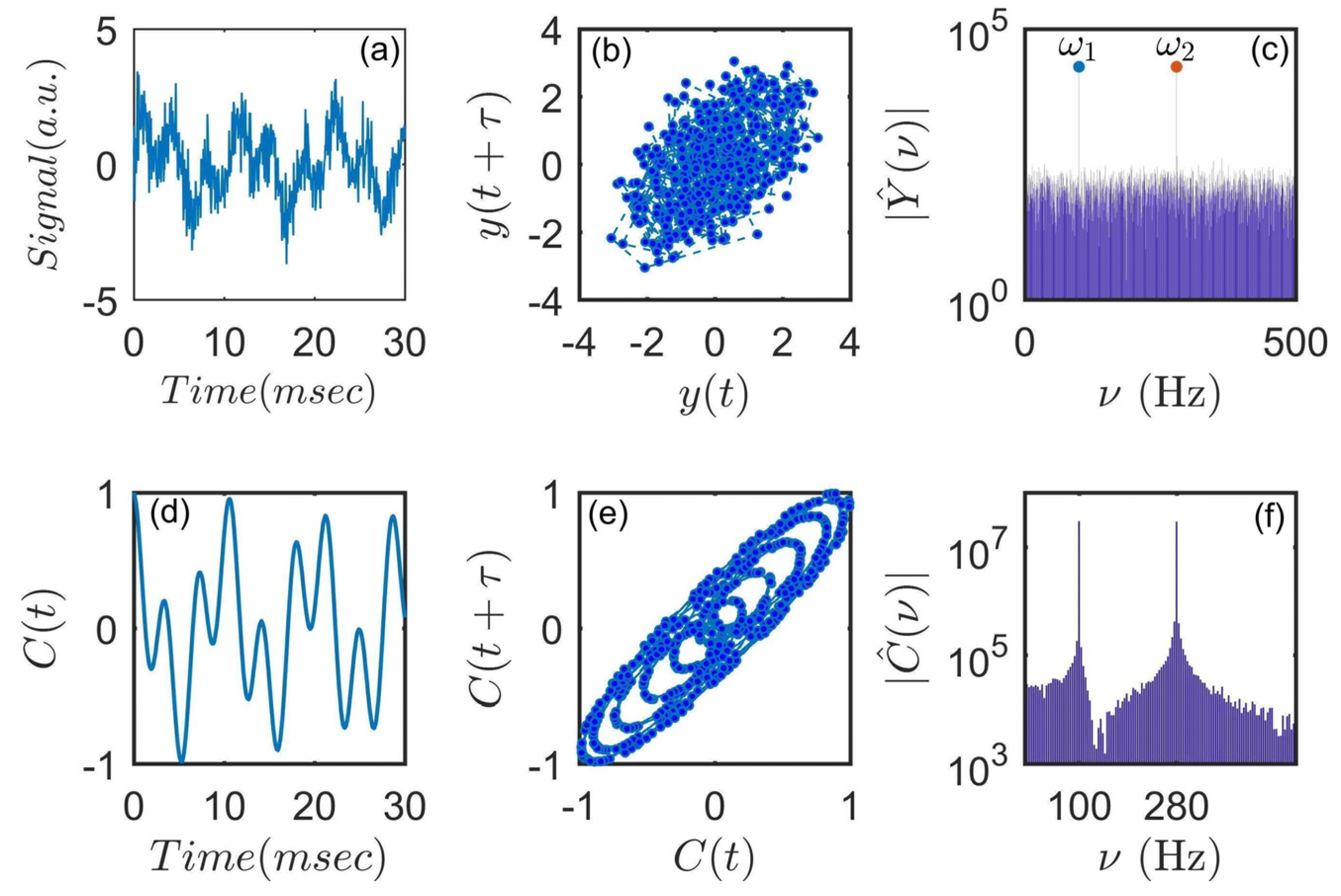
3.1. Introduction to Correlation Analysis

One approach to circumvent the extremely slow irregular drift in the signal is through the use of auto-correlation or cross-correlation functions (for multi-point signals). The latter is defined as [44,45]:
C r , r ' ; τ = f ( r ; t ) f ( r ; t + τ ) t ο f r · ο f r
where ο [ f ( r ) ] represents the standard deviation of the signal f ( r ; t ) , which is mean centered. The auto-correlation function for the signal from a single transducer at r is C r , r ; τ .
We propose the use of correlation functions to establish the low-dimensionality (or lack thereof) of the dynamics. Two observations motivate their use: First, the statistical means of t - average out high-frequency noise in the time series. Second, slow variations in the time-series baseline are irrelevant for sufficiently small τ . By reducing both high and low frequency noise, we are in a better position to test for the low/high dimensionality of the signal. However, it is important to note that we are unable to deduce the dynamics of the time-series variable through correlation functions.
Prior to implementing correlation analysis on experimental data, we study its application to a synthetic time series with similar spectral characteristics as the experimental pressure signal. We consider a signal comprised of frequencies of 100 & 280 Hz, to which we add Gaussian noise. Time series shown in Figure 6a corresponds to Gaussian noise (SNR = 2); the signal is sampled at 20 kHz to simulate the sampling frequency of the pressure transducers. The Fourier spectrum and space-filling phase-space orbit appear to be qualitatively similar to the experimental signal (Figure 6b,c). However, both the power spectra and phase space appear to be rectified once the signal is subjected to correlation analysis. Auto-correlation of the synthetic data and the corresponding phase space and power spectrum are shown in Figure 6d–f. Even when the signal-to-noise ratio is small, time series of the auto-correlation is able to successfully reveal the underlying quasi-periodic dynamics of the signal.

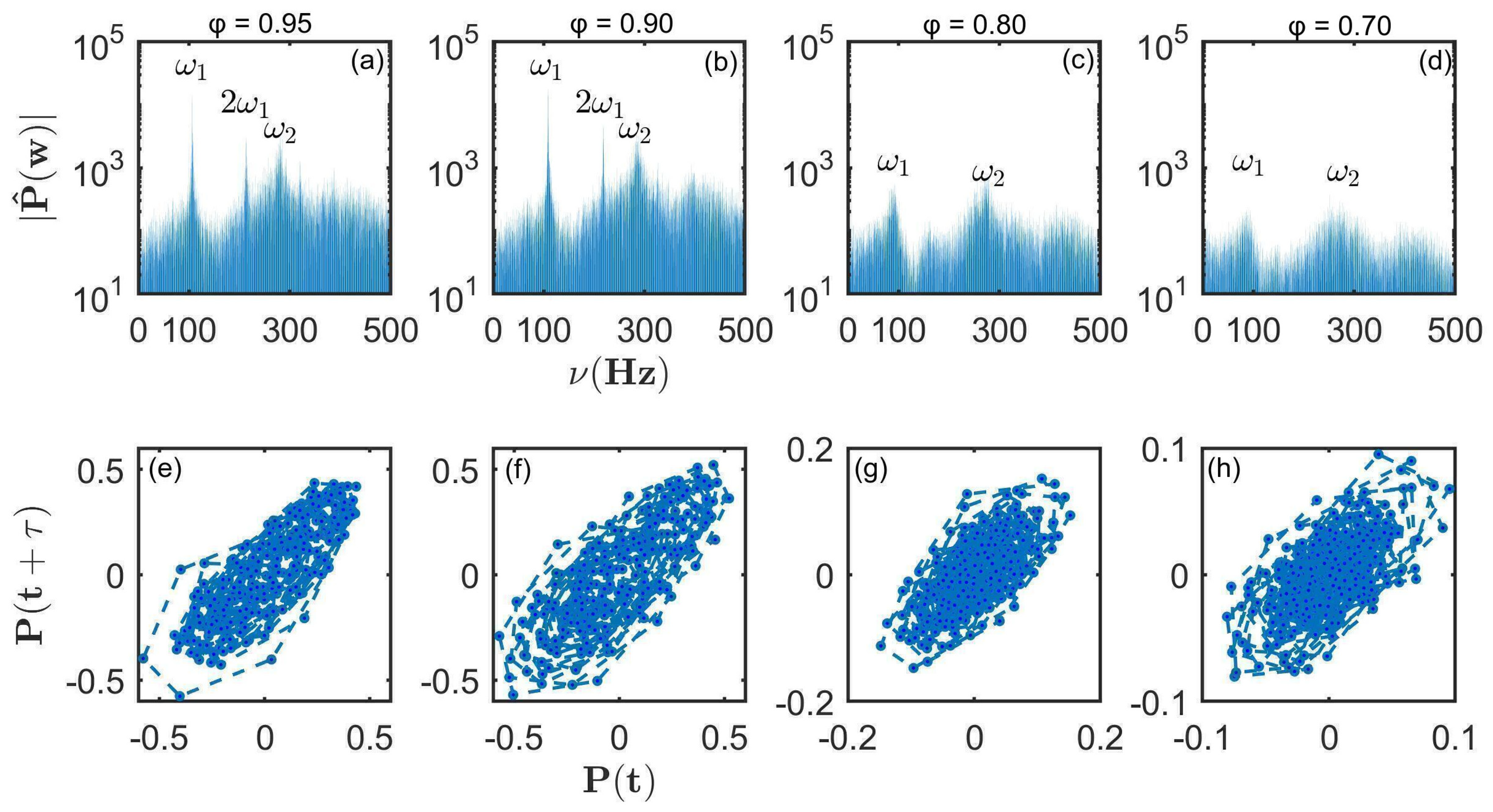
3.2. Autocorrelation Function of Bluff Body Pressure Time Series

Conducive findings from the analysis of the synthetic data motivate the use of correlation analysis to experimental time series. Auto-correlation functions as a function of the time-delay τ and their power spectra for flows at T = 440 F are shown in Figure 7, with the same equivalence ratios as in Figure 3. Prior to the onset of the secondary instability, the auto-correlation function C r , r ; τ ,  Figure 7a,b, appears to be periodic in τ , and the time-delay dynamics, Figure 7e,f, low dimensional. The level of broadband noise, Figure 7i,j, has reduced. These observations can be interpreted as follows. Prior to onset of asymmetric shedding, the major flow constituent is periodic, although the time series has significant levels of high and low frequency noise.
The auto-correlation function (Figure 7c,d) and power spectrum (Figure 7k,l) indicate that the flow following the onset of the secondary instability represent noisy quasi-periodic flow; further, the spectra show that the two associated frequencies are ω 1 and ω 2 . However, noise-reduction achieved through the use of auto-correlation function is insufficient to highlight the quasi-periodic nature of the time-delay plot. We also note the presence of a ω 2 -component of the signal even prior to the onset of the secondary instability. Presumably the downstream growth of the asymmetric vortex shedding requires the amplitude of the mode to be finite, suggesting that the transition is sub-critical. Similar behavior is observed in flows at other temperatures.

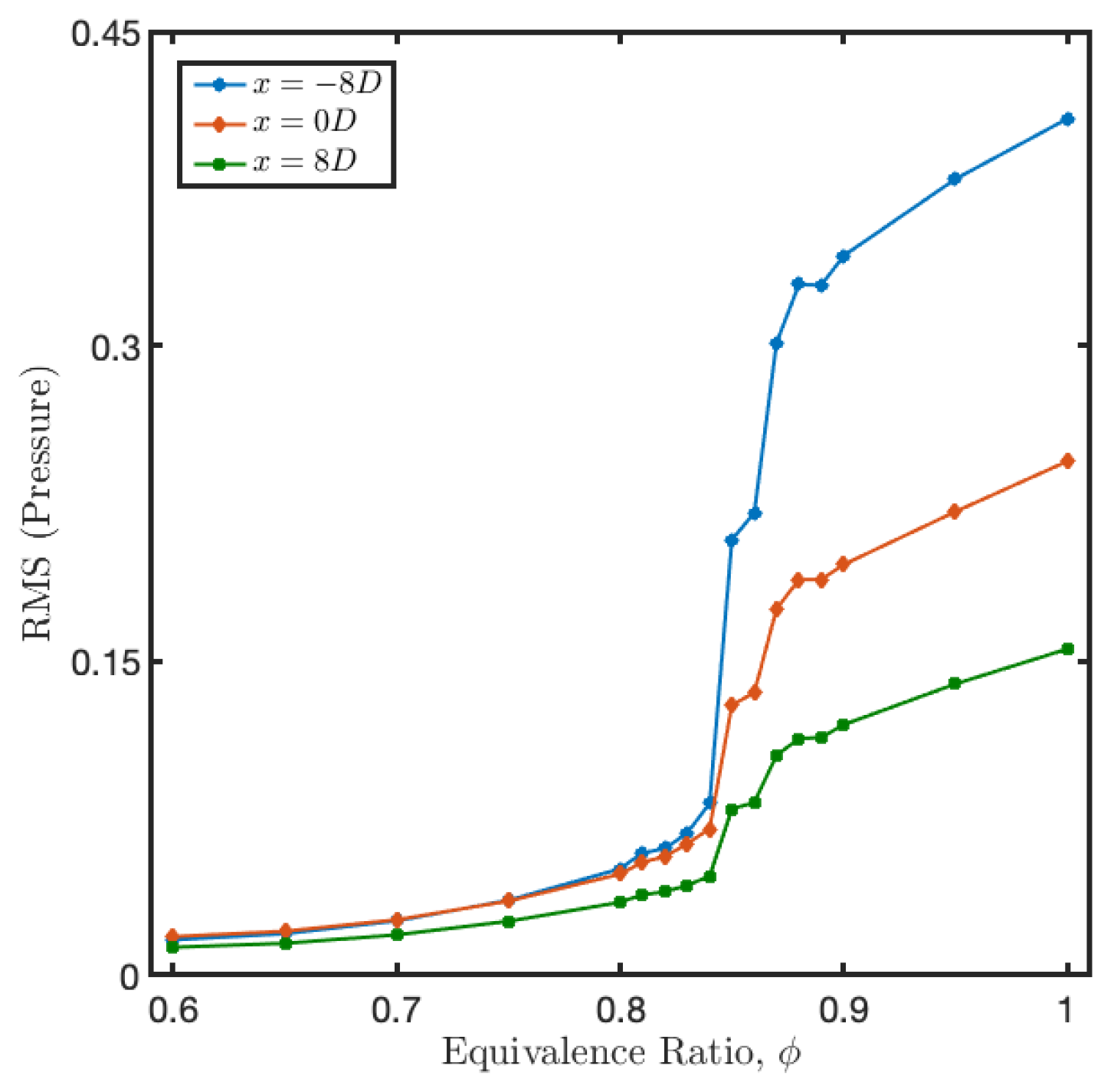
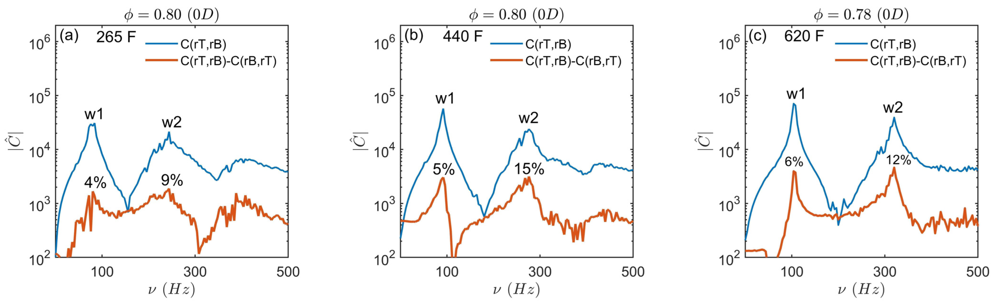
3.3. Growth of the Asymmetric Mode with Equivalence Ratio at Various Inlet Temperature Conditions

To conclude this section, we illustrate an additional utility of auto-correlation functions; specifically, to characterize the growth of the secondary instability. The relevant measure is the ratio of spectral contributions from the asymmetric secondary instability (frequency ω 2 ) and the symmetric primary instability (frequency ω 1 ) as the equivalence ratio is reduced φ = 1.00 to φ = 0.60 . Spectral contributions or ‘strengths’ of   ω 1 and   ω 2 are obtained from the power spectrum of auto-correlation. As shown in Figure 8, the ratio nearly vanishes prior to the onset of the asymmetric shedding, and grows beyond onset. Further, asymmetric shedding dominates the flow at low equivalence ratios.
We extend our analysis to explore the growth of the asymmetric secondary instability (frequency ω 2 ) for a range temperature condition from 100 F up to 620 F. For all the temperatures, the trend is similar. Ratio of the peaks obtained from the auto-correlation function gradually grows up as the equivalence ratio is scaled down from 1.0 to 0.6.

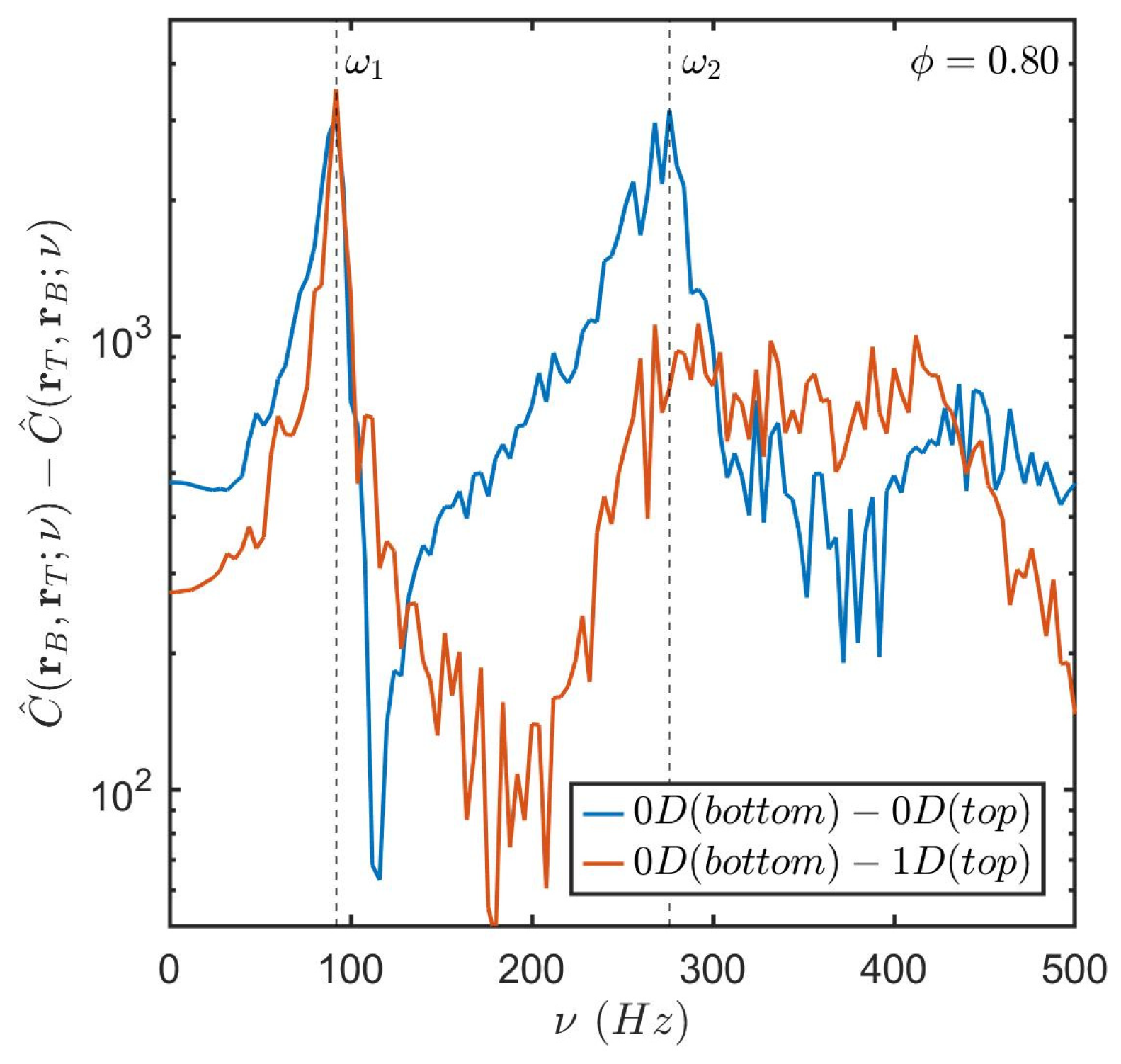
4. Cross-Correlation Functions of Bluff-Body Pressure Time Series

Clearly, spatial features of flow constituents cannot be extracted from a single time series; however, as we show in this section, cross-correlation function between signals from appropriately placed transducers can be used to establish symmetries in flow constituents. Pressure variations due to symmetric vortex shedding on any transducer are periodic; harmonics of the fundamental frequency can be expected to increase downstream as highly nonlinear vortices develop. In the absence of noise, time series from the symmetric vortex shedding at transducers located on the top and bottom surfaces at the same axial location will be identical. In asymmetric vortex shedding, vortices are once again shed periodically, however from alternate sides of the bluff body. There is no symmetry between time series at the top and bottom transducers. We show in Appendix A how these differences in signals from transducers placed at the top and bottom surfaces can be used to differentiate between the signals from the two classes of shedding.
The quantity of interest is Δ C C r T ,   r B ; τ C r B ,   r T ; τ , where C r T ,   r B ; τ represents the cross-correlation between the signal of time series from a transducer at the site r T on the top surface, and the time-delayed signal from a transducer at r B , the symmetrically-located point on the bottom surface. Ideally, frequency content associated with symmetric flow constituents should be suppressed completely in the cross-correlation difference ( Δ C ). However, likely due to noise and nonlinear coupling of vortices, the cancellation was imperfect. Nonetheless, one can expect a larger drop of symmetric components in Δ C than the asymmetric components. We investigate the percentages of ω 1 and ω 2 strengths in Δ C relative to those in C r T ,   r B ; τ . As shown in Figure 9, it is observed that, regardless of the inlet temperature condition, percentage of ω 2 in Δ C is higher than that of ω 1 compared to C r T ,   r B ; τ . For example, in case of 265 F, ω 2 for Δ C is 9% of C r T ,   r B ; τ , whereas ω 1 for Δ C is only 4% of C r T ,   r B ; τ ). This behavior is persistent at lower equivalence ratios as well (Figure 10). Therefore, difference of cross-correlation enables distinguishing the time-delayed anti-symmetric flow-constituents from asymmetric ones, something that was not obvious from only cross-correlation. Thus, the presence or absence of spatial symmetries in the flow constituents can be established using time series from two transducers.
The use of Δ C required the presence/absence of up/down symmetry in the two constituents. This difference can only be extracted using appropriate placement of transducers. To elaborate, we show in Figure 11 the behavior of Δ C ^ = | C ^ r T ,   r B ; τ C ^ r B ,   r T ; τ | for time-series from the transducer at 0D on the bottom surface and 1D at the top surface. Here, the ω 2 component fails to be enhanced. To reiterate, cross-correlation analyses of time series from appropriately placed transducers can be used to establish spatial symmetries of flow constituents.
It should be noted that secondary instability ( ω 2 ) might be a separate combustion mode itself, sometimes which is close to 3 ω 1 but generally not. When bluff body responds to the acoustic field through vortex shedding, ω 2 usually couples back to ω 1 , that we believe to be a reason as to why ω 1 doesn’t cancel out in the difference of cross-correlation, Δ C ^ . If it’s exactly symmetric, it should cancel.
To strengthen our findings, we refer to the previous work of Roy et al. [46], where they investigated the similar instabilities of bluff body vortices applying robust Dynamic Mode Decomposition (DMD) analysis on two-dimensional images of hydroxyl (OH) behind a bluff body acquired utilizing the PLIF technique. They were able to differentiate between these symmetric and asymmetric shedding analyzing the OH-PLIF images at various equivalence ratios. Unfortunately, these advanced measurement imaging tools are not routinely available in most laboratories; the standard measurement devices used to study fluid flows in nearly every laboratory are transducers, which provide high-frequency single point or multi-point measurements of flow variables. The questions we address in this work is what inferences on the underlying flows can be made on the basis of multi-point measurements utilizing correlation analysis.

5. Discussion

Preventing the onset and growth of instabilities in fluid and combustion flows is critical to optimize their performance. The absence of simple boundary conditions and symmetries in realistic configurations often precludes analytical studies of these systems. The existence of structures on a vast range of scales in strongly driven flows makes computational studies intractable as well. The most promising approach to establish flow constituents and instabilities is via experimental data. Unfortunately, experimental data contains noise, and the task of extracting the primary flow constituents becomes a nontrivial task. Noise levels are especially high in combustion flows, which are enhanced by sensitive dependence on initial conditions.
In this work, we introduce a pair of approaches to reduce noise and to establish geometric and dynamic features of the primary flow constituents. They were illustrated in combustion flows within a configuration of rectangular cross section and passing a symmetric bluff body. Flow instabilities in such symmetric configurations are known and thus conclusions made on the basis of our studies can be independently validated. However, we emphasize that techniques outlined here do not rely on these symmetries. The data used for the analysis were pressure time-series from 9 transducers, 6 of which were placed on the bottom surface, and 3 on the top surface. One transducer on the top surface was at the axial location of the trailing edge of the bluff body and two downstream of it. Three of the 6 transducers on the bottom surface were at identical axial locations. Hence it was possible to test for symmetries in the flow constituents. The time-series from each transducer was taken at 20 kHz over a 20 s interval.
There is a significant level of high and low frequency noise in the data, as can be inferred from power spectra and time-delay plots. Standard filtering algorithms failed to improve the spectra or time-delayed plots to identify possible low-dimensionality of the dynamics. Our proposal is to use auto-correlation and cross-correlation functions as a function of time delay to determine the low dimensionality (or lack thereof) of the dynamics associated with primary flow constituents. The use of correlation function, through time averages, reduces high-frequency noise. Evaluating them for sufficiently small time delays τ prevents effects of slow variations in the baseline caused by feedback. (For example, heat emission in combustion can increase the temperature of the configuration, thus affecting experimental conditions.) These expectations are validated in combustion flows behind the bluff body. Prior to the onset of asymmetric vortex shedding, the auto-correlation function C r , r ; τ is periodic in τ, and the time-delay plots of the auto-correlation function (i.e., C r , r ; τ   vs   C ( r , r ; τ + τ 0 ) ) appear (nearly) periodic. Its power spectrum is most intense at a frequency, ω 1 100   H z . Auto-correlation function following the onset exhibits characteristics of noisy quasi-periodic behavior, and its power spectrum contains a second peak around ω 2 280   H z . We show how cross correlation functions of time series from symmetrically placed transducers can be used to establish symmetries of the flow constituents. The relevant measure is Δ C C r T ,   r B ; τ C r B ,   r T ; τ , the difference between cross correlation functions between the two time series, which suppresses the frequency content associated with symmetric flow constituents. Although the cancellation of symmetric components was imperfect, likely due to noise and vortex coupling, a larger drop of ω 1 component is observed in Δ C than the asymmetric ω 2 component. We thus inferred that flow constituents with frequencies ω 1 and ω 2 were symmetric and asymmetric vortex shedding respectively. Furthermore, a smaller component of frequency ω 2 is found even prior to the onset of asymmetric shedding, suggesting that the transition is sub-critical.

6. Conclusive Summary

Identifying dominant flow components is essential for understanding the underlying dynamics and effectively controlling complex flows. We demonstrate how correlation functions (either auto-correlation functions for single time-series or cross-correlation functions for multiple time-series) can be strategically employed to reveal the dynamic behavior of the primary flow components by effectively reducing the stubborn noisy features. Methodologies presented here are not dependent on special features, such as uniform boundaries or symmetries, of the experimental configuration. Consequently, the analysis is expected to be applicable to more general configurations. One potentially important example is the detection of changes to flow characteristics in (for example) airplane engines using data from embedded transducers. Such changes could signal imminent damage to the engine from non-visualizable changes such as fatigue or wear-and-tear.

Author Contributions

A.S.: Conceptualization, Data curation, Formal analysis, Investigation, Methodology, Visualization, Writing—original draft, Writing—review & editing. H.S.: Conceptualization, Methodology, Visualization, Writing—original draft, Writing—review & editing. All authors have read and agreed to the published version of the manuscript.

Funding

This research received no specific grant from any funding agency.

Data Availability Statement

The data presented in this study are available on request from the corresponding author.

Acknowledgments

The authors gratefully acknowledge the technical support of Douglas G. Talley, Andrew Caswell, Gemunu Gunaratne, Sukesh Roy, Chris Fugger and Terrence Meyer. The authors are grateful to the School of Mechanical Engineering, Purdue University for providing the computational resources.

Conflicts of Interest

The authors declare that they have no known competing financial interests or personal relationships that could have appeared to influence the work reported in this paper.

Appendix A. Differentiating Symmetric and Time-Delayed Anti-Symmetric Constituents

Consider transducer measurements of the bluff-body flow, made from two points on the upper and lower surfaces, at the same axial location. Suppose the signals at the transducers were due to a symmetric (i.e., identical at the upper and lower surfaces) component g S ( t ; ω 1 ) and to a time-delayed asymmetric (i.e., von Karman shedding) component g A ( t ; ω 2 ), where the notation signifies that the two signals have frequencies ω 1 and ω 2 respectively. (As we see below these are the frequencies identified from the spectral analysis of the signal and the auto-correlation function.) The time-shifted signal at the bottom transducer due to the second signal is g A ( t + π / ω 2 ; ω 2 ). Under these assumptions, overall signals on the top and bottom transducers, whose locations are denoted r T and r B are
f r T ; t = g S t ; ω 1 + g A t ; ω 2 + η T t
f r B ; t = g S t ; ω 1 + g A t + π ω 2 ; ω 2 + η B t
where η T t and η B t represent the noise on the top and bottom transducers. The cross-correlation function is
C r T ,   r B ; τ = f r T ; t · f r B ; t + τ ο f r T · ο f r B
In order to simplify the expression, we note first that when the frequencies ω 1 and ω 2 are incommensurate, g S t ; ω 1 · g A t + π / ω 2 ; ω 2 vanishes. This is most easily seen by Fourier expanding the fields,
g S t ; ω 1 = m g ^ S m e 2 π i m ω 1 t
g A t ; ω 2 = n g ^ A n e 2 π i n ω 2 t
and noting that
g S t ; ω 1 · g A t + τ ; ω 2 = m , n g ^ S m g ^ A n e 2 π i n ω 2 τ e 2 π i m ω 1 + n ω 2 t
Since ω 1 and ω 2 are incommensurate, m , n m ω 1 + n ω 2 0 , and hence, e 2 π i ( m ω 1 + n ω 2 ) t = 0 ; thus, g S t ; ω 1 · g A t ; ω 2 = 0 .
Second, we assume that noise is uncorrelated to the signals g S t ; ω 1 and g A t ; ω 2 , i.e., g S , A t ; ω 1 · η T , B t = 0 . If this were the case (an unlikely case, as we point out later),
C r T ,   r B ; τ = g S t ; ω 1 · g S t + τ ; ω 1 + g A t ; ω 2 · g A t + π ω 2 + τ ; ω 2 ο f r T · ο f r B
Subtracting from the corresponding expression for C r B ,   r T ; τ expresses the difference Δ C as
Δ C = g A t ; ω 2 · g A t + π ω 2 + τ ; ω 2 g A t + τ ; ω 2 · g A t + π ω 2 ; ω 2 ο f r T · ο f r B   ,
implying that the signal Δ C has no spectral components at ω 1 . Realistically, noise in fluid systems is rarely uncorrelated to the flow dynamics; for example, velocity gradients, and hence energy cascades to smaller scales, is large near vortices and eddies. Consequently, the levels of pressure fluctuation at such sites may be expected to be larger as well. However, if the frequency ω 2 results from an asymmetric signal, one may expect the corresponding spectral component of Δ C to be relatively large compared to that in C r T ,   r B ; τ .

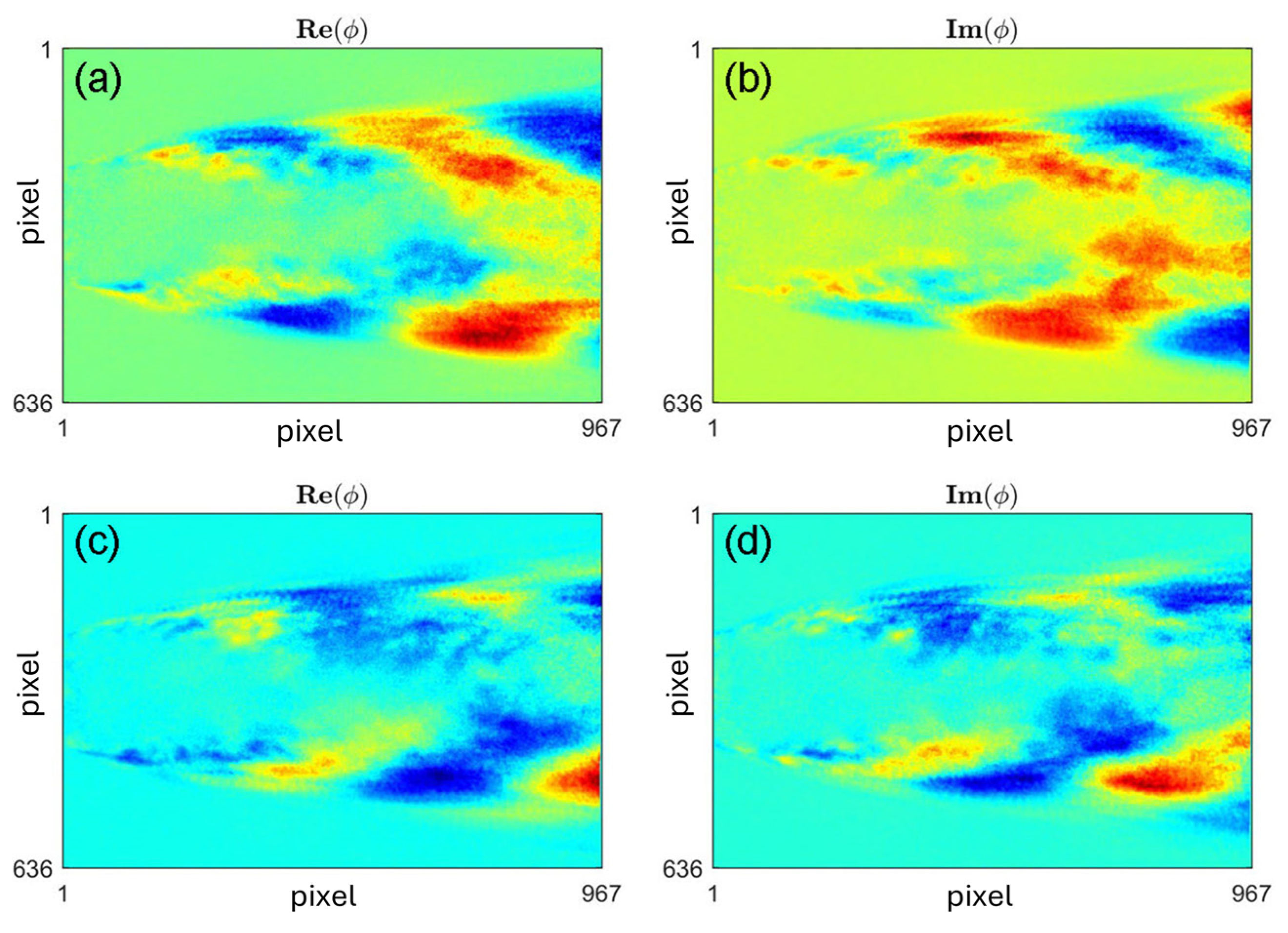
Appendix B. Dynamic Mode Decomposition Applied to Spatio-Temporal Data

Dynamic mode decomposition (DMD) is a standard technique of identifying ‘coherent structures’ by analyzing fluid or combustion flows [47,48,49], unlike Proper Orthogonal Decomposition (POD), which categorizes coherent structures according to correlations. Each DMD mode corresponds to a spatial structure that oscillates with a single frequency, making it a natural approach to extract periodic flow constituents, such as symmetric or asymmetric vortex shedding. Robust DMD, an effective extension of conventional DMD, aims to identify robust (configuration-independent) and non-robust constituents of the flow. Characterizing robust constituents is crucial to develop reduced-order models as well as to control the flow. Detailed mathematical explanations and applications of robust DMD analysis can be found in [46,50,51].
Roy et al. [46] reported the symmetric and asymmetric modes obtained by utilizing robust DMD analysis on the OH-PLIF images of bluff body vortex shedding. At a low equivalence ratio of φ = 0.8, they were able to identify both symmetric and asymmetric flow constituents. In the current study, we have been able to detect similar symmetric and asymmetric instabilities utilizing correlation analysis of the pressure transducer data. We also repeated robust DMD calculation using available OH-PLIF imaging data and detected similar instability modes (Figure A1) obtained by Roy et al. [46].
Figure A1. Robust DMD analysis on bluff body OH-PLIF imaging data. (a) Real and (b) imaginary parts of the symmetric mode Φ (x) with the largest energy, for the reacting flow at equivalence ratio 0.8. Pair of vortices shed periodically from both edges of the bluff body. (c) Real and (d) imaginary parts of the asymmetric mode with the highest energy, where the vortices shed periodically from alternate edges of the bluff body. (Flow direction is from left to right).
Mca 30 00068 g0a1

References

  1. Lieuwen, T.C. Unsteady Combustor Physics; Cambridge University Press: Cambridge, UK, 2021. [Google Scholar]
  2. Seshadri, A.; Pavithran, I.; Unni, V.R.; Sujith, R.I. Predicting the Amplitude of Limit-Cycle Oscillations in Thermoacoustic Systems with Vortex Shedding. AIAA J. 2018, 56, 3507–3514. [Google Scholar] [CrossRef]
  3. Pavithran, I.; Unni, V.R.; Varghese, A.J.; Sujith, R.; Saha, A.; Marwan, N.; Kurths, J. Universality in the emergence of oscillatory instabilities in turbulent flows. EPL (Europhys. Lett.) 2020, 129, 24004. [Google Scholar] [CrossRef]
  4. Dupe`re, I.D.J.; Dowling, A.P. The Use of Helmholtz Resonators in a Practical Combustor. J. Eng. Gas Turbines Power 2005, 127, 268–275. [Google Scholar] [CrossRef]
  5. Dawson, J.R.; Worth, N.A. The effect of baffles on self-excited azimuthal modes in an annular combustor. Proc. Combust. Inst. 2015, 35, 3283–3290. [Google Scholar] [CrossRef]
  6. Waesche, R.H.W. Mechanisms and Methods of Suppression of Combustion Instability by Metallic Additives. J. Propuls. Power 1999, 15, 919–922. [Google Scholar] [CrossRef]
  7. Lieuwen, T.; Shanbhogue, S.; Khosla, S.; Smith, C. Dynamics of bluff body flames near blowoff. In Proceedings of the 45th AIAA Aerospace Sciences Meeting and Exhibit, Reno, NV, USA, 8–11 January 2007. [Google Scholar]
  8. Shanbhogue, S.J.; Husain, S.; Lieuwen, T. Lean blowoff of bluff body stabilized flames: Scaling and dynamics. Prog. Energy Combust. Sci. 2009, 35, 98–120. [Google Scholar] [CrossRef]
  9. Kostka, S.; Lynch, A.C.; Huelskamp, B.C.; Kiel, B.V.; Gord, J.R.; Roy, S. Characterization of flame-shedding behavior behind a bluff-body using proper orthogonal decomposition. Combust. Flame 2012, 159, 2872–2882. [Google Scholar] [CrossRef]
  10. Shanbhogue, S.; Plaks, D.; Lieuwen, T. The KH instability of reacting, acoustically excited bluff body shear layers. In Proceedings of the 43rd AIAA/ASME/SAE/ASEE Joint Propulsion Conference & Exhibit, Cincinnati, OH, USA, 8–11 July 2007. [Google Scholar]
  11. Kandlikar, S.G.; Joshi, S.; Tian, S. Effect of Surface Roughness on Heat Transfer and Fluid Flow Characteristics at Low Reynolds Numbers in Small Diameter Tubes. Heat Transf. Eng. 2003, 24, 4–16. [Google Scholar] [CrossRef]
  12. Kim, D.E.; Kim, M.H. Experimental study of the effects of flow acceleration and buoyancy on heat transfer in a supercritical fluid flow in a circular tube. Nucl. Eng. Des. 2010, 240, 3336–3349. [Google Scholar] [CrossRef]
  13. Kabiraj, L.; Sujith, R. Nonlinear self-excited thermoacoustic oscillations: Intermittency and flame blowout. J. Fluid Mech. 2012, 713, 376–397. [Google Scholar] [CrossRef]
  14. Chiam, Z.L.; Lee, P.S.; Singh, P.K.; Mou, N. Investigation of fluid flow and heat transfer in wavy micro-channels with alternating secondary branches. Int. J. Heat Mass Transf. 2016, 101, 1316–1330. [Google Scholar] [CrossRef]
  15. Kunze, K.; Hirsch, C.; Sattelmayer, T. Transfer Function Measurements on a Swirl Stabilized Premix Burner in an Annular Combustion Chamber; American Society of Mechanical Engineers Digital Collection: New York, NY, USA, 2008; pp. 21–29. [Google Scholar] [CrossRef]
  16. Kim, D.; Lee, J.G.; Quay, B.D.; Santavicca, D.A.; Kim, K.; Srinivasan, S. Effect of Flame Structure on the Flame Transfer Function in a Premixed Gas Turbine Combustor. J. Eng. Gas Turbines Power 2009, 132, 021502. [Google Scholar] [CrossRef]
  17. Zhang, M.; Wang, J.; Xie, Y.; Wei, Z.; Jin, W.; Huang, Z.; Kobayashi, H. Measurement on instantaneous flame front structure of turbulent premixed CH4/H2/air flames. Exp. Therm. Fluid Sci. 2014, 52, 288–296. [Google Scholar] [CrossRef]
  18. Fojtlín, M.; Planka, M.; Fišer, J.; Pokorný, J.; Jícha, M. Airflow Measurement of the Car HVAC Unit Using Hot-Wire Anemometry. EPJ Web Conf. 2016, 114, 02023. [Google Scholar] [CrossRef]
  19. Kalpakli Vester, A.; Sattarzadeh, S.S.; Örlü, R. Combined hot-wire and PIV measurements of a swirling turbulent flow at the exit of a 90° pipe bend. J. Vis. 2016, 19, 261–273. [Google Scholar] [CrossRef]
  20. Kwon, S.Y.; Lee, S. Precise measurement of thermal conductivity of liquid over a wide temperature range using a transient hot-wire technique by uncertainty analysis. Thermochim. Acta 2012, 542, 18–23. [Google Scholar] [CrossRef]
  21. Minakov, A.V.; Rudyak, V.Y.; Guzei, D.V.; Pryazhnikov, M.I.; Lobasov, A.S. Measurement of the Thermal-Conductivity Coefficient of Nanofluids by the Hot-Wire Method. J. Eng. Phys. Thermophys. 2015, 88, 149–162. [Google Scholar] [CrossRef]
  22. Azarfar, S.; Movahedirad, S.; Sarbanha, A.A.; Norouzbeigi, R.; Beigzadeh, B. Low cost and new design of transient hot-wire technique for the thermal conductivity measurement of fluids. Appl. Therm. Eng. 2016, 105, 142–150. [Google Scholar] [CrossRef]
  23. Li, F.; Shi, S.; Ma, W.; Zhang, X. A switched vibrating-hot-wire method for measuring the viscosity and thermal conductivity of liquids. Rev. Sci. Instrum. 2019, 90, 075105. [Google Scholar] [CrossRef]
  24. Mylona, S.K.; Yang, X.; Hughes, T.J.; White, A.C.; McElroy, L.; Kim, D.; Al Ghafri, S.; Stanwix, P.L.; Sohn, Y.H.; Seo, Y.; et al. High-Pressure Thermal Conductivity Measurements of a (Methane + Propane) Mixture with a Transient Hot-Wire Apparatus. J. Chem. Eng. Data 2020, 65, 906–915. [Google Scholar] [CrossRef]
  25. Saha, A.; Crosmer, J.; Roy, S.; Meyer, T.R. Spatio-temporal dynamics of an acoustically forced cryogenic coaxial jet injector. Int. J. Multiph. Flow 2024, 170, 104627. [Google Scholar] [CrossRef]
  26. Bendat, J.S.; Piersol, A.G. Random Data: Analysis and Measurement Procedures; John Wiley & Sons: Hoboken, NJ, USA, 2011. [Google Scholar]
  27. da Cunha Lima, A.T.; da Cunha Lima, I.C.; de Almeida, M.P. Analysis of turbulence power spectra and velocity correlations in a pipeline with obstructions. Int. J. Mod. Phys. C 2016, 28, 1750019. [Google Scholar] [CrossRef]
  28. Takens, F. Detecting strange attractors in turbulence. In Dynamical Systems and Turbulence, Warwick 1980; Springer: Berlin/Heidelberg, Germany, 1981; pp. 366–381. [Google Scholar]
  29. Cross, M.C.; Hohenberg, P.C. Pattern formation outside of equilibrium. Rev. Mod. Phys. 1993, 65, 851. [Google Scholar] [CrossRef]
  30. Kabiraj, L.; Saurabh, A.; Wahi, P.; Sujith, R. Route to chaos for combustion instability in ducted laminar premixed flames. Chaos Interdiscip. J. Nonlinear Sci. 2012, 22, 023129. [Google Scholar] [CrossRef] [PubMed]
  31. Basarab, M.A.; Konnova, N.S.; Basarab, D.A.; Matsievskiy, D.D. Digital signal processing of the Doppler blood flow meter using the methods of nonlinear dynamics. In Proceedings of the 2017 Progress in Electromagnetics Research Symposium—Spring (PIERS), St. Petersburg, Russia, 22–25 May 2017. [Google Scholar] [CrossRef]
  32. Fric, T.F.; Roshko, A. Vortical structure in the wake of a transverse jet. J. Fluid Mech. 1994, 279, 1–47. [Google Scholar] [CrossRef]
  33. Lee, I.; Sung, H.J. Multiple-arrayed pressure measurement for investigation of the unsteady flow structure of a reattaching shear layer. J. Fluid Mech. 2002, 463, 377–402. [Google Scholar] [CrossRef]
  34. Hudy, L.M.; Naguib, A.; Humphreys, W.M. Stochastic estimation of a separated-flow field using wall-pressure-array measurements. Phys. Fluids 2007, 19, 024103. [Google Scholar] [CrossRef]
  35. Sherry, M.; Jacono, D.; Sheridan, J.; Mathis, R.; Marusic, I. Flow separation characterisation of a forward facing step immersed in a turbulent boundary layer. In Proceedings of the 6th International Symposium on Turbulence and Shear Flow Phenomena, Seoul, Republic of Korea, 22–24 June 2009. [Google Scholar] [CrossRef]
  36. Awasthi, M.; Devenport, W.J.; Glegg, S.A.L.; Forest, J.B. Pressure fluctuations produced by forward steps immersed in a turbulent boundary layer. J. Fluid Mech. 2014, 756, 384–421. [Google Scholar] [CrossRef]
  37. Wu, S.J.; Miau, J.J.; Hu, C.C.; Chou, J.H. On low-frequency modulations and three-dimensionality in vortex shedding behind a normal plate. J. Fluid Mech. 2005, 526, 117–146. [Google Scholar] [CrossRef]
  38. Xu, S.J.; Zhou, Y.; Wang, M.H. A symmetric binary-vortex street behind a longitudinally oscillating cylinder. J. Fluid Mech. 2006, 556, 27–43. [Google Scholar] [CrossRef]
  39. Behera, N.; Agarwal, V.K.; Jones, M.; Williams, K.C. Power Spectral Density Analysis of Pressure Fluctuation in Pneumatic Conveying of Powders. Part. Sci. Technol. 2015, 33, 510–516. [Google Scholar] [CrossRef]
  40. Fugger, C.A.; Roy, S.; Caswell, A.W.; Rankin, B.A.; Gord, J.R. Structure and dynamics of CH2O, OH, and the velocity field of a confined bluff-body premixed flame, using simultaneous PLIF and PIV at 10 kHz. Proc. Combust. Inst. 2019, 37, 1461–1469. [Google Scholar] [CrossRef]
  41. Heitor, M.; Taylor, A.; Whitelaw, J. Influence of confinement on combustion instabilities of premixed flames stabilized on axisymmetric baffles. Combust. Flame 1984, 57, 109–121. [Google Scholar] [CrossRef]
  42. Faltinsen, O.M.; Timokha, A.N. Sloshing; Cambridge University Press: Cambridge, UK, 2009. [Google Scholar]
  43. Saha, A.; Subramani, H.; Meyer, T.R.; Gunaratne, G.; Yi, T.; Roy, S. Analysis of Spatiotemporal Data. In Optical Diagnostics for Reacting and Non-Reacting Flows: Theory and Practice; American Institute of Aeronautics and Astronautics, Inc.: Reston, VA, USA, 2022; pp. 1203–1288. [Google Scholar] [CrossRef]
  44. Bourgoin, M.; Baudet, C.; Kharche, S.; Mordant, N.; Vandenberghe, T.; Sumbekova, S.; Stelzenmuller, N.; Aliseda, A.; Gibert, M.; Roche, P.-E.; et al. Investigation of the small-scale statistics of turbulence in the Modane S1MA wind tunnel. CEAS Aeronaut. J. 2018, 9, 269–281. [Google Scholar] [CrossRef]
  45. Yanovych, V.; Duda, D.; Uruba, V.; Antoš, P. Anisotropy of turbulent flow behind an asymmetric airfoil. SN Appl. Sci. 2021, 3, 885. [Google Scholar] [CrossRef]
  46. Roy, S.; Hua, J.-C.; Barnhill, W.; Gunaratne, G.H.; Gord, J.R. Deconvolution of reacting-flow dynamics using proper orthogonal and dynamic mode decompositions. Phys. Rev. E 2015, 91, 013001. [Google Scholar] [CrossRef]
  47. Rowley, C.W.; Mezić, I.; Bagheri, S.; Schlatter, P.; Henningson, D.S. Spectral analysis of nonlinear flows. J. Fluid Mech. 2009, 641, 115–127. [Google Scholar] [CrossRef]
  48. Schmid, P.J. Dynamic mode decomposition of numerical and experimental data. J. Fluid Mech. 2010, 656, 5–28. [Google Scholar] [CrossRef]
  49. Tu, J.H.; Rowley, C.W.; Luchtenburg, D.M.; Brunton, S.L.; Kutz, J.N. On dynamic mode decomposition: Theory and applications. J. Comput. Dyn. 2014, 1, 391. [Google Scholar] [CrossRef]
  50. Roy, S.; Yi, T.; Jiang, N.; Gunaratne, G.; Chterev, I.; Emerson, B.; Lieuwen, T.; Caswell, A.; Gord, J. Dynamics of robust structures in turbulent swirling reacting flows. J. Fluid Mech. 2017, 816, 554–585. [Google Scholar] [CrossRef]
  51. Hua, J.-C.; Gunaratne, G.H.; Talley, D.G.; Gord, J.R.; Roy, S. Dynamic-mode decomposition based analysis of shear coaxial jets with and without transverse acoustic driving. J. Fluid Mech. 2016, 790, 5–32. [Google Scholar] [CrossRef]
Figure 1. Schematic of the bluff body combustion chamber with locations of pressure transducers. The trailing edge of the symmetric bluff body is assigned to be at x = 0 , downstream locations being positive. Note that transducers 7, 8, and 9 are placed opposite to 4, 5, and 6 respectively.
Mca 30 00068 g001
Figure 2. Root-mean-square pressure fluctuations. The central curve shows the RMS pressure variation for the transducer at x = 0 as a function of the equivalence ratio φ for combustion flows at T = 440 F. Blue (upper) and green (lower) curves correspond to RMS values for transducers at x = 8 D and x = + 8 D .
Mca 30 00068 g002
Figure 3. Flow characteristics of the signal. Power spectra (ad) and time-delayed plots (eh) for representative combustion flows at 440 F. Plots (a,b,e,f) correspond to equivalence ratios φ = 0.95 and 0.90, prior to the onset of asymmetric vortex shedding, while (c,d,g,h) correspond to φ =0.80 and 0.70 respectively, following the onset. At the larger φ : (a,b) the flow is found to have sharp spectral peaks at frequencies ω 1 110   H z , 2 ω 1 , and ω 2 280   H z , and (e,f) the overall dynamics appears to be high dimensional. For smaller φ : (c,d) the spectral peaks are broadened and centered at ω 1 92 and ω 2 280   H z . The time-delayed maps are (g,h) irregular.
Mca 30 00068 g003
Figure 4. Frequency response of a fermi filter. (a) Low pass filter (b) High pass filter. Note that filtering has been done on both positive and negative frequency components.
Mca 30 00068 g004
Figure 5. Low-pass and High-pass filtering of the raw time series. (a,b) illustrate the power spectra and time delayed plots of the low pass filtered (cutoff frequency 600 Hz) time series corresponding to φ = 0.95 respectively. It is clear that low-pass filtering falls short in improving the attractor dynamics. In (c,d), similar outcome is observed for the representative flow of φ = 0.80 following the secondary transition. Results of high-pass filtering (cutoff frequency 50 Hz) on the same time series are shown in (eh). Like the low-pass filtering case, high-pass filtering is also unable to reveal the underlying dynamics of the flow.
Mca 30 00068 g005
Figure 6. (a) Synthetic time series with added Gaussian noise. (b,c) show the corresponding time delayed plot and power spectrum respectively. Outcomes of the auto-correlation analysis are shown in figs (df). Quasi-periodic nature of the signal is reflected in the phase space attractor. Power spectra is also cleaned up once the auto-correlation technique is employed.
Mca 30 00068 g006
Figure 7. Auto-Correlation functions for flows prior to ( φ = 0.95   &   0.90 ) and following ( φ = 0.80   &   0.70 ) the onset of asymmetric vortex shedding. The top row shows C r , r ; τ as a function of τ . The strong periodicity in C r , r ; τ is seen prior to onset, while the spectrum following the transition exhibits features associated with quasi-periodic motion. The second row shows the time-delayed map, which is periodic prior to the onset. The bottom row shows the spectra C ^ r , r ; ω . Clear spectral peaks of frequency ω 2   can be seen even prior to the onset of asymmetric vortices. However, its spectral content increases significantly following its onset of secondary instability.
Mca 30 00068 g007
Figure 8. Results from a correlation-based analysis of the growth of the secondary instability. At higher equivalence ratios, ratio of strengths ( ω 2 ω 1 ) is small, implying the domination of symmetric shedding on the dynamics. As the flame decouples from the chamber acoustics with decreasing equivalence ratio, contributions from both shedding modes are observed, with asymmetric constituent overshadowing the symmetric one near blow-off ( ω 2 ω 1 > 1 ).
Mca 30 00068 g008
Figure 9. Difference of Cross-Correlation Functions at various inlet temperature conditions prior to the onset of secondary instability: (a) 265 F, (b) 440 F, (c) 620 F. The spectrum of the difference Δ C C r T ,   r B ; τ C r B ,   r T ; τ of cross correlation functions is overlaid with cross-correlation C r T ,   r B ; τ at various inlet temperature cases prior to the onset of asymmetric shedding. Percentages of ω 1 and ω 2 strengths in Δ C compared to those in C r T ,   r B ; τ are reported. Percentage strength is always higher for ω 2 in Δ C compared to ω 1 , indicating that ω 2 arises from an asymmetric flow constituent.
Mca 30 00068 g009
Figure 10. Difference of Cross-Correlation Functions ( Δ C C r T ,   r B ; τ C r B ,   r T ; τ ) at lower equivalence ratios for inlet temperature 620 F: (a)   φ = 0.75 , (b) φ = 0.70 , (c) φ = 0.65 . These plots indicate that the trend of higher percentage strength for ω 2 in Δ C compared to ω 1 persists at lower equivalence ratios as well.
Mca 30 00068 g010
Figure 11. The ω 2 -spectral component for time-series is enhanced only when the transducers are placed at symmetry-related points.
Mca 30 00068 g011
Table 1. Critical parameters related to experimental measurement.
Parameter Value
Combustion chamber size (mm)152.4 × 127
Equivalence ratio ( φ ) 0.6–1.0
Inlet temperature (F)100, 265, 350, 440, 560, 620
Transducer recording rate (kHz)20
Disclaimer/Publisher’s Note: The statements, opinions and data contained in all publications are solely those of the individual author(s) and contributor(s) and not of MDPI and/or the editor(s). MDPI and/or the editor(s) disclaim responsibility for any injury to people or property resulting from any ideas, methods, instructions or products referred to in the content.

