
On the Study of Wealth Distribution with Non-Maxwellian Collision Kernels and Variable Trading Propensity


Abstract
1. Introduction
- (I)
- In [23], the trading tendency within trading rules is assumed to be constant. In this work, we propose a trading rule in which the agent’s trading tendency depends on wealth w. This generalization captures realistic behavior of agents which depends on risk–reward dynamics.
- (II)
- We analyze two different trading tendency functions : (i) is a decreasing function about w; (ii) is an increasing function about w. In a single transaction, when the trading tendency increases with the increase in wealth, the rich invest more in the transaction, and we find the Pareto index increases. This indicates that the trading strategies employed by the rich significantly affect the distribution of wealth among individuals, while the investments of the poor redistribute a small amount of wealth to other individuals.
2. Kinetic Modeling of Trading Activity
3. Uniform Bounded Moment
4. The Fokker–Planck Equation
5. Kinetic Model with Two Different Trading Tendency Functions
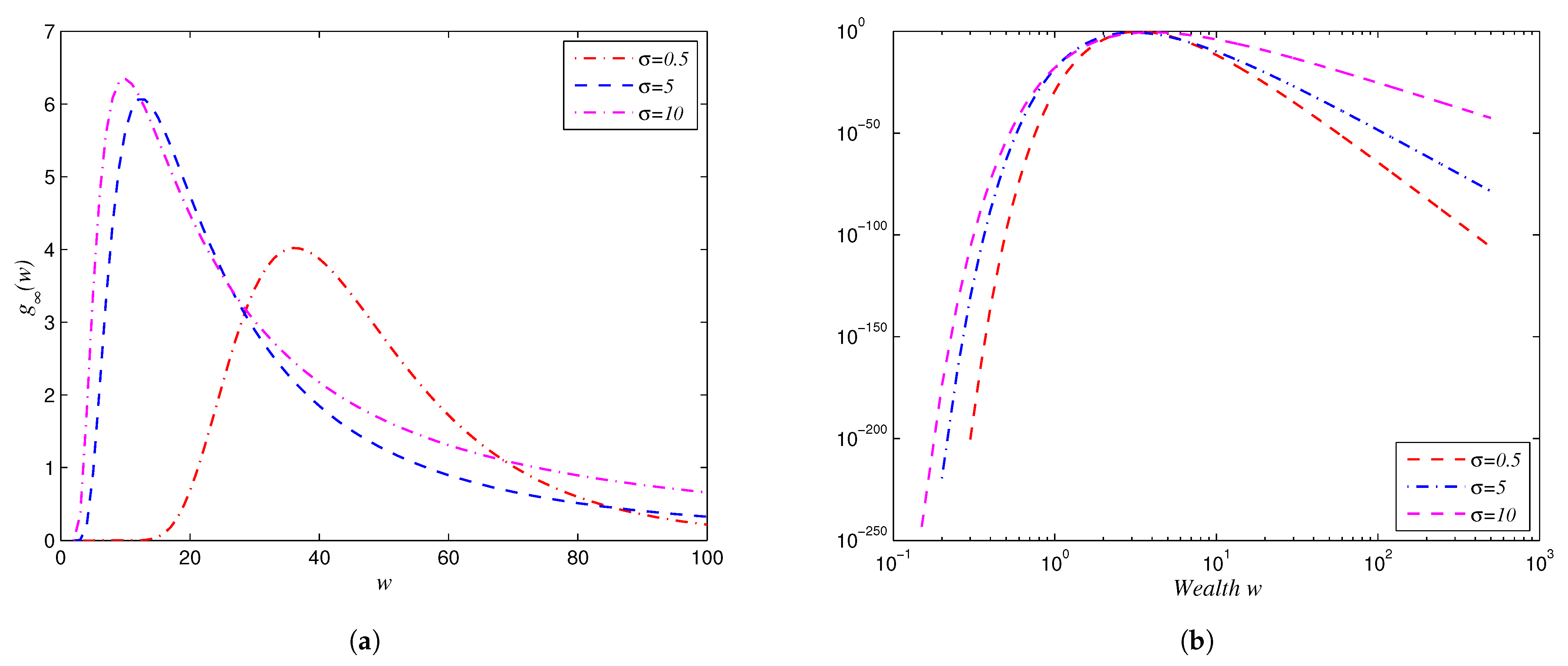
5.1. Is a Decreasing Function About w
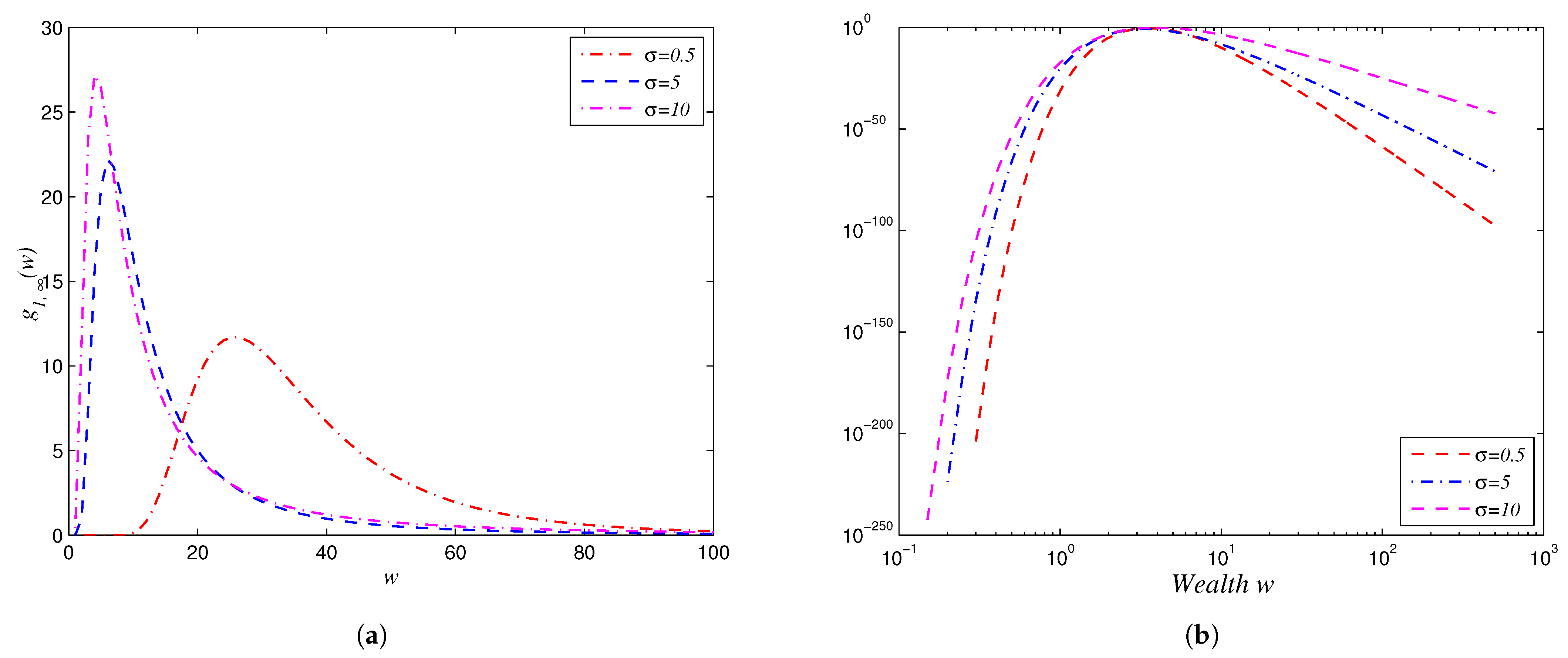
5.2. Is an Increasing Function About w
6. Conclusions
Author Contributions
Funding
Data Availability Statement
Acknowledgments
Conflicts of Interest
References
- Ludwig, D.; Yakovenko, V.M. Physics-inspired analysis of the two-class income distribution in the USA in 1983–2018. Phil. Trans. R. Soc. A 2022, 380, 20210162. [Google Scholar] [CrossRef] [PubMed]
- Düring, B.; Toscani, G. International and domestic trading and wealth distribution. Commun. Math. Sci. 2008, 6, 1043–1058. [Google Scholar] [CrossRef]
- Cordier, S.; Pareschi, L.; Piatecki, C. Mesoscopic modelling of financial markets. J. Stat. Phys. 2009, 134, 161–184. [Google Scholar] [CrossRef]
- Bisi, M.; Spiga, G.; Toscani, G. Kinetic models of conservative economies with wealth redistribution. Commun. Math. Sci. 2009, 7, 901–916. [Google Scholar] [CrossRef]
- Bassetti, F.; Toscani, G. Mean field dynamics of collisional processes with duplication, loss and copy. Math. Model. Methods Appl. Sci. 2015, 25, 1887–1925. [Google Scholar] [CrossRef]
- Bisi, M. Kinetic model for international trade allowing transfer of individuals. Phil. Trans. R. Soc. A 2022, 380, 20210156. [Google Scholar] [CrossRef]
- Maldarella, D.; Pareschi, L. Kinetic models for socio-economic dynamics of speculative markets. Phys. A 2012, 391, 715–730. [Google Scholar] [CrossRef]
- Düring, B.; Pareschi, L.; Toscani, G. Kinetic models for optimal control of wealth inequalities. Eur. Phys. J. B 2018, 91, 265. [Google Scholar] [CrossRef]
- Slanina, F. Inelastically scattering particles and wealth distribution in an open economy. Phys. Rev. E 2004, 69, 046102. [Google Scholar] [CrossRef]
- Goswami, S. A poor agent and subsidy: An investigation through CCM model. Phil. Trans. R. Soc. A 2022, 380, 20210166. [Google Scholar] [CrossRef] [PubMed]
- Toscani, G.; Sen, P.; Biswas, S. Kinetic exchange models of societies and economies. Phil. Trans. R. Soc. A 2022, 380, 20210170. [Google Scholar] [CrossRef]
- Delgadillo-AlemDán, S.E.; Kú-Carrillo, R.A.; Torres-Nájera, A. A corruption impunity model considering anticorruption policies. Math. Comput. Appl. 2024, 29, 81. [Google Scholar]
- Giunta, A.; Giunta, G.; Marino, D.; Oliveri, F. Market behavior and evolution of wealth distribution: A simulation model based on artificial agents. Math. Comput. Appl. 2021, 26, 12. [Google Scholar] [CrossRef]
- Pareto, V. Cours D’economie Politique; Macmillan: Lausanne, Switzerland, 1897. [Google Scholar]
- Pareschi, L.; Toscani, G. Interacting Multiagent Systems: Kinetic Equations and Monte Carlo Methods; Oxford University Press: Oxford, UK, 2013. [Google Scholar]
- Chatterjee, A.; Chakrabarti, B.K.; Manna, S.S. Pareto law in a kinetic model of market with random saving propensity. Phys. Stat. Mech. Its Appl. 2004, 335, 155–163. [Google Scholar] [CrossRef]
- Cordier, S.; Pareschi, L.; Toscani, G. On a kinetic model for a simple market economy. J. Stat. Phys. 2005, 120, 253–277. [Google Scholar] [CrossRef]
- Pareschi, L.; Toscani, G. Wealth distribution and collective knowledge: A Boltzmann approach. Phil. Trans. R. Soc. A 2014, 372, 20130396. [Google Scholar] [CrossRef]
- Bisi, M. Some kinetic models for a market economy. Boll. Unione Mat. Ital. 2017, 10, 143–158. [Google Scholar] [CrossRef]
- Ballante, E.; Bardelli, C.; Zanella, M.; Figini, S.; Toscani, G. Economic segregation under the action of trading uncertainties. Symmetry 2020, 12, 1390. [Google Scholar] [CrossRef]
- Del-Mul, E.M. Kinetic Description of a Market Economy; Politecnico di Milano: Milano, Italy, 2021. [Google Scholar]
- Zhou, X.; Xiang, K.; Sun, R. The study of a wealth distribution model with a linear collision kernel. Math. Probl. Eng. 2021, 2021, 2142876. [Google Scholar] [CrossRef]
- Furioli, G.; Pulvirenti, A.; Terraneo, E.; Toscani, G. Non-Maxwellian kinetic equations modeling the dynamics of wealth distribution. Math. Model. Methods Appl. Sci. 2020, 30, 685–725. [Google Scholar] [CrossRef]
- Düring, D.; Matthes, D.; Toscani, G. A Boltzmann-type approach to the formation of wealth distribution curves. Riv. Mat. Univ. Parma 2009, 8, 199–261. [Google Scholar] [CrossRef]
- Furioli, G.; Pulvirenti, A.; Terraneo, E.; Toscani, G. Fokker–Planck equations in the modelling of socio-economic phenomena. Math. Model. Methods Appl. Sci. 2017, 27, 115–158. [Google Scholar] [CrossRef]


Disclaimer/Publisher’s Note: The statements, opinions and data contained in all publications are solely those of the individual author(s) and contributor(s) and not of MDPI and/or the editor(s). MDPI and/or the editor(s) disclaim responsibility for any injury to people or property resulting from any ideas, methods, instructions or products referred to in the content. |
© 2025 by the authors. Licensee MDPI, Basel, Switzerland. This article is an open access article distributed under the terms and conditions of the Creative Commons Attribution (CC BY) license (https://creativecommons.org/licenses/by/4.0/).
Share and Cite
Liu, Y.; Liu, M.; Lai, S. On the Study of Wealth Distribution with Non-Maxwellian Collision Kernels and Variable Trading Propensity. Math. Comput. Appl. 2025, 30, 63. https://doi.org/10.3390/mca30030063
Liu Y, Liu M, Lai S. On the Study of Wealth Distribution with Non-Maxwellian Collision Kernels and Variable Trading Propensity. Mathematical and Computational Applications. 2025; 30(3):63. https://doi.org/10.3390/mca30030063
Chicago/Turabian StyleLiu, Yaxue, Miao Liu, and Shaoyong Lai. 2025. "On the Study of Wealth Distribution with Non-Maxwellian Collision Kernels and Variable Trading Propensity" Mathematical and Computational Applications 30, no. 3: 63. https://doi.org/10.3390/mca30030063
APA StyleLiu, Y., Liu, M., & Lai, S. (2025). On the Study of Wealth Distribution with Non-Maxwellian Collision Kernels and Variable Trading Propensity. Mathematical and Computational Applications, 30(3), 63. https://doi.org/10.3390/mca30030063