Article

Numerical Simulation of Drilling Fluid-Wellbore Interactions in Permeable and Fractured Zones

by
Diego A. Vargas Silva
1,*,
Zuly H. Calderón
1,
Darwin C. Mateus
2 and
Gustavo E. Ramírez
3
1
Wellbore Stability Research Group, Petroleum Engineering School, Industrial University of Santander, Bucaramanga 680002, Colombia
2
ECOPETROL, Bogotá 681011, Colombia
3
Polymer Research Group, Chemistry Engineering School, Industrial University of Santander, Bucaramanga 680002, Colombia
*
Author to whom correspondence should be addressed.
Math. Comput. Appl. 2025, 30(3), 60; https://doi.org/10.3390/mca30030060
Submission received: 10 April 2025 / Revised: 26 May 2025 / Accepted: 27 May 2025 / Published: 30 May 2025

Abstract

:
In well drilling operations, interactions between drilling fluid water-based and the well-bore present significant challenges, often escalating project costs and timelines. Particularly, fractures (both induced and natural) and permeable zones at the wellbore can result in substantial mud loss or increased filtration. Addressing these challenges, our research introduces a novel coupled numerical model designed to precisely calculate fluid losses in fractured and permeable zones. For the permeable zone, fundamental variables such as filtration velocity, filtrate concentration variations, permeability reduction, and fluid cake growth are calculated, all based on the law of continuity and convection-dispersion theory. For the fracture zone, the fluid velocity profile is determined using the momentum balance equation and both Newtonian and non-Newtonian rheology. The model was validated against laboratory data and physical models, and adapted for field applications. Our findings emphasize that factors like mud particle size, shear stress, and pressure differential are pivotal. Effectively managing these factors can significantly reduce fluid loss and mitigate formation damage caused by fluid invasion. Furthermore, the understanding gathered from studying mud behavior in both permeable and fractured zones equips drilling personnel with valuable information related to the optimal rheological properties according to field conditions. This knowledge is crucial for optimizing mud formulations and strategies, ultimately aiding in the reduction of non-productive time (NPT) associated with wellbore stability issues.

1. Introduction

Fluid losses during drilling operations, a significant challenge in the field, are primarily influenced by mud filtration in permeable areas (at the wellbore and fracture walls) and flow through fractured zones. This phenomenon not only results in fluid losses but also affects other crucial aspects of drilling operations. For instance, changes in filtrate concentration can alter resistivity log readings, impacting data accuracy [1,2,3,4,5]. Furthermore, the rate of mud filtrate advance is known to cause formation damage and contribute to the growth of mud cake, complicating drilling operations [6,7,8,9,10].
The issues analyzed contribute to non-productive time, which costs hundreds of millions of dollars annually and is defined as the time during which the drilling rate is reduced or stopped. States that worldwide, around $20 billion is invested annually in drilling, of which 15% corresponds to NPT. On the other hand, some studies carried out in Colombia in the Castilla field, have shown that lost circulation is the main cause occupying 31% of the NPT [11,12].
The dynamics of mud filtration have been extensively studied both through laboratory experiments and mathematical modeling. Experimental studies focusing on fluid displacement in rock samples have shed light on the impact of mud filtration on formation damage, allowing us to determine the reduction in permeability due to the effect of fluid filtration invasion [13,14,15]. Complementing laboratories are numerical approaches, which have been instrumental in modeling the filtration process and mud cake growth, employing both linear (laboratory) and radial (physical models) coordinates [16,17,18,19]. These models enable the analysis of various interaction scenarios between the drilling fluid and the permeable zone. Proposals in the literature are based on mass balances to determine fluid filtration and fluid concentration changes, studying advective, concentration-gradient, and pressure-gradient transport. Filtrate invasion affects variables such as fluid cake growth, formation permeability, and fluid saturation at the wellbore. This research seeks to couple all of the mentioned phenomena and characterize filtration in a realistic manner.
In naturally fractured zones, the analysis of drilling fluid losses has primarily been based on fluid flow in channels, linking fluid losses to fracture geometry. Some researchers have concentrated on characterizing natural fractures concerning losses observed in the field [20,21], while others have estimated fluid losses based on fracture geometry [22,23,24,25,26,27,28,29,30,31]. Some authors have linked the permeable zone with the fracture zone without including the growth of the fluid cake [24,26,32,33] (Table 1). In addition, sometimes fractures connected by the drilling fluid can reactivate and propagate, which can increase losses, so it is important to strengthen fluid flow and geomechanically couplings (Solid-liquid) [34] and monitor rock properties and stresses over time [35]. The models that analyze fluid losses in fractures have in common that they use the momentum balance equation to propose an expression that relates shear stress to the pressure gradient and then equates it to the rheological model that represents the behavior of the drilling fluid under different shear rates.
In this context, our article introduces a coupled numerical model designed to widely represent the interaction between drilling fluid and the wellbore. This model encompasses the phenomena of mud filtration in permeable zones and fluid flow in natural fractures. For the permeable zone, the mud filtration rate, changes in filtrate concentration, permeability reduction, and mud cake growth were calculated based on the law of continuity and the theory of convection-dispersion. In natural fracture zones, the flow was evaluated, by determining the velocity profile, flow rate, and accumulated volume of losses, using the motion equation balance and incorporating both Newtonian and non-Newtonian rheological models.
This novel modeling approach enhances the precision and understanding of the interaction between drilling fluid and the wellbore. It provides crucial support for decision-making during well-planning and subsequent operational phases.

2. Developed Methodology

Our methodology to analyze the interaction between the drilling fluid and the wellbore through mathematical modeling is divided into two distinct parts, each focusing on different types of zones: permeable and fractured. This structured approach allows for a comprehensive and detailed analysis of each zone type. Figure 1 illustrates the workflow of our methodology.
A.
Analysis of Permeable Zones
In permeable zones, our focus is threefold:
  • Growth of the Mud Cake: Here, we assess the rate and pattern of mud cake formation on the wellbore. This analysis helps in understanding the filtration dynamics and the associated impact on wellbore stability.
  • Filtration Rate: We evaluate the filtration rate of drilling fluid, considering pressure changes at the wellbore. This involves analyzing the pressure differentials and their influence on fluid dynamics and filtration rates.
  • Changes in Filtrate Concentration: This part of the analysis looks at how the filtrate concentration varies over time and its implications for wellbore integrity and drilling efficiency.
B.
Analysis of Fractured Zones
The study of fractured zones involves examining the flow velocity of the drilling fluid, incorporating different rheological models. This segment is further subdivided into:
  • Power Law Velocity: Analysis under this model focuses on the flow behavior of drilling fluids following a Power Law fluid model.
  • Bingham Plastic Velocity: Here, we explore the flow characteristics of drilling fluids modeled as Bingham Plastic fluids, which is crucial for understanding non-Newtonian fluid behavior in fractured zones.
  • Modified Power Law Velocity: This analysis involves a modified approach to the Power Law model, offering insights into complex fluid dynamics in fractured geological structures.

2.1. Numerical Modeling—Permeable Zone

The interaction between the drilling fluid and the permeable zone (Figure 2) depends on the movement of fluids due to the pressure gradient and diffusion due to the concentration gradient. These factors affect the growth of the cake and present the following assumptions.
  • The drilling mud is water-based, and the filtrate exists as a single phase.
  • The properties of the mud cake, such as density and porosity, remain unchanged over time, after the growth of the fluid cake stabilizes over time.
  • The formation is homogeneous, isotropic, and characterized by isothermal flow (This assumption applies to each node in the radial direction, as you move to the next node in the vertical direction, the layer characteristics may change.).
  • Formation properties, are considered constant. (This assumption applies to each node in the radial direction, as you move to the next node in the vertical direction, the layer characteristics may change.).
  • Formation fluid displacement leads to changes in saturation and relative permeabilities.
  • The bottom-hole pressure (pw) is maintained constant (Applies if the density of the drilling fluid remains constant, otherwise the value is updated).
  • The thickness of the cake varies in “r” as a function of time and in the “z” direction as a function of layer properties.
In Section 2.1.1 the proposed mathematical model is derived, based on the assumptions.

2.1.1. Growth of the Mud Cake

The growth of the mud cake is fundamentally driven by the dynamics of particle deposition and erosion in the drilling mud, as outlined in previous studies [17,18,36,37]. It is premised on the assumption that particles suspended in the drilling mud water-based do not displace within the porous medium but only deposit on the wellbore, as expressed in Equation (1).
m c ( k g ) = V c ( 1 c ) ρ c ,
the growth of the fluid cake is determined by the balance between the rates of particle deposition and erosion, as shown in Equation (2):
C a k e   g r o w t h = P a r t i c l e   d e p o s i t i o n P a r t i c l e   e r o s i o n ,
the rate of deposition is defined by Equation (3), and the erosion rate is characterized by Equation (4):
d c = v r C s o l ,
e c = k τ ρ ( 1 )
Literature suggests that the constant k τ is derived from experiments involving latex suspensions (0.04 µm) filtered through glass beads (diameter 0.397 mm and porosity 0.35), using a specific velocity expression to model adhesion and suspension. This results in k τ being defined as k τ = 4.35 × 10 4 s 1 [15,38]. Likewise, the constant k τ has been successfully implemented in previous research [36,37], which used core flooding data to validate your model.
To establish an expression for mass flow per unit of time, Equation (3) is multiplied by the cross-sectional area of filtration, and Equation (4) by the porous volume of the mud cake. These are then substituted into Equation (2), yielding Equation (5):
m t = v r C s o l A k τ ρ ( 1 ) V c ,
Further, by differentiating Equation (1) with respect to time for a radial system and equating it to Equation (5), we derive a new model to determine the growth of the mud cake at the wellbore, as shown in Equation (6). To apply the equation, it is assumed that the properties of the fluid cake such as density and porosity do not change over time
x c t = v r C s o l c 2 r w x c   k τ ρ c ( 1 c ) 2 r w x c x c 2 2 r w x c   ( 1 c ) ρ c ,
where C s o l is the initial concentration, ρ c is the fluid cake density, r w is the wellbore radius, x c is the fluid cake thickness and k τ is the erosion constant and the terms c and v r are the porosity and the filtration rate. The derivation of the equation is seen in Appendix A.

2.1.2. Filtration Rate

In our model, although the bottom hole pressure ( P w ) is considered constant, fluid invasion at the wellbore leads to a pressure increase. To represent this, the continuity equation was used (Equation (7)), which is solved using forward implicit finite differences. To apply the equation, it is assumed that the formation is homogeneous and isotropic, therefore the intrinsic petrophysical properties in the radial direction do not change and as it is assumed isothermal, the viscosity of the filtrate remains constant for the node of study.
1 r d p d r + 2 p r 2 = c r μ k P t ,
where d p d r is the pressure variation between well and reservoir, c r is the compressibility of the rock, μ is the viscosity of the fluid, is the porosity, k is the permeability of the rock, and P t is the pressure variation over time. To analyze the filtration rate in the mud cake, Darcy’s law is applied in radial coordinates, as shown in Equation (8):
v r = k c ( P w P e ) μ r w x c k c k ln re rw + ln r w r w x c ,
where k c is the permeability of the fluid cake, P w P e is the difference between the bottom hole pressure and the reservoir pressure, r w is the radius of the well, x c is the thickness of the fluid cake and r e is the radius of the reservoir affectation.

2.1.3. Concentration of Filtrate

To examine changes in filtrate concentration, we adopt previous research [16,18] which employs the Crank-Nicolson method to approximate and solve the relevant differential equations. The transport of mud particles is analyzed through two primary mechanisms:
Advection Transport: This involves the movement of dissolved solids along with the flowing water, also known as advective transport. The quantity of solute transported depends on its concentration in the water and the volume of water flowing, as expressed in Equation (9) [39]:
C t = v r C r ,
Concentration Gradient Transport: Here, solutes in water migrate from areas of higher concentration to those of lower concentration, a process termed diffusion. This occurs even in static fluid and is governed by Fick’s first law. The mass of fluid diffusing is proportional to the concentration gradient, described by Equation (10) [39]:
C t = D 2 C r 2 + C r r ,
Advective transport is represented by Equation (11) and dispersive transport by Equation (12). The total mass flow is the sum of these two mechanisms, indicated in Equation (13):
A d v e c t i v e   T r a n s p o r t = v r C d A ,
D i s p e r s i v e   T r a n s p o r t = D C r d A
F = v r C D C r
Including Equations (11)–(13) in a mass balance and considering fluid filtration leads to Equation (14):
v r C r + D 2 C r 2 + D r C r = ( C ) t ,
where ( C ) t is the variation in filtrate concentration over time, D is the diffusion constant, and the terms c and v r are the porosity and the filtration rate defined previously. In scenarios with no filtration, movement is solely due to concentration changes, resulting in Equation (15):
D 2 C r 2 + D r C r = ( C ) t ,
For correcting the diffusion coefficient in porous media, we use the correlation D = D i ϵ [40], with exponent values for consolidated formations varying between ϵ = 1.8 to ϵ = 2.
Section 2.1.1, Section 2.1.2 and Section 2.1.3 can also be developed in linear coordinates to validate the phenomenon using laboratory data, as shown in Equations (16) to (18):
m t = v l C s o l A k τ ρ c A x c ( 1 c ) ,
m c t = x c t A ( 1 c ) ρ c
x c t = v l C s o l c k τ ρ ( 1 c ) ) x c   ( 1 c )   ρ c  
For pressure variation, we implement the continuity equation in linear coordinates (Equation (19)):
2 p x 2 = c r μ k P t ,
Flow velocity is estimated using the sample pressure [9], as shown in Equation (20):
v l = k ( P w P o ) μ L k c / k ( k c k + x c ( t ) L ) ,
The concentration of solids at the sample face and for the diffusion coefficient, previous research is used [13,16,17,39], as shown in Equation (21):
D 2 C x 2 + v x C x = ( C ) t ,
Since it is assumed that the displacement of formation fluid leads to changes in saturation and relative permeabilities, it is necessary to calculate their variation in time. Permeability correction due to filtrate invasion is calculated for each time step using the mud saturation equation proposed in previous research [16], as modified in Equation (22):
s m u d = C r C i n i c i a l ( S w m a x S w m i n ) ,
where C r is the filtrate concentration at each distance r , S w m a x S w m i n is the saturation that can change, the difference between the maximum water saturation and the irreducible water saturation, and s m u d represents the increase in filtrate saturation of the fluid that invades the formation. Relative permeability is then calculated using Equation (23) [41]:
k = k r m a x 1 s m u d S w m i n 1 S w m i n   n w ,
For studies lacking documented permeability of the cake, an estimation can be made using the Equation (24) [42]:
k c = r e f 2 e φ t 2 3 δ + 3 δ 5 2 δ 6 3 δ 3 ( 3 + 2 δ 5 ) ,
where r e f is the effective particle radius, φ is the permeability decay constant, γ is the volume fraction of particles in the filter cake, and δ = γ 1 / 3 .

2.2. Numerical Modeling—Fractured Zone

In this part of our study, we focus on the velocity profile of the drilling fluid within fractures (refer to Figure 3). The behavior of the fluid depends on its rheology and the pressure generated by the fluid column. This aspect is approached through the balance of the motion equation [43]. As a result of this balance, a relationship is established between the shear stress perpendicular to the “Z” axis in the “r” direction and the pressure gradient, as shown in Equation (25) (Appendix B).
τ z r = p r z ,
By equating Equation (24) with the rheological model of the fluid, we derive an equation for calculating the velocity profile. This is summarized in Table 2.
Table 2. Velocity Equation Based on Rheological Model.
RheologyEquation
Newtonian v r = p r 1 2 μ w 2 4 z 2 (26)
Power Law v r = p r 1 n n k 1 n n + 1 ( w / 2 ) 1 n + 1 z 1 n + 1 (27)
Bingham Plastic v r = p r 1 2 μ w 2 2 r τ o P 2 + τ o μ r τ o P w 2   i f r < 2 L τ o P (28)
v r = p r 1 2 μ w 2 2 z 2 + τ o μ z w 2   i f r > 2 L τ o P (29)
Plug Flow z = z p and τ o = p r z p
Modified Power Law v r = p r 1 / n 1 1 n + 1 k 1 / n ( ( z z p ) 1 n + 1 w 2 z p 1 n + 1 ) (30)
v r = p r 1 / n 1 1 n + 1 k 1 / n w 2 z p 1 n + 1 (31)
k is the consistency index, w is the fracture width, n is the flow behavior index, p r  is the pressure variation between the fracture and the formation,  τ o  is the initial shear stress used in modified power law and z refers to the fracture width variation.

3. Application of the Numerical Model and Results

The solution of the equations proposed is carried out by means of an algorithm developed in MATLAB-2022. Differential equations whose analytic solution is difficult to implement, are approximated with finite differences using the implicit Crank-Nicolson method (Equation (32)).
2 P x 2 = P i + 1 n + 1 2 P i n + 1 + P i 1 n + 1 r 2 ,   P t = P i n + 1 P i n t ,   P r = P i + 1 n + 1 P i n + 1 r ,
after obtaining the approximations, the matrix is built, for example, the structure for pore pressure would be as follows:
2 A + B + 1 A + B 0 A 2 A + B + 1 A + B 0 A 2 A + B + 1   A P w P i n P i n A + B P o P i n ,
where the constants would group the following properties
c t e = c r μ k ,   A = t c t e r 2 and   B = t c t e r r ,
As for the boundary conditions, there r = r w , p = p w and r = r e , p = p o and for the meshing, similar geometry to the literature models was constructed in order to compare and validate, having a constant radius and angle increment.

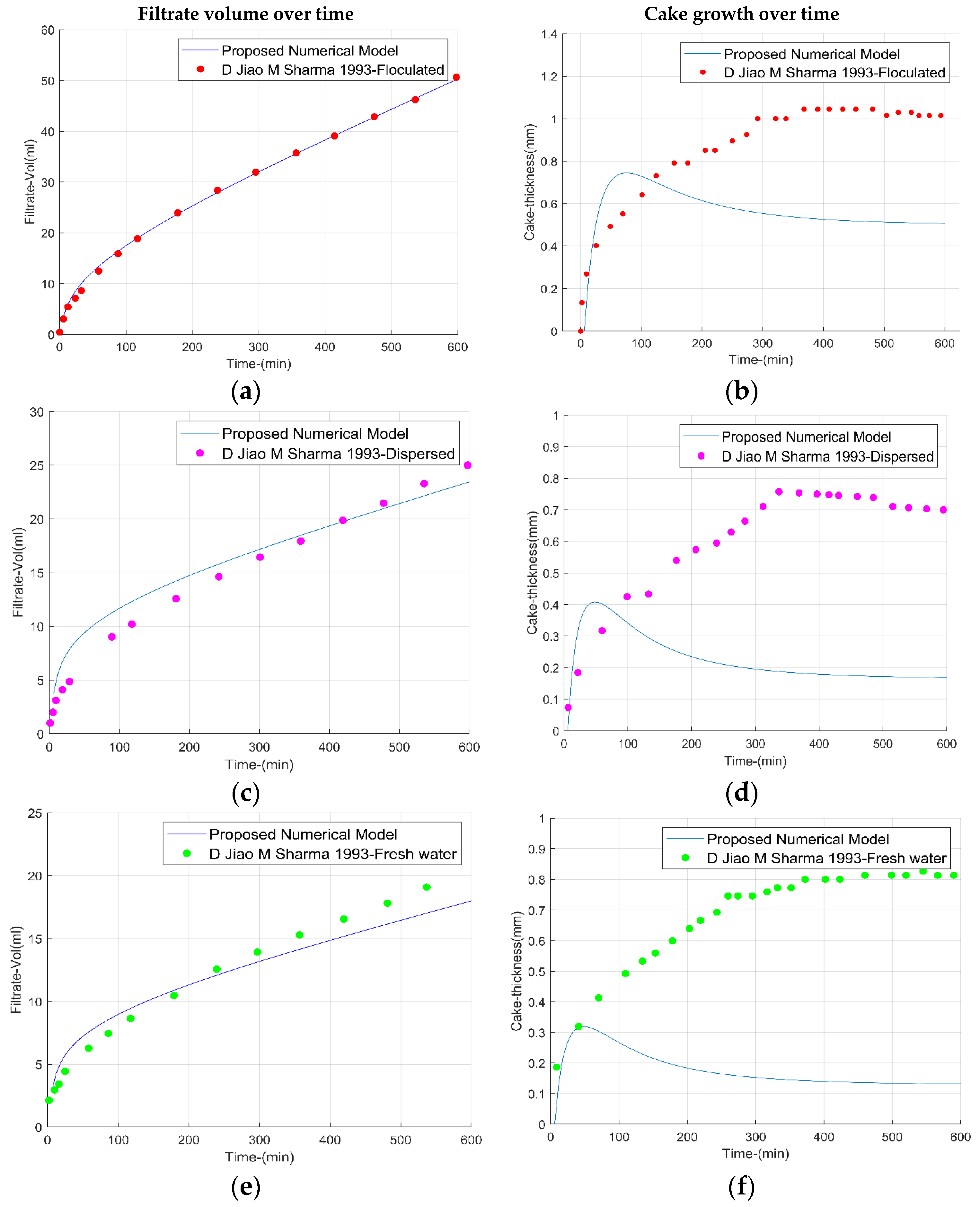
3.1. Interaction with Permeable Zone

For the permeable zone, Ref. [14] analyzed three types of fluids: fresh water, flocculated, and dispersed (Table 3 and Table 4).
To validate our model using data from Table 2 and Table 3, an algorithm was designed in MATLAB, incorporating Equations (16)–(24) in linear coordinates [14].
The accumulated volume of mud filtrate reported in the literature [14] and calculated with our proposed model, exhibits an excellent fit for the three types of fluids, as depicted in Figure 4. However, for cake growth, our model shows a divergence after the initial 50 min, stabilizing at a constant value. This variation appears because the proposed model incorporates the erosion term, unlike the continuous increase reported in the literature [14], which did not consider this factor. The effectiveness of the fluid filter cake growth model was verified by comparing the erosion trend of a physical model published in the literature [44] with the erosion trend generated by Equation (18). In the physical model, upon reaching the maximum thickness, erosion intensifies, decreasing its thickness to a constant thickness as shown by the proposed numerical model.
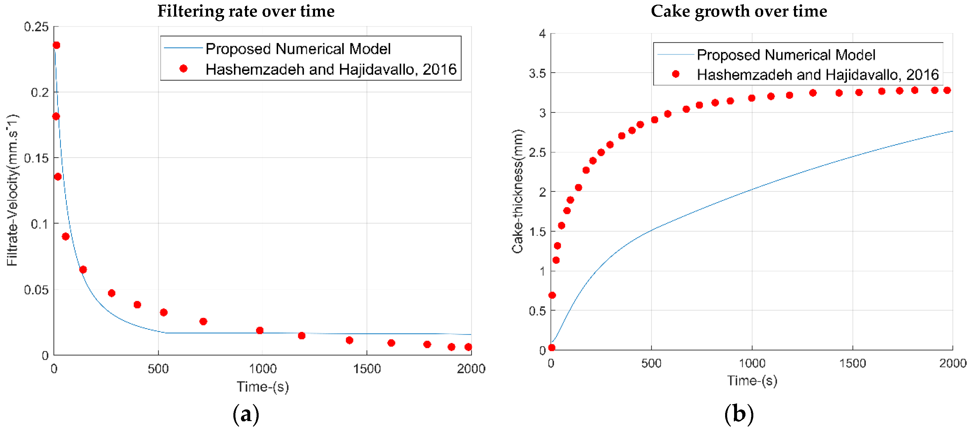
To validate the model for radial coordinates, the data in Table 5 were used [45]. An algorithm was developed in MATLAB, incorporating Equations (6)–(15) and (22)–(24) in radial coordinates. The scenario reported in the literature [45], focusing on the impact of drill string eccentricity and rotational speed on filtrate cake thickness, was used for validation. Their findings indicate that rotational speed does not significantly influence cake size, which corroborates the validity of our base case comparison.
The results for filtration rate and cake growth are shown in Figure 5. Our findings align with literature-reported mud filtration rates, but the cake growth is lower due to the inclusion of the erosion term in our model. By including the erosion term, the fluid cake will grow to a maximum value, and then erosion will intensify until it stabilizes at a constant value.
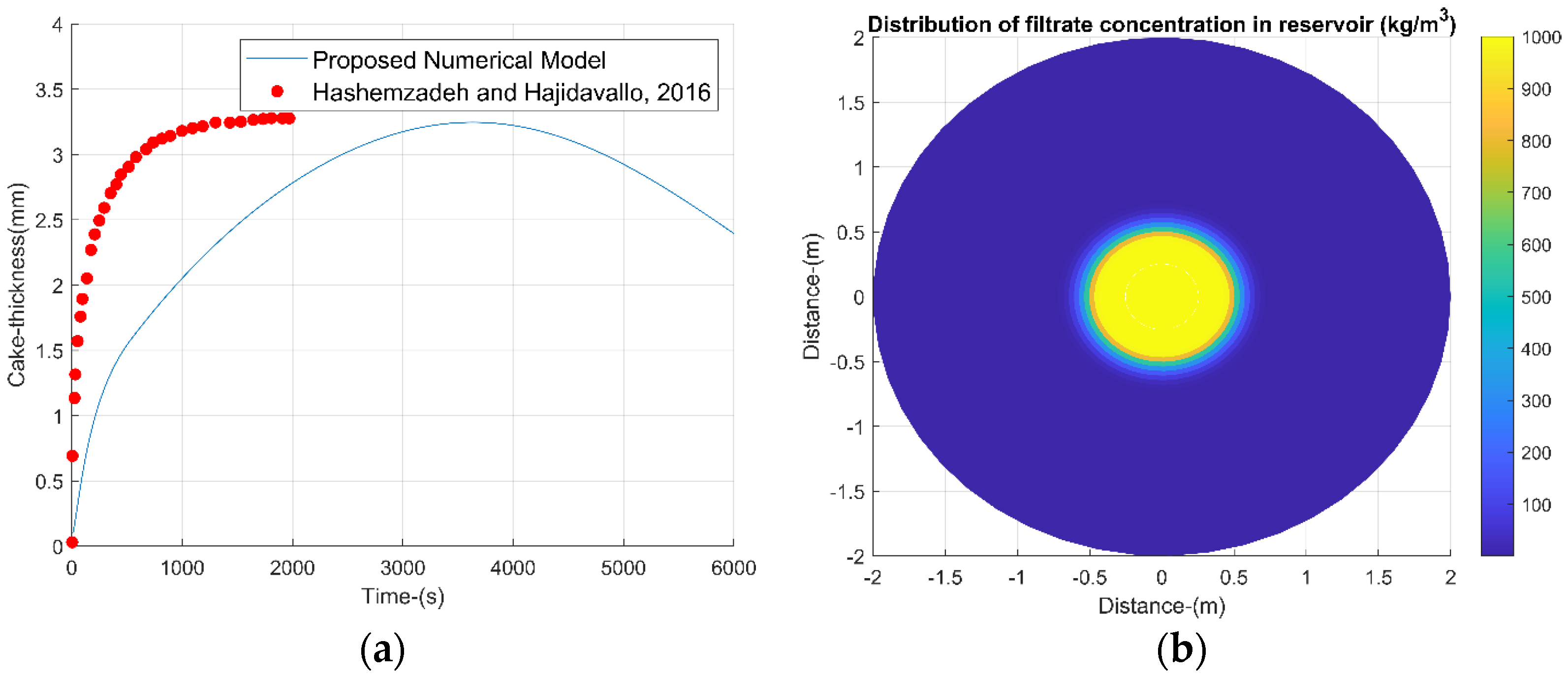
Moreover, the drilling fluid concentration and pore pressure at the wellbore, crucial inputs for Equation (6), were calculated as a function of well radius. This analysis was essential for estimating the invasion radius of the filtrate, which reaches up to 0.5 m, as illustrated in Figure 6. This information is vital for correcting resistivity logs and calculating treatment volumes to mitigate formation damage.

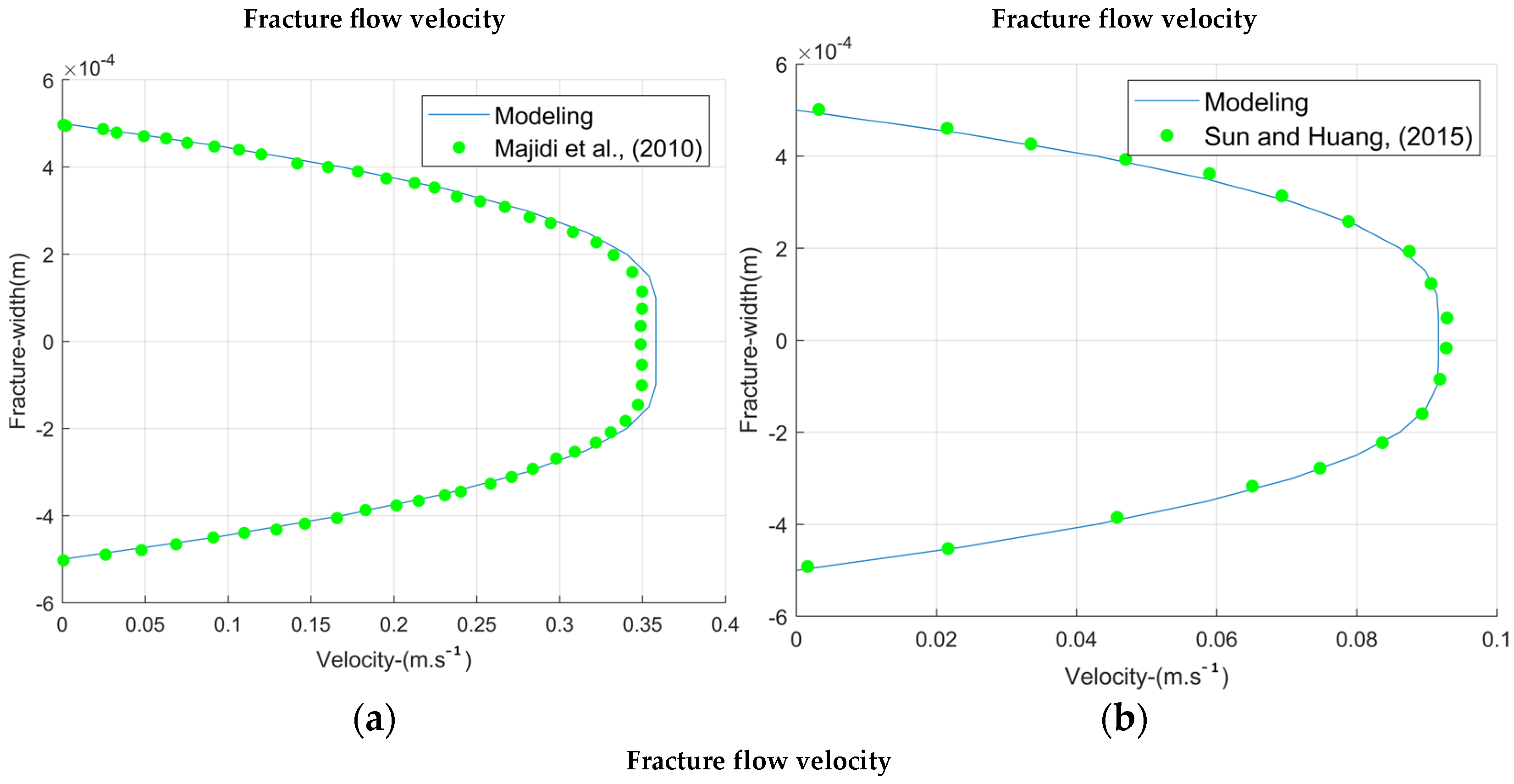
3.2. Interaction with Natural Fractures

To evaluate the interaction between drilling fluid and natural fractures, we applied Equations (26)–(31) suited for different rheological models. The fluid velocity within fractures was calculated based on fracture width and pressure differential. To validate the model with the modified Power Law (Herschel–Bulkley, Equations (30)–(31)) and for the Power Law (Equation (27)). The relevant data for validation is presented in Table 6, and the results of each case are represented in Figure 7.
The validation outcomes with Power Law and modified Power Law models provide credibility to other models based on similar theoretical principles. This suggests that the Bingham Plastic and Newtonian models could also be utilized, contingent upon the specific rheology of the fluid.
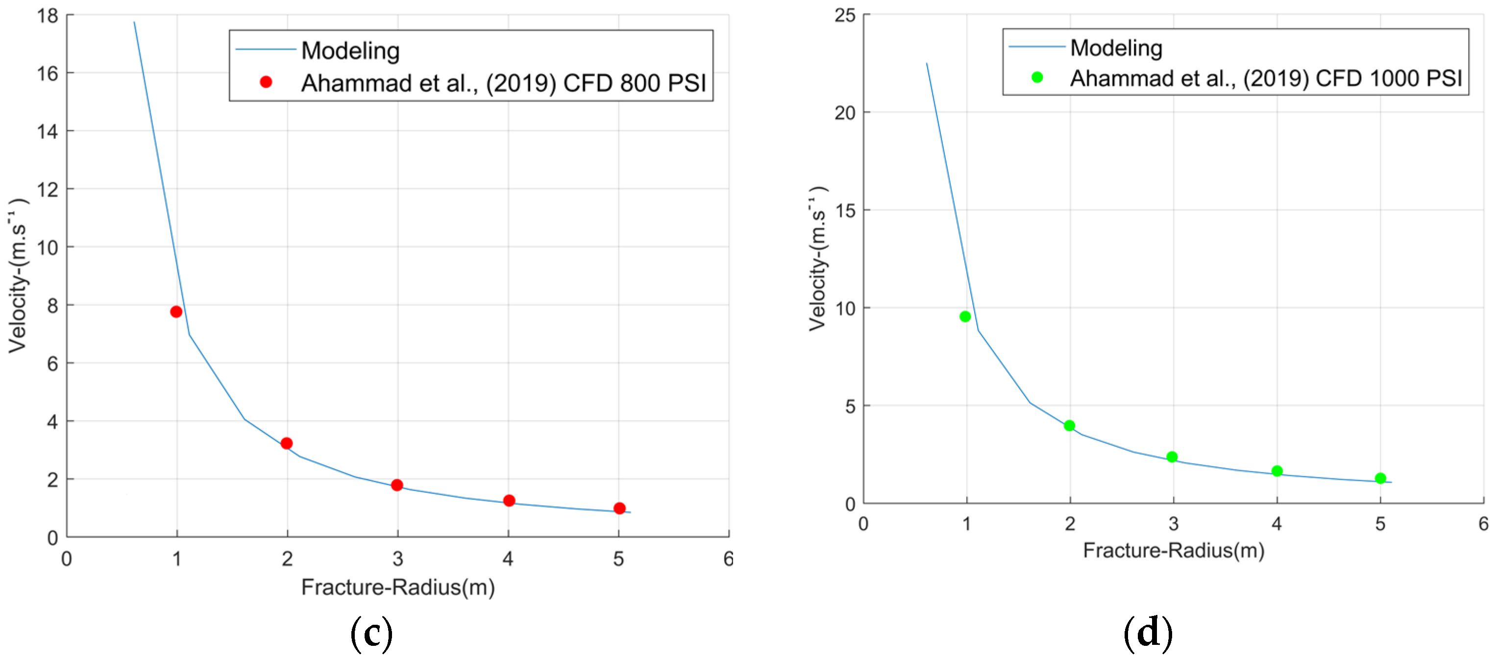
Additionally, to verify the model’s applicability, a comparison was made with a Computational Fluid Dynamics (CFD) study focusing on a horizontal fracture [46]. The data used for this comparison are detailed in Table 7, and the results for scenarios at 200, 500, 800, and 1000 psi are illustrated in Figure 8. The rheology applied in this comparative analysis was Herschel–Bulkley.
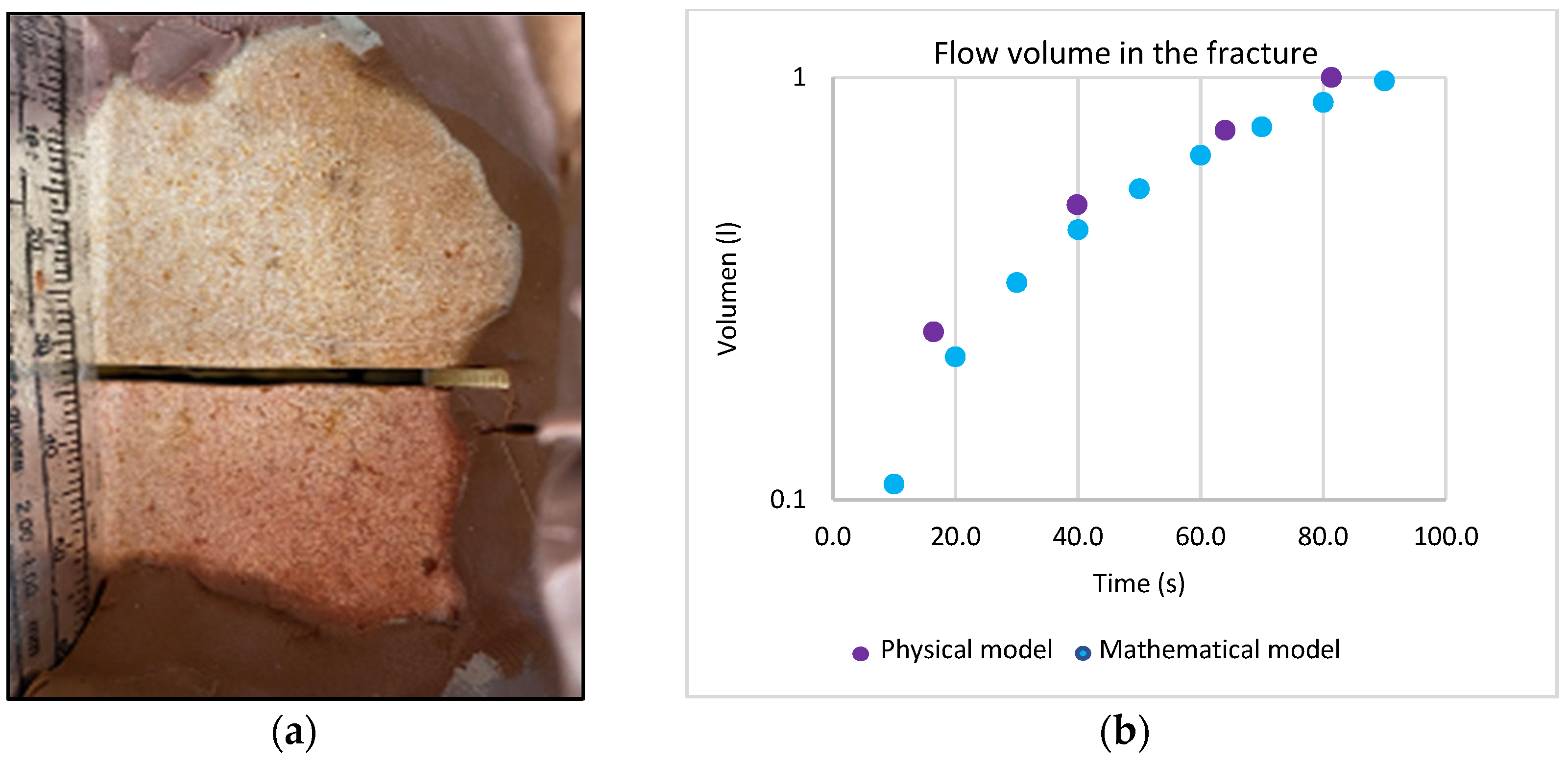
Finally, to confirm the effectiveness of the proposed methodology and before analyzing field data, the results of Equation (27) are compared with the data generated from a physical model [47], which consists of measuring the time it takes for a liter of drilling fluid to flow through a fracture with known dimensions. The fracture and the comparison of results are shown in Figure 9.

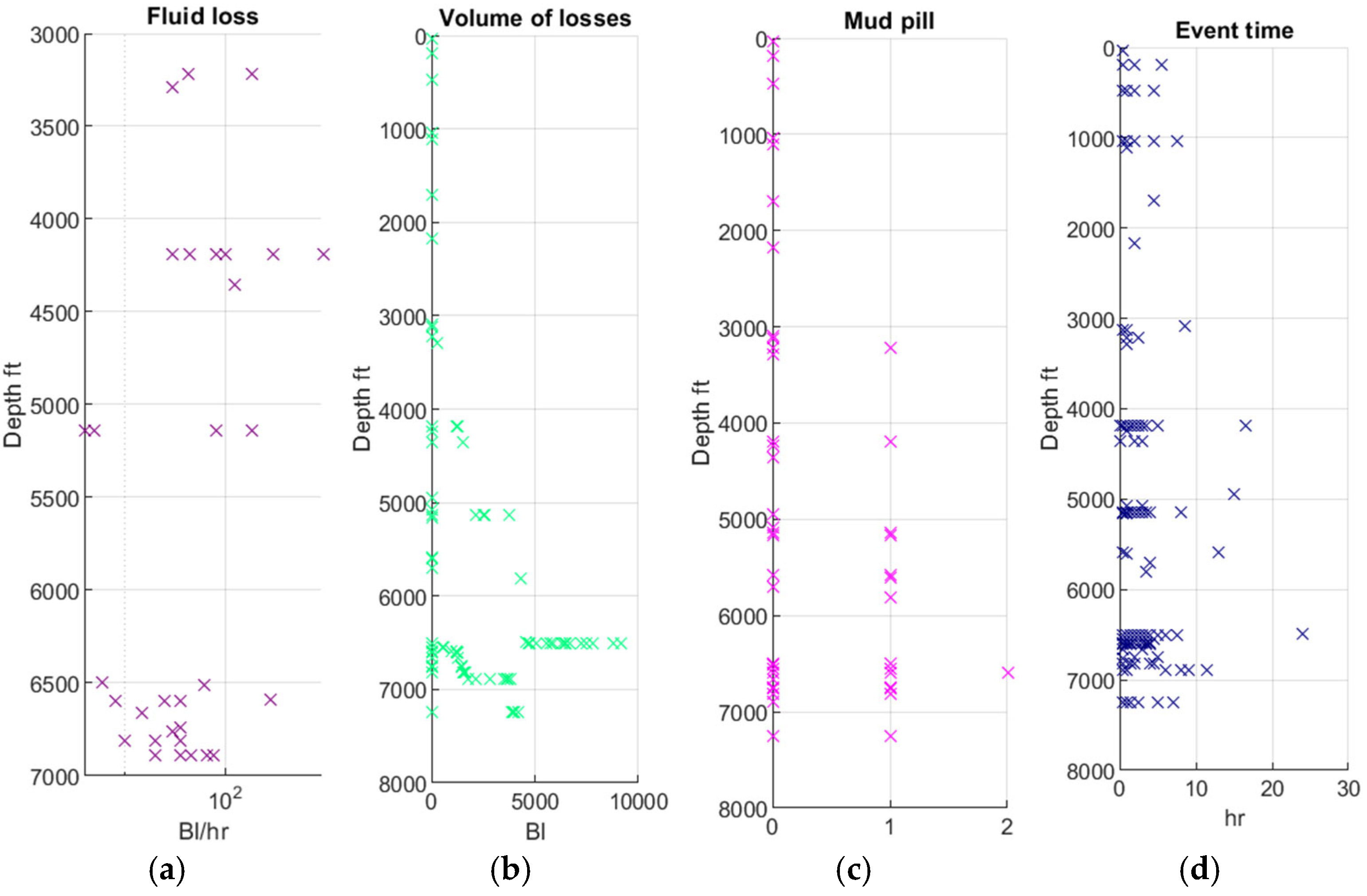
4. Field Application

After implementing the numerical model and validating it with data from the literature, the next step is to carry out an application in a Colombian field, estimating the rate of drilling fluid losses in fracture zones and filtrate in the permeable zone. The field of study is the Llanos Orientales basin. For the application, the GeoDrill-Flow tool was developed using MATLAB’s APPDESIGNER, which is an interactive development environment that facilitates the design of applications and the programming of their behavior. The information required for the application is loss events, fracture geometry (inclination and azimuth), geomechanical model, petrophysical model, mud weight, bit position, and mud rheology, as shown in Figure 10, Figure 11 and Figure 12. In addition to the information mentioned, the data in Table 8 is required [48].
With the field information and the model developed in Section 2, we proceed to estimate the growth of the fluid cake, the filtration rate, the velocity of fluid losses, the permeability of the fluid cake, the pressure changes, and the concentration changes as observed in Figure 13.
The variables calculated in Figure 13 allow us to determine the pressure variation within the fracture (Figure 14a) and total fluid loss rate (Figure 14b), including the flow in the fracture and the filtrate in the permeable zone, which is compared with field data.
Figure 14b is applied to a drill bit diameter 12 ¼ in to a depth of around 6500 ft. From that section on, the diameter changes, so another modeling would have to be performed. This figure shows an excellent fit between field data and modeled data, which highlights the effectiveness of the coupled model implemented.

5. Discussion

The developed model facilitates a comprehensive analysis of the interaction between drilling fluid and the permeable zone, accounting for variables such as petrophysics, rheology, and operational conditions. Additionally, the model assesses the impact of the mud’s exposure time on the wellbore, which is crucial for understanding cake growth dynamics. This aspect is particularly relevant in field operations, where the well remains exposed to the mud until casing placement. For prolonged exposure periods, our model determines the maximum cake growth value, as illustrated in Figure 15a. Furthermore, recording the filtrate invasion radius (Figure 15b) is essential to comprehend the extent of the invaded zone and to strategize cleaning treatment volumes, therefore minimizing formation damage.
In Figure 16, the maximum thickness observed in the mud cake is approximately 3 mm. This value is lower than the thickness reported in previous research [45], which can be attributed to the erosion factor included in our model. Regarding the invasion radius, it extends to 0.6 m, 20% deeper than indicated in Figure 6. This expansion is due to the longer study duration, suggesting that prolonged mud exposure leads to a larger affected radius, independent of pressure differential. The filtrate movement can occur due to concentration changes.
Another critical aspect is the size of the mud particles, which significantly influences permeability reduction, mud cake growth, and filtrate invasion. For instance, Figure 16 demonstrates the permeability reduction as a function of particle size. Smaller particles result in lower permeability and thinner mud cakes, which are advantageous in drilling operations.
As indicated in Figure 8, an increase in fracture radius leads to a decrease in fluid velocity. This observation can be combined with other variables to mitigate fluid losses. For example, a similar trend is evident when pressure decreases (Figure 17a) and with varying initial shear stress levels (Figure 17b). Higher initial stress slows down fluid movement, suggesting that fluids with high yield stress can help decrease losses. Similarly, smaller particles improve the mud cake quality, reducing filtrate invasion.

6. Conclusions

This study introduces a comprehensive methodology to improve the interaction between drilling fluid and the wellbore. It effectively estimates fluid velocity within fractures in naturally fractured reservoirs, and examines the influence of rheology, pressure, and operational conditions on this interaction.
Key contributions of the proposed model include:
  • Analysis of Fluid-Wellbore Interactions: The model offers insights into the dynamics between drilling fluid and wellbore, analyzing the permeable and fracture zone, and factoring in petrophysical properties, fluid rheology, and operational conditions.
  • Impact of Mud Exposure Time: It highlights the significance of mud exposure time on the wellbore, a critical aspect in field operations where the well is exposed until casing placement. This feature of the model is vital for understanding the implications of prolonged mud exposure.
  • Quantification of Drilling Dynamics: Through the coupled model, we quantitatively evaluate various factors such as filtration velocity, filtrate concentration, filter cake formation, and invasion radius. This approach incorporates time and distance-based analysis and applies convection-dispersion theory to explore different mass transfer mechanisms in permeable zones.
  • Informing Operational Decisions: The understanding gathered from studying mud behavior in both permeable and fractured zones equips drilling and mud personnel with valuable information. This knowledge is crucial for optimizing mud formulations and strategies, ultimately aiding in the reduction of non-productive time (NPT) associated with wellbore stability issues.
In summary, the proposed model enhances the understanding of complex fluid dynamics within wellbores, thereby contributing to more efficient and effective drilling operations, particularly in challenging geological settings.

Author Contributions

Conceptualization, methodology, software, D.A.V.S.; validation, D.A.V.S., D.C.M. and Z.H.C.; formal analysis, D.A.V.S.; investigation, D.A.V.S. and Z.H.C.; resources, D.A.V.S.; data curation, D.C.M.; writing—original draft preparation, D.A.V.S.; writing—review and editing, Z.H.C. and G.E.R.; visualization, Z.H.C. and G.E.R.; supervision, Z.H.C. and D.C.M.; project administration, D.A.V.S.; funding acquisition, (no funding was received). All authors have read and agreed to the published version of the manuscript.

Funding

This research received no external funding.

Data Availability Statement

The data previously published in the master’s thesis https://noesis.uis.edu.co/handle/20.500.14071/37566 (1 January2022).

Acknowledgments

Thanks to the Well Stability Research Group (GIEP) for their advice.

Conflicts of Interest

The authors declare no conflicts of interest.

Nomenclature

The following nomenclature is used in this paper, with units provided for clarity:
TermNomenclatureUnits *
V c Cake volume m 3
m c Cake mass k g
c Cake porosity
k d Deposition constant s 1
k τ Erosion constant s 1
d c Deposition rate k g / s
e c Erosion rate k g / s
C s o l Filtrate concentration k g / m 3
v r   v l Filtration velocity m / s
ACross-sectional area m 2
m t Mass flow rate k g / s
x c Cake thickness m
c r Rock compressibility 1 / P a
μ Fluid viscosity P a s
k Fluid permeability m 2
Formation porosity
P w P e Bottom hole and reservoir pressures P a
k c Cake permeability m 2
r w Well radius m
x c Cake thickness m
D Diffusion coefficient m 2 / s
L Sample length c m
r e f Effective particle radiusmm
φ Permeability decay constantDimensionless
δ = γ 1 / 3 γ is the volume fraction of particles in the filter cakeDimensionless
K Consistency index P a s n
n Flow behavior indexDimensionless
τ o Initial yield stress P a
w Fracture width m
* Note: For equations in linear coordinates, the cgs system is used.

Appendix A. Fluid Cake Growth

Starting from a mass balance we have
m c t = t V c ( 1 c ) ρ c
replacing V c by π r w 2 π ( r w x c ) 2 h
m c t = t π r w 2 π ( r w x c ) 2   h ( 1 c ) ρ c
Solving and simplifying ( r w x c ) 2
m c t = t π r w 2 π ( r w 2 2 r w x c + x c 2 ) h ( 1 c ) ρ c
m c t = t 2 π r w x c π   x c 2 h ( 1 c ) ρ c
Applying the derivative and factoring,
m c t = 2 π r w x c t 2 π   x c x c t h ( 1 c ) ρ c
m c t = 2 π r w x c   x c t h ( 1 c ) ρ c
Remembering the Equation (5),
m t = v r C s o l c A k τ ρ V c
Equating the Equations (A6) and (A7), the following expression is obtained,
2 π r w x c   x c t h 1 c ρ c = v r C s o l c A k τ ρ V c
Knowing that the volume of the cake is 2 π r w x c π x c 2 h ( 1 c ) , V c is replaced,
2 π r w x c   x c t h 1 c ρ c = v r C s o l c 2 π r w x c   h k τ ρ c 2 π r w x c π   x c 2 h 1 c
Simplifying π h , the expression to calculate the fluid cake growth is found.
x c t = v r C s o l c 2 r w x c   k τ ρ c ( 1 c ) 2 r w x c x c 2 2 r w x c   ( 1 c ) ρ c

Appendix B. Balance of the Equation of Motion

ρ v r t + v r v r r + v θ r v r θ + v z v r z v θ 2 r = p r 1 r ( r τ r r ) r + 1 r τ θ r θ + τ z r z τ θ θ r + ρ g r ρ v θ t + v r v θ r + v θ r v θ θ + v z v θ z v r v θ r = 1 r p θ 1 r 2 ( r 2 τ r θ ) r + 1 r τ θ θ θ + τ z θ z τ θ r τ r θ r + ρ g θ ρ v z t + v r v z r + v θ r v z θ + v z v z z = p z 1 r ( r τ r z ) r + 1 r τ θ z θ + τ z z z + ρ g z
Taking the radial component (Equation (A11))
ρ v r t + v r v r r + v θ r v r θ + v z v r z v θ 2 r = p r 1 r ( r τ r r ) r + 1 r τ θ r θ + τ z r z τ θ θ r + ρ g r
Knowing that, v r = v r ( z ) , v z = 0 ,   v θ = 0 and p = p ( z ) , Equation (A12) reduces to Equation (A14)
0 = p r τ z r z
τ z r z = p r  
Integrating we have
τ z r = p r z + c
Considering z = 0 and τ z r = 0 , therefore the constant c = 0
τ z r = p r z

References

  1. Semmelbeck, M.E.; Holditch, S.A. Effects of mud-filtrate invasion on the interpretation of induction logs. SPE Form. Eval. 1988, 3, 386–392. [Google Scholar] [CrossRef]
  2. Lane, H.R. Numerical simulation of mud filtrate invasion and dissipation. In Proceedings of the SPWLA 34th Annual Logging Symposium, Calgary, AB, Canada, 13–16 June 1993. [Google Scholar]
  3. Wu, J.; Torres-Verdín, C.; Sepehrnoori, K.; Delshad, M. Numerical simulation of mud filtrate invasion in deviated wells. In Proceedings of the SPE Annual Technical Conference and Exhibition, Orleans, LA, USA, 30 September–3 October 2001; pp. 3701–3715, Society of Petroleum Engineers. [Google Scholar] [CrossRef]
  4. Chowdhury, S.; Torres-Verdín, C.; Mezzatesta, A. Interpretation of borehole measurements acquired in laminated clastic sequences subject to mud-filtrate invasion. In Proceedings of the SPE Annual Technical Conference and Exhibition, Houston, TX, USA, 26–29 September 2004. Society of Petroleum Engineers. [Google Scholar] [CrossRef]
  5. Jiang, Y.; Sun, J.; Gao, J.; Cui, J. Mud invasion and array laterolog responses in horizontal well based on numerical simulation. J. Geophys. Eng. 2017, 14, 15–25. [Google Scholar] [CrossRef]
  6. Dewan, J.T.; Chenevert, M.E. A model for filtration of water-base mud during drilling: Determination of mudcake parameters. Petrophysics 2001, 42, 237–250. [Google Scholar]
  7. Amanullah, M. A novel laboratory method for assessing the erosional characteristics of mudcakes. In Proceedings of the SPE/IADC Drilling Conference, Abu Dhabi, United Arab Emirates, 20–22 October 2003; pp. 411–420, Society of Petroleum Engineers. [Google Scholar] [CrossRef]
  8. Calçada, L.; Scheid, C.; de Araújo, C.; Waldmann, A.; Martins, A. Analysis of dynamic and static filtration and determination of mud cake parameters. Braz. J. Pet. Gas 2011, 5, 159–170. [Google Scholar] [CrossRef]
  9. Khalid, M. Investigating the Effect of Fluid and Formation Parameters on Mud Cake Thickness, Filtration Velocity and Invasion Depth. ResearchGate 2016; Department of Geoscience & Petroleum Engineering Universiti Teknologi PETRONAS, Malaysia. Available online: https://www.researchgate.net/publication/311304765_Investigating_the_Effect_of_Fluid_and_Formation_Parameters_on_Mud_Cake_Thickness_Filtration_Velocity_and_Invasion_Depth?channel=doi&linkId=5841210908ae8e63e6213cf2&showFulltext=true (accessed on 1 January 2023).
  10. Adewole, J.K.; Kazeem, T.S.; Oyehan, T.A. Molecular transport of solutes and ions through filter-cake: Implications for wellbore instability and formation damage. In Proceedings of the SPE Kingdom of Saudi Arabia Annual Technical Symposium and Exhibition 2018, Dammam, Saudi Arabia, 23–26 April 2018. Society of Petroleum Engineers. [Google Scholar] [CrossRef]
  11. Moazzeni, A.R.; Nabaei, M.; Ghadami, S. Nonproductive time reduction through a deep-rig time analysis: Case study. In Proceedings of the SPE Digital Energy Conference and Exhibition, The Woodlands, TX, USA, 19–21 April 2011; p. SPE–142799, SPE. [Google Scholar] [CrossRef]
  12. Emhana, S. Analysis of non-productive time (NPT) in drilling operations—A case study of the Ghadames Basin. In Proceedings of the Second Scientific Conference of Oil and Gas, Ajdabiya, Libya, 5–7 February 2018; pp. 5–7. [Google Scholar]
  13. Donaldson, E.C.; Chernoglazov, V. Characterization of drilling mud fluid invasion. J. Pet. Sci. Eng. 1987, 1, 3–13. [Google Scholar] [CrossRef]
  14. Jiao, D.; Sharma, M. Mechanism of cake buildup in crossflow filtration of colloidal suspensions. J. Colloid Interface Sci. 1993, 169, 264–270. [Google Scholar] [CrossRef]
  15. Corapcioglu, M.Y.; Abboud, N.; Haridas, A. Governing equations for particle transport in porous media. In Advances in Transport Phenomena in Porous Media; Springer: Berlin/Heidelberg, Germany, 1987; pp. 269–342. [Google Scholar] [CrossRef]
  16. Civan, F.; Engler, T. Drilling mud filtrate invasion—Improved model and solution. J. Pet. Sci. Eng. 1994, 11, 183–193. [Google Scholar] [CrossRef]
  17. Liu, X.; Civan, F. Formation damage and filter cake buildup in laboratory core tests: Modeling and model-assisted analysis. SPE Form. Eval. 1996, 11, 26–30. [Google Scholar] [CrossRef]
  18. Parn-Anurak, S.; Engler, T.W. Modeling of fluid filtration and near-wellbore damage along a horizontal well. J. Pet. Sci. Eng. 2005, 46, 149–160. [Google Scholar] [CrossRef]
  19. Shad, S.; Salmanpour, S.; Zamani, H.; Zivar, D. Dynamic analysis of mud loss during overbalanced drilling operation: An experimental study. J. Pet. Sci. Eng. 2021, 196, 107984. [Google Scholar] [CrossRef]
  20. Sanfillippo, F.; Brignoli, M.; Santarelli, F.; Bezzola, C. Characterization of conductive fractures while drilling. In Proceedings of the SPE European Formation Damage Conference and Exhibition, The Hague, The Netherlands, 2–3 June 1997; p. SPE–38177, Society of Petroleum Engineers. [Google Scholar] [CrossRef]
  21. Liétard, O.; Unwin, T.; Guillo, D.J.; Hodder, M.H. Fracture width logging while drilling and drilling mud/loss-circulation-material selection guidelines in naturally fractured reservoirs. SPE Drill. Complet. 1999, 14, 168–177. [Google Scholar] [CrossRef]
  22. Lavrov, A.; Tronvoll, J. Modeling mud loss in fractured formations. In Proceedings of the Abu Dhabi International Petroleum Exhibition and Conference, Abu Dhabi, United Arab Emirates, 10–13 October 2004; p. SPE–88700, Society of Petroleum Engineers. [Google Scholar] [CrossRef]
  23. Lavrov, A.; Tronvoll, J. Mechanics of borehole ballooning in naturally-fractured formations. In Proceedings of the SPE Middle East Oil and Gas Show and Conference, Kingdom of Bahrain, 12–15 March 2005; p. SPE–93747, Society of Petroleum Engineers. [Google Scholar] [CrossRef]
  24. Xia, Y.; Jin, Y.; Chen, M.; Chen, K.P.; Lin, B.T.; Hou, B. Hydrodynamic modeling of mud loss controlled by the coupling of discrete fracture and matrix. J. Pet. Sci. Eng. 2015, 129, 254–267. [Google Scholar] [CrossRef]
  25. Xia, Y.; Jin, Y.; Chen, M. Comprehensive methodology for detecting fracture aperture in naturally fractured formations using mud loss data. J. Pet. Sci. Eng. 2015, 135, 515–530. [Google Scholar] [CrossRef]
  26. Vargas, D.; Calderon, Z.; Mateus, D. Assessment of the drilling fluid losses phenomenon in naturally-fractured reservoir by numerical modeling that couples fracture plane and permeable zone. In Proceedings of the ISRM 8th International Symposium Geomechanics, Bucaramanga, Colombia, 6–10 May 2019; pp. 978–981. [Google Scholar]
  27. Majidi, R.; Miska, S.Z.; Ahmed, R.; Yu, M.; Thompson, L.G. Radial flow of yield-power-law fluids: Numerical analysis, experimental study, and the application for drilling fluid losses in fractured formations. J. Pet. Sci. Eng. 2010, 70, 334–343. [Google Scholar] [CrossRef]
  28. Sun, Y.; Huang, H. Effect of rheology on drilling mud loss in a natural fracture. In Proceedings of the 49th US Rock Mechanics/Geomechanics Symposium, San Francisco, CA, USA, 28 June–1 July 2015; Volume 4, pp. 2678–2684. [Google Scholar]
  29. Shahri, P.; Zeyghami, M.; Majidi, R. Investigation of fracture ballooning and breathing in naturally fractured reservoirs: Effect of fracture deformation law. In Proceedings of the Nigeria Annual International Conference and Exhibition, Abuja, Nigeria, 30 July–3 August 2011. OnePetro. [Google Scholar] [CrossRef]
  30. Shahri, P.; Mehrabi, M. A new approach in modeling of fracture ballooning in naturally fractured reservoirs. In Proceedings of the SPE Kuwait International Petroleum Conference and Exhibition, Kuwait City, Kuwait, 10–12 December 2012. OnePetro. [Google Scholar] [CrossRef]
  31. Lavrov, A. Flow of truncated power-law fluid between parallel walls for hydraulic fracturing applications. J. Non-Newton. Fluid Mech. 2015, 223, 141–146. [Google Scholar] [CrossRef]
  32. Bychina, M.; Thomas, G.M.; Khandelwal, R.; Samuel, R. A robust model to estimate the mud loss into naturally fractured formations. In Proceedings of the SPE Annual Technical Conference and Exhibition, San Antonio, TX, USA, 9–11 October 2017; p. D011S005R008, SPE. [Google Scholar] [CrossRef]
  33. Bao, K.; Lavrov, A.; Nilsen, H. Numerical modelling of non-Newtonian fluid flow in fractures and porous media. In Proceedings of the ECMOR XV-15th European Conference on the Mathematics of Oil Recovery, Amsterdam, The Netherlands, 29 August–1 September 2016; p. cp–494, European Association of Geoscientists & Engineers. [Google Scholar] [CrossRef]
  34. Li, Q.; Li, Q.; Cao, H.; Wu, J.; Wang, F.; Wang, Y. The crack propagation behaviour of CO2 fracturing fluid in unconventional low permeability reservoirs: Factor analysis and mechanism revelation. Processes 2025, 13, 159. [Google Scholar] [CrossRef]
  35. Li, Q.; Li, Q.; Wu, J.; Li, X.; Li, H.; Cheng, Y. Wellhead stability during the development process of hydrate reservoir in the Northern South China Sea: Evolution and mechanism. Processes 2024, 13, 40. [Google Scholar] [CrossRef]
  36. Windarto, G.; Sukarno, P.; Soewono, E. Modeling of mud filtrate invasion and damage zone formation. J. Pet. Sci. Eng. 2011, 77, 359–364. [Google Scholar] [CrossRef]
  37. Windarto, G.; Sukarno, P.; Soewono, E. Modelling of formation damage due to mud filtrate invasion in a radial flow system. J. Pet. Sci. Eng. 2012, 100, 99–105. [Google Scholar] [CrossRef]
  38. Ring, T. Bed filtration of colloidal particles. Prepr. Soc. Min. Eng. AIME 1983, 276, 1838–1842. [Google Scholar]
  39. Fetter, C.; Boving, T.; Kreamer, D. Contaminant hydrogeology. In Contaminant hydrogeology; Waveland Press: Long Grove, IL, USA, 2017. [Google Scholar] [CrossRef]
  40. Coutelieris, F.; Delgado, J. Advanced Structured Materials: Transport Processes in Porous Media; Springer: Berlin/Heidelberg, Germany, 2012; Volume 20. [Google Scholar]
  41. Proett, M.A.; Chin, W.; Wu, J.; Manohar, M.; Belanger, D. Sample quality prediction with integrated oil and water-based mud invasion modeling. In Proceedings of the SPE—Asia Pacific Oil and Gas Conference, Melbourne, Australia, 8–10 October 2002; pp. 1081–1094. [Google Scholar] [CrossRef]
  42. Fisher, K.; Wakeman, R.; Chiu, T.; Meuric, O. Numerical modelling of cake formation and fluid loss from non-Newtonian muds during drilling using eccentric/concentric drill strings with/without rotation. Chem. Eng. Res. Des. 2000, 78, 707–714. [Google Scholar] [CrossRef]
  43. Byron, B. Fenómenos de Transporte, 2nd ed.; Wikipedia: San Francisco, CA, USA, 2006; Volume 2. [Google Scholar]
  44. van Opedal, N.; Cerasi, P.; Ytrehus, J.D. Dynamic fluid erosion on filter cakes. In Proceedings of the SPE European Formation Damage Conference and Exhibition, Noordwijk, The Netherlands, 5–7 June 2013; p. SPE–165107, SPE. [Google Scholar] [CrossRef]
  45. Hashemzadeh, S.M.; Hajidavalloo, E. Numerical investigation of filter cake formation during concentric/eccentric drilling. J. Pet. Sci. Eng. 2016, 145, 161–167. [Google Scholar] [CrossRef]
  46. Ahammad, F.; Mahmud, S.; Islam, S. Computational fluid dynamics study of yield power law drilling fluid flow through smooth-walled fractures. J. Pet. Explor. Prod. Technol. 2019, 9, 2717–2727. [Google Scholar] [CrossRef]
  47. Vargas, D.; Uribe, L.; Calderón, Z.; Bernal, R. Estimación de pérdidas de lodo a través de fracturas mediante modelamiento matemático y su validación mediante un modelo físico. Boletín De Geol. 2024, 46, 103–114. [Google Scholar] [CrossRef]
  48. Vargas, D. Modelamiento Numérico de Pérdidas de Fluido de Perforación En Zonas Fracturadas; Universidad Industrial de Santander: Bucaramanga, Colombia, 2017; Available online: https://noesis.uis.edu.co/handle/20.500.14071/37566 (accessed on 1 January 2023).
Figure 1. Workflow to Analyze the Interaction Between Drilling Fluid and Wellbore.
Mca 30 00060 g001
Figure 2. Radial Geometry with Side and Top View of the interaction between the drilling fluid and the permeable zone.
Mca 30 00060 g002
Figure 3. Velocity Profile of Drilling Fluid Within the Fracture.
Mca 30 00060 g003
Figure 4. Comparison of Filtration Rate and Cake Growth for Different Fluids; (a,b) for flocculated; (c,d) for dispersed and (e,f) for fresh water [14].
Mca 30 00060 g004
Figure 5. (a) Filtration rate through the fluid cake and permeable zone, (b) Fluid cake growth as a function of time [45].
Mca 30 00060 g005
Figure 6. (a) Pore Pressure Distribution in the wellbore, (b) Filtrate Concentration in the Wellbore.
Mca 30 00060 g006
Figure 7. Velocity Profile for Different Rheologies. (a) Herschel–Bulkley [28]; (b) Herschel–Bulkley [28]; (c) Power Law [31].
Mca 30 00060 g007aMca 30 00060 g007b
Figure 8. Fluid Velocity Within Fractures as a Function of Fracture Radius for different pressure scenarios (a) Pressure differential of 200 psi (b) Pressure differential of 500 psi (c) Pressure differential of 800 psi (d) Pressure differential of 1000 psi [46].
Mca 30 00060 g008aMca 30 00060 g008b
Figure 9. (a) Physical model (b) comparison of results between Mathematical model and Physical model.
Mca 30 00060 g009
Figure 10. Colombian basin study well events. (a) Drilling fluid loss events in the well (b) Cumulative volume of drilling fluid losses, (c) Drilling fluid with loss control material implemented in the well to control fluid losses (d) Time the event lasted.
Mca 30 00060 g010
Figure 11. Fracture geometry of a study well in the Colombian basin (a) Width of the fractures recorded with image registration, (b) Inclination of the fractures, (c) Azimuth of the fractures.
Mca 30 00060 g011
Figure 12. Geomechanical model of a study well in the Colombian basin (a) Mechanical properties of the formations in the study well (b) Internal friction angle (c) Pore pressure (d) Principal stresses in the study area.
Mca 30 00060 g012
Figure 13. Interaction between drilling fluid and the wellbore (a) Pore pressure in wellbore (b) Filtrate concentration in wellbore (c) Filtrate velocity (d) Fluid cake permeability (e) Flow velocity within the fracture (f) Cake thickness over time.
Mca 30 00060 g013
Figure 14. (a) Pressure distribution within the fracture. (b) Modeled data vs. field data.
Mca 30 00060 g014
Figure 15. Impact of Time on (a) Cake Growth, (b) Filtrate Invasion [45].
Mca 30 00060 g015
Figure 16. Influence of Particle Size on Mud Cake Permeability.
Mca 30 00060 g016
Figure 17. Fluid Velocity Profile Within the Fracture for (a) Different Pressure Values, (b) Different Shear Stress Values.
Mca 30 00060 g017
Table 1. The table shows the most important aspects of each model.
AuthorRheological ModelFracture FlowFilteredFluid Cake Growth
[20]NewtonianYesNoNo
[21]Bingham PlasticYesNoNo
[22]Power lawYesNoNo
[23]Power law Bingham PlasticYesNoNo
[24]Power lawYesYesNo
[26]Power lawYesYesNo
[27]Herschel–BulkleyYesNoNo
[28]Herschel–BulkleyYesNoNo
[30]Herschel–BulkleyYesNoNo
[31]Truncated power-lawYesNoNo
[32]Power law-Herschel–BulkleyYesYesNo
[33]Power law-Bingham PlasticYesYesNo
Table 3. Laboratory Properties to Validate the Proposed Model.
VariableValueUnitReference
Circulating Pressure0.6MP[14]
Diameter2.54cm[14]
Length20.32cm[14]
Permeability0.102μm2[14]
Porosity21.4%[14]
Confining Pressure1000Psi[14]
Density1.03g/cm3[14]
Cake Permeability ranges between1 × 10−5–1 × 10⁻⁷μm2[14]
Dispersion Coefficient0.0063cm2/s[13]
Erosion Constant4.35 × 10−41/s[15]
Table 4. Rheological Properties [14].
FluidK (Pa.sn)n
Fresh Water0.80.319
Dispersed0.70.313
Flocculated1.70.235
Table 5. Data for Model Validation in Radial Coordinates.
VariableValueUnitReference
Pressure200kPa[42]
Radius of interest3m
Permeability9.8 × 10−13m2[45]
Porosity30%
Fluid Density1345kg/m3[45]
Initial Concentration assumed similar to density1000kg/m3[18]
Cake Permeabilitycorrelation μ m 2 [42]
Dispersion Coefficient5 × 10−9m2/s[39]
Erosion Constant4.35 × 10−41/s[15]
String Radius0.127m[42]
Well Radius0.254m[42]
Particle Radius5 μ m [42]
Effective Particle Radius in Cake0.5 μ m [42]
Power Law Exponent (n)0.7 [42]
Consistency Index0.1238Pa.sn[42]
Filtrate Viscosity0.0014Pa.s
Volume Fraction of Solids in Cake0.6 [42]
Decay Constant0.0011/s[42]
Particle Density4500kg/m3[42]
Table 6. Data for Validating Velocity Profile for Different Rheologies.
RheologyK (Pa.sn)nτo (Pa.s)W (m)ΔPReference
Herschel–Bulkley0.10.8100.0016 psi[27]
Herschel–Bulkley0.22310.72.50.00140 kPa/m[28]
Power Law0.0050.3N/A0.0011-5-75 Pa/m[31]
Table 7. Data for CFD Validation [46].
Variable Value Unit
Well Radius (rw)0.11m
Fracture Radius (rf)5m
Fracture Width (w)8.8 × 10⁻⁴m
Pressure (DP)200
1.38
Psi
MPa
Power Law Exponent (n)0.94
Consistency Index (k)0.04Pa.sn
Yield Stress (τo)4.022Pa
Table 8. Additional data required for field application [48].
VariableValueUnit
Porosity ( )0.2
Permeability (k)1 × 10⁻¹³m2
Internal Diameter (ID)12.5in
Particle diameter (Dp)5 × 10⁻⁷m
Power Law Exponent (n)0.411
Consistency Index (k)0.2877Pa*sn
Yield Stress (τo)5Pas
Disclaimer/Publisher’s Note: The statements, opinions and data contained in all publications are solely those of the individual author(s) and contributor(s) and not of MDPI and/or the editor(s). MDPI and/or the editor(s) disclaim responsibility for any injury to people or property resulting from any ideas, methods, instructions or products referred to in the content.

