TAE Predict: An Ensemble Methodology for Multivariate Time Series Forecasting of Climate Variables in the Context of Climate Change

Abstract

Climate change presents significant challenges due to the increasing frequency and intensity of extreme weather events. Mexico, with its diverse climate and geographic position, is particularly vulnerable, underscoring the need for robust strategies to predict atmospheric variables. This work presents TAE Predict (Time series Analysis and Ensemble-based Prediction with relevant feature selection) based on relevant feature selection and ensemble models of machine learning. Dimensionality in multivariate time series is reduced through Principal Component Analysis, ensuring interpretability and efficiency. Additionally, data remediation techniques improve data set quality. The ensemble combines Long Short-Term Memory neural networks, Random Forest regression, and Support Vector Machines, optimizing their contributions using heuristic algorithms such as Particle Swarm Optimization. Experimental results from meteorological time series in key Mexican cities demonstrate that the proposed strategy outperforms individual models in accuracy and robustness. This methodology provides a replicable framework for climate variable forecasting, delivering analytical tools that support decision-making in critical sectors, such as agriculture and water resource management. The findings highlight the potential of integrating modern techniques to address complex, high-dimensional problems. By combining advanced prediction models and feature selection strategies, this study advances the reliability of climate forecasts and contributes to the development of effective adaptation and mitigation measures in response to climate change challenges.

1. Introduction

Climate change is defined as a significant and prolonged alteration in atmospheric, geographic, and natural patterns [1]. Throughout history, climatic phenomena of various kinds have occurred. However, current evidence points to a strong anthropogenic influence on contemporary phenomena [2]. According to the Climate Risk Index 2023, extreme weather events such as hurricanes, severe droughts, and torrential rains, have increased in frequency and intensity, putting the economic, social, and environmental stability of affected regions at risk [3]. The Conference of the Parties (COP21) highlighted that temperature is a key variable in the understanding and modeling of climate change phenomena, as it highly correlates with other meteorological variables such as humidity, wind, and atmospheric pressure [4,5].

Due to its geographic location, climatic diversity, and border between two oceans, Mexico is particularly exposed to these extreme weather events [6]. This vulnerability demands the development of robust strategies to understand and accurately predict the behavior of atmospheric variables, thus facilitating the planning of mitigation and adaptation measures [7]. Accurate temperature prediction and other related variables are essential to prevent human and material losses and make informed decisions in agriculture, water management, and environmental protection [8].

In this context, current prediction models face multiple challenges, including the high dimensionality of multivariate time series and the difficulty of capturing the complex interactions between climate variables [7,9]. Moreover, no single model has proven universally superior regarding generalization and accuracy [10,11,12].

This paper presents TAE Predict (Time series Analysis and Ensemble-based Prediction with relevant feature selection), an innovative strategy based on feature selection and ensembles of machine learning models designed to address the inherent challenges in predicting relevant climate variables of climate change. This methodology focuses on integrating multiple forecasting models, optimizing their individual contributions through a weighting scheme based on combinatorial optimization techniques, such as Particle Swarm Evolutionary Algorithms (PSO). This approach allows us to identify and combine the strengths of each model, mitigating their weaknesses and obtaining more accurate and robust predictions.

One of the main features of this strategy is the ability to select and prioritize the most relevant variables through Principal Component Analysis (PCA), thus reducing the dimensionality of the problem without losing critical information. This approach not only improves computational performance but also increases the interpretability of the results, facilitating the understanding of the influence of each variable in the forecast. In addition, the methodology employs data remediation techniques, such as quadratic interpolation and singular value decomposition, to ensure the quality of the data set and minimize the impact of noise and outliers.

The results obtained from this strategy are evaluated experimentally, using multivariate time series from weather stations in key cities in Mexico. These data reflect diverse and complex climatic conditions and highlight the vulnerability of the country to extreme events resulting from climate change. By combining the predictive capacity of the ensembles with advanced feature selection and data remediation techniques, this work establishes a solid and replicable methodological framework for predicting climate variables.

With this contribution, we seek not only to advance the accuracy and reliability of forecasts, but also to provide a powerful analytical tool that allows decision-makers, researchers, and environmental managers to implement more informed and effective mitigation and adaptation strategies in the face of the challenges imposed by climate change. This methodology demonstrates that by integrating innovative approaches and leveraging modern machine learning techniques, it is possible to address complex, high-dimensional problems with high impact and applicability results.

This work is organized as follows: section two presents some works related to the problems presented and approaches that have addressed the forecasting of these variables. Section three describes the proposed methodology, detailing the models used, the remediation and feature selection strategies, and the ensemble scheme designed. Subsequently, section four analyzes the results obtained in the experimental process, comparing the performance of the proposed strategy against individual models and evaluating its generalization capacity in different contexts. Finally, section five presents the conclusions.

2. Related Works

Temperature forecasting is essential for understanding and mitigating the impacts of climate change. Traditionally, statistical models such as ARIMA (Autoregressive Integrated Moving Average) and its seasonal extension, SARIMA (Seasonal ARIMA), have been employed for this purpose [13,14,15,16]. These models effectively capture linear and seasonal patterns in the time series. However, they have limitations in dealing with nonlinear and complex relationships inherent in climate data, which can affect the accuracy of predictions in dynamic and variable scenarios [17].

Machine learning techniques have been incorporated into climate time series prediction to overcome these limitations. Models such as Long-Term Memory Neural Networks (LSTMs), Support Vector Regression (SVRs), and Random Forests (RFRs) have shown superior performance in capturing nonlinear and complex patterns [18,19,20,21,22,23]. For example, LSTMs can model long-term dependencies in sequential data, making them suitable for forecasting climate variables with high variability.

Likewise, Random Forests have been successfully applied in time series forecasting, showcasing their ability to handle large data sets and capture complex interactions between variables [24].

Ensemble methods, which combine multiple models to improve the accuracy and robustness of predictions, have gained relevance in this context [25]. Combining models such as LSTM, SVR, and RFR in an ensemble approach has been shown to improve prediction accuracy compared to individual models [11]. However, these methods also face challenges, such as computational complexity and the need for careful selection and weighting of component models to avoid overfitting and ensure generalization [12,26].

Despite the aforementioned advances, a gap persists in the integration of machine learning techniques and ensemble methods for temperature prediction in specific regions, such as Mexico, which present high susceptibility to extreme weather events. This work seeks to address this gap by developing an ensemble strategy that combines machine learning models and heuristic techniques to improve accuracy and robustness in the prediction of multivariate time series in the context of climate change.

3. Methodology

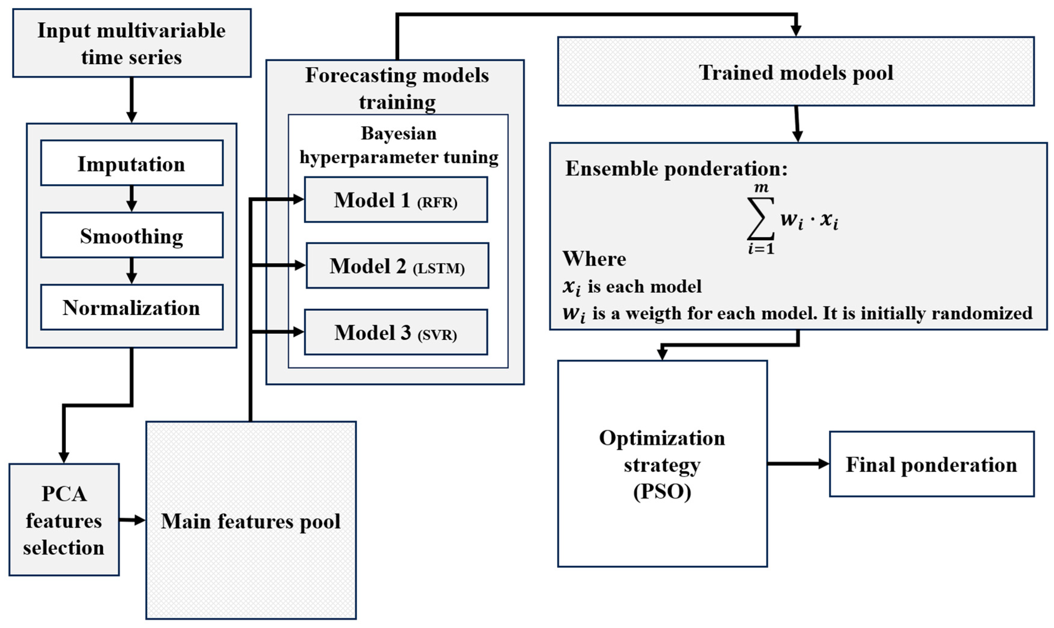
Multivariate time series forecasting represents a significant challenge due to multiple factors affecting its performance. This process requires rigorous preprocessing to ensure complete, consistent, high-quality data, eliminate outliers, and, in many cases, to solve the missing data problem. In addition, it is essential to implement feature selection strategies that reduce the problem’s dimensionality, preserving as much explained variance as possible. Subsequently, forecasting models should be trained with modern and robust machine learning techniques, selecting them for their outstanding performance on similar problems, in part of the problem; in our case, we consider it more effective to select them by their performance in the validation section of each time series. In other words, using a heuristic ensemble ensures a broad exploration of the solution space, achieving high-performance predictive models.

In this context, this paper presents an ensemble methodology for multivariate time series forecasting with feature selection, whose modular architecture is illustrated in Figure 1. Each component of the proposed model is replaceable by different techniques, which endows the methodology with flexibility and adaptability.

3.1. Time Series Preprocessing

The data used in this work come from physical weather stations, which may face conditions that generate noise or missing data in the time series. This makes a remediation process prior to model adjustment indispensable, since cured data favor a better forecast performance and reduce training times. As a first step, an imputation based on quadratic interpolation was applied. This choice responds to the data analysis, where absences are usually isolated or span less than two consecutive periods. This method uses neighboring values to estimate missingness more accurately.

To mitigate the impact of noise and outliers, two smoothing strategies were implemented. First, a moving average with a window of size two was used, which allowed smoothing time series without significantly altering their essential patterns. Subsequently, Singular Value Decomposition (SVD) was applied [12]. This technique consisted of hankelization of the series with a seasonal periodicity of 365 periods and retaining 95% of the principal components after decomposition. The hankelized series reduced noise by eliminating low-relevance components. It is important to mention that SVD is applied to each variable individually, so that information is not mixed across variables. Therefore, n strategies are applied to the model, where n is the number of variables in the system.

These strategies not only ensure data integrity for model fitting, but are also critical for capturing seasonal patterns and underlying trends in the time series. By removing noisy elements, models can focus on learning relevant information, resulting in more consistent and robust performance, especially in critical applications such as weather forecasting.

Finally, the data were normalized to the interval [1,2]. This choice was motivated by the need to avoid potential problems with forecasting methods and evaluation metrics, ensuring consistency of subsequent analysis.

3.2. Selection of Relevant Characteristics

In the field of multivariate time series, the problem of high dimensionality acquires crucial relevance due to the issues generated in adjustment and forecasting [27,28,29]. Each variable or indicator incorporated in the time series adds an additional dimension to the data set. Although it could be assumed that a greater number of variables implies an improvement in the quality of the forecast due to the increase in the amount of information available, it is essential to know that not all the information added is useful for the model. In fact, many times, these variables can be redundant, irrelevant, or introduce noise, hindering the learning process.

Increasing dimensionality also significantly increases the time and computational resources required by the models [30]. This not only lengthens the fitting process, but can negatively affect model quality due to the complexity of exploring a solution space that grows exponentially with the number of dimensions.

In this context, one of the key approaches to addressing this problem is feature selection. Proper selection involves identifying those variables that have a significant impact on the target variable, eliminating those that are highly correlated with each other or that contribute little information to the model. This process not only improves the quality of the fit, but also reduces processing time and allows a simple analysis of the relationships between the selected variables and the target.

For this work, PCA is implemented as the principal feature selection strategy, a mathematical technique that transforms the original data set into a new system defined by principal components [28]. These components are calculated from the eigenvalues and eigenvectors of the covariance matrix of the data set, where each eigenvector defines a direction in the space of the variables, and its corresponding eigenvalue represents the variance explained in that direction.

The central idea of PCA is to rearrange the dimensions of the system so that the first components capture the largest proportion of the variability present in the data. In this work, a variance explained threshold of 92% is used, which means that only those principal components whose cumulative variance exceeds this percentage are selected. This approach allows for a significant reduction in dimensionality without losing relevant information for forecasting.

Although PCA generates new variables (components) that are linear combinations of the original variables, the components are used in terms of the initial variables. In this paper, the PCA process is not completed, and it is stopped when it reaches the phase of weighting the variables with the highest explained variance, returning the necessary variables until the threshold is reached.

This facilitates a subsequent analysis of how each variable contributes to the forecast, which is essential for evaluating its impact on the target variable.

The implemented strategy not only optimizes computational efficiency, but also provides a more manageable and relevant feature set, allowing forecasting models to be fitted more accurately and quickly.

3.3. Forecasting Models

The strategies of tuning hyperparameters are performed in order to fit the data. Each strategy does this differently and performs differently in both quality and fitting time. Although there is no universally superior strategy, the strategies selected for this work stand out for their high accuracy, robustness, and reliability. These strategies have also been successfully applied to problems relating to the forecast of atmospheric variables and to issues related to climate change.

3.3.1. Long Short-Term Memory

Neural networks are a powerful approach for generalizing information and extracting complex patterns from a data set [31,32]. These networks stand out for responding accurately, even to entirely unknown data. However, their performance in time series forecasting has shown limitations because they tend to process data individually and do not explicitly consider the temporal dependencies inherent in this type of information.

To address the last limitation, LSTM offers an innovative solution [33]. These networks incorporate a structure based on specialized cells to maintain relevant information over time and discard information that is useless for future learning. This ability “to remember” and “to forget” in a controlled manner is crucial for modeling temporal dependencies in time series data, facilitating complex learning of dynamic patterns.

In this work, an LSTM neural network architecture specifically designed to address the challenges of forecasting climate change related variables has been implemented [20]. This architecture consists of LSTM cells organized in stacked layers, which allows the efficient capture of complex multivariate patterns and improves the representation of temporal dependencies in the data.

Once the LSTM cells process the information, a fully connected network (or standard dense layer) is responsible for generalizing the learned representation and providing the final model output. This combination of structures ensures an effective integration between the capture of temporal dependencies and the generalization of the learned patterns.

Table 1. LSTM configuration.

Hyperparameters *	Value
LSTM Cells	64
LSTM Layers	5
Dropout per layer	0.5
MLP layers	5
Loss function	Mean Squared Error
Early stopping patience	80
Epoch	2000

* Configuration of the LSTM model, including key hyperparameters such as the number of layers, dropout rate, and training epochs used in this study.

details the hyperparameters used in the LSTM network configuration employed in this work. These hyperparameters include the number of LSTM layers, the number of units in each layer, the learning rate, and the regularization of values applied, among others.

3.3.2. Random Forest Regression

This regression method is called RFR (that stands up Random Forest Regression). RFR belongs to the Decision Trees popular models in machine learning. RFR is widely applied in forecasting because it divides complex data into simpler subgroups [34,35,36]. RFR attractive features include a small number of tunable parameters, automatic calculation of generalization errors and handling of missing data, different types of data, and general resistance to overfitting [37]. RFR combines multiple decision trees to form a robust model using the bagging approach, where each tree is trained with random subsamples of the original data. In our case, the data consists of a time series, which allows us to identify both specific patterns and broader trends, as well as seasonal patterns.

Each tree generates an independent prediction, and, in the end, these predictions are combined by an operation (usually the arithmetic mean) to obtain the final result. This approach reduces variance and improves the model’s ability to capture complex nonlinear relationships. Figure 2 shows this flow, while

Table 2. Random Forest configuration.

Hyperparameter *	Value
Estimators	500
Max depth	10
Min samples split	10
Min samples leaf	15

* Hyperparameters used for the RFR model, detailing the number of estimators, maximum depth, and splitting criteria.

details the hyperparameters used, such as the number of trees, maximum depth, and splitting criteria.

In this work, we apply the methodology to the analysis of climate data, a domain where nonlinear relationships and complex temporal dynamics are common. Random Forest proves to be effective in identifying patterns in key variables such as temperature, precipitation, and greenhouse gas concentration, providing accurate and reliable predictions.

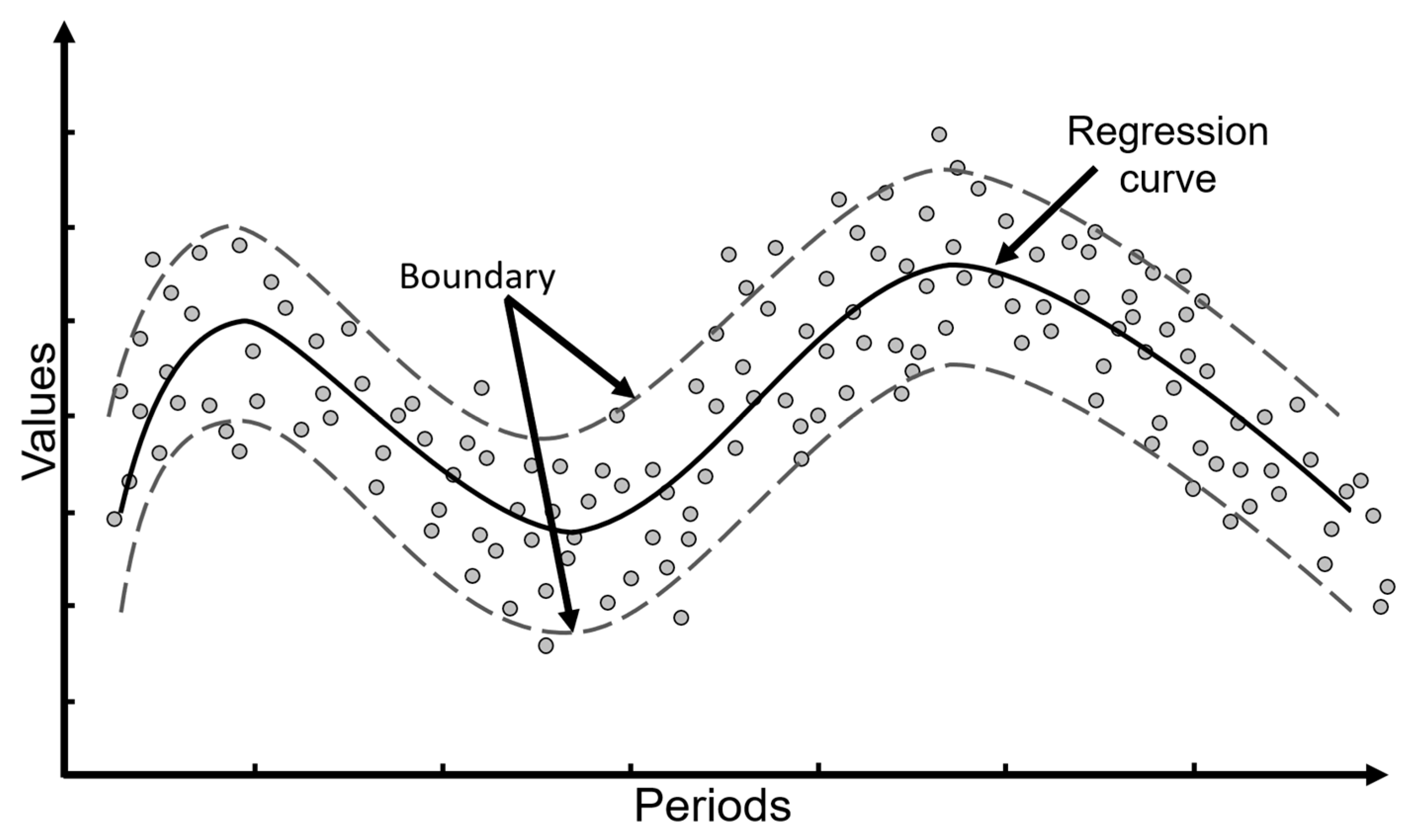
3.3.3. Support Vector Regression

Support vector regression machines are a widely used strategy for function fitting in forecasting problems [38]. This approach is based on finding a function that minimizes the prediction error while maintaining a balance between model complexity and data generalization. The main objective is to provide an efficient forecast consistent with the information used during training.

Regarding time series, SVR captures complex patterns in the data using kernel functions, which allow modeling nonlinear relationships between variables. This method is especially useful in highly nonlinear problems, and represents typical behavior of atmospheric data [39]. Figure 3 shows a graphical representation of the function fitting process using SVR. The circles in the input and output of the boundary region represent events of a general process. Moreover, the width of this boundary delimited by broken lines represents the confidence interval, delimited by the parameter ϵ or controlled margin, allowing to focus on predicting relevant patterns. The hyperparameters listed in

Table 3. SVR configuration.

Hyperparameter	Value
Kernel	RBF
C	1.0
Epsilon	0.1
Gamma	Scale

follow the standard formulation commonly adopted in the literature for SVR models [38,39]. They are the penalty parameter C, the epsilon parameter ε, and the kernel coefficient γ. The C parameter controls the trade-off between the model complexity and the degree to which deviations greater than ε are penalized. The epsilon ε defines a margin of tolerance where no penalty is given to errors, effectively shaping the SVR loss function. The configuration of the hyperparameters used, including γ, ϵ, and C, is detailed in Table 3. These hyperparameters were obtained by Bayesian experimentation [40,41].

3.4. Hyperparameter Tuning

The configuration of hyperparameters is critical to the performance of forecasting models, as it defines their ability to generalize and avoid problems such as overfitting or underfitting [40,41]. An overfitted model presents low errors in the training set, but poor performance on unknown data, while an underfitted model lacks the flexibility to capture relevant patterns.

In this work, Bayesian fitting was used to determine the optimal hyperparameters, ensuring a balance between accuracy and generalization. Bayesian fitting prioritizes well-performing configurations using an iterative probabilistic model, reducing the search space and increasing efficiency. Unlike traditional methods such as GridSearch, this approach dynamically adapts to previous results, maximizing the probability of finding optimal configurations with fewer evaluations [41].

3.5. Ensemble Strategy

Despite the tunability of forecasting models, there is no guarantee that they generalize information uniformly, since each strategy fits specific aspects of the training data. This implies that there is no universally superior model for all forecasting problems, due to the diversity and complexity of the data used for tuning [12].

Ensemble strategies address this problem by combining predictions from multiple models, taking advantage of their individual strengths and mitigating their fitting errors. In this approach, each model contributes a given weight to the final result. However, an inappropriate allocation of these weights can generate results inferior to the best individual model, making it essential to optimize this weighting.

In this work, PSO is used to determine the weights of the models in the ensemble. This heuristic technique, inspired by the behavior of natural systems, seeks efficient solutions to highly complex problems. The particle swarm begins by randomly initializing a population of candidate weight vectors, where each particle represents a possible combination of model weights. These weights are subject to the constraint that their sum equals one. During each iteration, particles evaluate their performance on the objective function, typically based on validation error, and adjust their positions in the search space based on their own best historical performance and the best performance observed in their neighborhood. This process allows the algorithm to iteratively refine the weight configuration toward an optimal or near-optimal solution [42,43].

Although PSO does not guarantee finding the globally optimal solution, its exploratory capability ensures obtaining combinations of models that at least equal the performance of the best individual model.

3.6. Error Metrics

Fitting forecast models and ensemble weighting require an accurate assessment of their performance. For this purpose, error metrics that quantify the variation between model predictions and the actual values of the time series are used. These metrics allow the models to be adjusted to minimize the prediction error, thus improving their forecasting capability. In the literature, several error metrics are found, each one focused on specific aspects of model performance [44]. However, there is no universally superior metric, as the choice depends on the type of problem, the characteristics of the data, and the purpose of the analysis. In this paper, the Mean Squared Error (MSE) is used as the main metric for model fitting. This metric is defined as $MSE={\displaystyle \frac{1}{N}}·\sum _{i=1}^N{(y_i-{\hat{y}}_i)}^2$ where $y_i$ are the real values, ${\hat{y}}_i$ are the values predicted by the model, and $N$ is the total number of observations. The MSE penalizes large errors more severely, which favors a more accurate fit by reducing significant deviations during training. However, the MSE generates results in quadratic units, which makes it difficult for users to interpret directly.

To facilitate the understanding of the results, the Mean Absolute Percentage Error (MAPE) is used as a reporting metric. This metric is defined as $MAPE={\displaystyle \frac{100}{N}}\sum _{i=1}^N\left|{\displaystyle \frac{y_i-{\hat{y}}_i}{y_i}}\right|$. The MAPE, expressed in percentage terms, provides a more intuitive and straightforward interpretation, since it indicates the average percentage relative error between predicted and actual values. This feature makes it especially useful for comparing results between different models and time series, providing a more accessible view for end users.

4. Experimental Results

This section describes the data set used during the experimental process, as well as the results obtained after the implementation of the proposed method. In addition, a comprehensive comparison is made between the performance of the ensemble method and the individual models, highlighting the advantages and limitations of each approach. All models used in this study were executed a minimum of 30 times to ensure the stability and reliability of the results. The values reported correspond to the average of these runs, allowing for a more accurate representation of the performance of each model. In addition, the runs were performed without time constraints, allowing each model to reach its best possible fit under the experimental conditions. Nevertheless, the average execution time for each strategy is also reported to provide a comparative perspective on computational efficiency.

4.1. Data Description

The information used in the experimental process of this work is based on four multivariate time series corresponding to key cities in Mexico: Monterrey, Guadalajara, Tijuana, and Tampico. The selection of these cities responds to their high susceptibility to the effects of climate change, such as extreme weather events, and their relevance as densely populated metropolises with diverse climatic environments. According to Germanwatch’s Climate Risk Index 2023, Mexico ranks 31st globally, with a high vulnerability score due to extreme weather events such as hurricanes, catastrophic storms, and prolonged droughts [3]. This situation is aggravated by its geography, with two coasts exposed to the Atlantic and Pacific Oceans, its vast territorial extension, and its complex diversity of climatic ecosystems. Furthermore, according to data from the National Institute of Statistics and Geography (INEGI), over the last 30 years, Mexico has registered an average increase of 0.85 °C in annual temperature and a notable increase in the frequency of extreme events, such as torrential rains and severe droughts [45]. In this study, the time series were formed from weather data collected daily from airport weather stations located within the selected cities. These stations, being operated under international standards, offer reliable and consistent measurements. The data set spans the period from January 2012 to December 2022, ensuring a comprehensive temporal coverage for the analysis. The variables analyzed include maximum, minimum, and average temperature; maximum average and minimum dew point; maximum and average relative humidity; maximum average and minimum wind speed; and finally, maximum, average, and minimum atmospheric pressure. The choice of these variables allows capturing a comprehensive representation of the daily weather conditions in each region. These variables are not only relevant for forecasting, but also have a direct impact on climate risk assessment. The information used in the experimental process was divided sequentially into four main blocks. The first block corresponds to the training set, which represents 55% of the time series and is used to adjust the models. The subsequent blocks are as follows: validation set 1 (15% of the data), used for hyperparameter tuning; validation set 2 (15% of the data), used to evaluate model performance under test-like conditions; and finally, the test set (15% of the data), which is used to assess the final performance of the models on data not seen during any stage of training or validation.

4.2. Experimentation

In the first instance, the proposed models were evaluated individually using the temperature target in its three representations: maximum, average, and minimum. The results obtained, presented in

Table 4. Forecasting models comparative.

Cities *	Temperature	SVR	RFR	LSTM	σ SVR	σ RFR	σ LSTM
Guadalajara	Max	2.78%	1.61%	3.27%	0	2	0.04
	Avg	2.94%	1.64%	3.73%	0	0.11	0.04
	Min	2.79%	1.58%	2.87%	0	0.01	0.11
Monterrey	Max	3.60%	2.86%	4.65%	0	0.95	0.65
	Avg	4.18%	5.71%	5.66%	0	0.74	0.07
	Min	3.08%	2.66%	6.09%	0	0.46	0.37
Tampico	Max	3.16%	3.04%	3.97%	0	0.38	3.03
	Avg	2.76%	2.89%	4.18%	0	0.05	0.30
	Min	3.16%	3.31%	3.97%	0	0.08	0.09
Tijuana	Max	5.02%	3.97%	4.07%	0	0.25	0.12
	Avg	3.56%	2.99%	4.41%	0	0.12	0.01
	Min	4.87%	3.31%	4.22%	0	0.76	0.64

* Comparison of the average error and standard deviation for the SVR, RFR, and LSTM models, evaluated on Validation Set 2 for maximum, average, and minimum temperature across cities.

, have the evaluations performed on validation set 2, which was reserved exclusively for reporting results. The forecast horizon used in this work is 15 days for each prediction.

The values indicate that the SVR and Random Forest models performed better on average in terms of percentage error than the LSTM model. However, it is important to clarify that the SVR model is deterministic under the configuration used in this study. That is, given a fixed set of hyperparameters and training data, it produces identical results across executions, resulting in a standard deviation of zero. In contrast, the Random Forest and LSTM models include stochastic components in their training processes, which leads to variability in their outputs across runs. Among these stochastic models, LSTM exhibited the lowest standard deviation, reflecting greater stability and consistency in its predictions relative to Random Forest. However, Table 4 shows two clear outliers in the standard deviation values: Guadalajara (Max, RFR: σ = 2.00) and Tampico (Max, LSTM: σ = 3.03). These cases suggest a higher variability in the model’s predictions when trained multiple times. This behavior can be explained by the randomness present in the training processes and the complexity of the data in those particular cities. Not all models respond the same way to a given data set, and a higher deviation does not necessarily mean poor performance. It may reflect that the model is more sensitive to certain features or to noise in the data. Although the average error values are relatively stable, the presence of these outliers indicates that some models may be overfitting or underfitting in specific scenarios.

Subsequently, the models were ensembled to generate a common forecast using a particle swarm algorithm, fitted with training and validation sets 1.

Table 5. Ensemble results in validation 2 set.

Cities *	Temperature	Ensemble
Guadalajara	Max	1.61%
	Avg	1.60%
	Min	1.58%
Monterrey	Max	2.59%
	Avg	3.04%
	Min	2.52%
Tampico	Max	2.62%
	Avg	2.39%
	Min	2.53%
Tijuana	Max	3.28%
	Avg	2.87%
	Min	3.10%

* Performance of the ensemble model on Validation Set 2, showing average percentage error for maximum, average, and minimum temperature predictions across cities.

presents the results of this ensemble evaluated on validation set 2, completely invisible during the fitting of both the individual models and the ensemble. The results show that the ensemble method not only improves the average performance but, in all cases, achieves results at least as good as the best individual model, with consistent improvements. This is due to the exploratory nature of the swarm algorithm, which evaluates solutions in the search space by collaboratively combining the strengths of the individual models. Once the PSO algorithm determined the optimal weight configuration based on training and validation set 1, this fixed combination was subsequently applied to the test set without further adjustments. This ensures that the evaluation on the test data remained unbiased and reflects the true generalization capacity of the ensemble model. Figure 4 graphically illustrates an example of the forecasting behavior, evidencing an excellent fit to the original curve.

Table 6. Comparative results of the ensemble with the best of the individual methods.

Cities *	Temperature	Best Model	Best Model MAPE	Ensemble MAPE	Improvement
Guadalajara	Max	RFR	1.61%	1.61%	0%
	Avg	RFR	1.64%	1.60%	2.43%
	Min	RFR	1.58%	1.58%	0%
Monterrey	Max	RFR	2.86%	2.59%	9.44%
	Avg	SVR	4.18%	3.04%	27.27%
	Min	RFR	2.66%	2.52%	5.26%
Tampico	Max	RFR	3.04%	2.62%	13.81%
	Avg	SVR	2.76%	2.39%	13.26%
	Min	SVR	3.16%	2.53%	19.93%
Tijuana	Max	RFR	3.97%	3.28%	17.38%
	Avg	RFR	2.99%	2.87%	4.01%
	Min	RFR	3.31%	3.10%	6.34%

* Comparison showing the percentage improvement between the results of the ensemble method versus the best of the individual forecasting methods obtained in the data set of each cited city.

compares the results of the best model versus those of the ensemble. It is relevant to note that, in any case, the ensemble method has a forecasting performance at least as good as the best single method.

In order to quantify the improvement in forecast accuracy using the ensemble strategy, for each data set, we present in Table 6 the percentage improvement obtained from the single best method versus the ensemble. The results show that, in most cases, the ensemble outperformed the best base model, achieving improvements of up to 27.27% in MAPE, as observed in the average temperature series for Monterrey. On average, the ensemble reduced the MAPE by 9.13% compared to the best individual model, demonstrating greater generalization capacity and robustness when dealing with multivariate climate data variability.

To evaluate the stability of the ensemble model, data from the test set were invisible during the fitting processes.

Table 7. Results in test set.

Cities *	Temperature	Ensemble
Guadalajara	Max	2.04%
	Avg	3.92%
	Min	1.93%
Monterrey	Max	5.57%
	Avg	4.32%
	Min	3.37%
Tampico	Max	2.44%
	Avg	4.55%
	Min	4.12%
Tijuana	Max	4.24%
	Avg	3.47%
	Min	5.31%

* Evaluation of the ensemble model’s performance on the test set, including average percentage error for maximum, average, and minimum temperature predictions across cities.

reports the average results in this ensemble, which represents the tail of the time series and may include new patterns or abrupt changes. Despite these challenges, the ensemble demonstrated a remarkable generalization capability, as graphically observed in Figure 5.

Regarding the computational efficiency, although the primary objective of this study was to assess the predictive performance and generalization capabilities of the ensemble model, we also report the average training times of the individual components. The SVR model required approximately 3 s per series, while RFR averaged 6.2 min, and LSTM models executed with GPU acceleration took about 8.4 min. The ensemble optimization using PSO required an average of 1.2 min per configuration. All experiments were conducted on a workstation equipped with a Ryzen 7 5700X processor, 32 GB of RAM, and an NVIDIA GeForce RTX 4060 OC, leveraging multithreading for traditional models and GPU computing for neural networks.

The proposed method stands out for its ability to integrate multiple models, improving overall performance, robustness, and generalization in multivariate time series. This approach also highlights the relevance of the selected variables by prioritizing those that contribute significantly to the final model. However, some limitations were identified, such as the dependence on the quality and completeness of the data, as well as the need to evaluate its scalability in larger data sets. In future work, this methodology can be extended to other regions and variables, as well as to explore improvements in the ensemble algorithm.

5. Conclusions

This paper presents an innovative methodology based on an ensemble approach for multivariate time series forecasting applied to climate change. The methodology combines multiple machine learning techniques with a heuristic particle swarm algorithm to select relevant features and optimize the forecasting process. The results obtained demonstrate that the ensemble approach consistently outperforms the individual models. In all cases evaluated, the ensemble strategy produced results equal to or better than the best individual model and, on average, achieved significant improvements. This situation reflects the algorithm’s ability to leverage the strengths of each model and explore optimal solutions in the search space. A highlight of the approach is its ability to generalize information. The methodology was evaluated on several test sets with distinct data patterns in each data set, with common features with observations related to climate change. Despite these difficulties, the ensemble model maintained robust performance, adapting to the inherent variability of the data and demonstrating its utility in complex stages. The inclusion of a feature selection process is also fundamental to the effectiveness of the model. This process not only reduces the dimensionality of the problem, but also retains most of the variance explained, improving the interpretability and efficiency of the model. This selection allows the model to work exclusively with the most significant variables contributing to optimal prediction performance.

As for the individual models, although SVR and Random Forest show a better average performance, the LSTM model stands out for its stability, evidenced by a lower standard deviation. This analysis confirms that the integration of complementary models within the ensemble is an effective strategy to improve both the accuracy and consistency of results. We proposed to refine the ensemble approach by incorporating Machine Learning and heuristic optimization techniques, as well as a new general architecture. In addition, the application of this methodology to other atmospheric variables and regions will be explored, deepening the understanding of climate change and its effects. With these improvements, the proposed approach has the potential to consolidate as a robust and efficient tool for global climate forecasting.

References

- Abbass, K.; Qasim, M.Z.; Song, H.; Murshed, M.; Mahmood, H.; Younis, I. A Review of the Global Climate Change Impacts, Adaptation, and Sustainable Mitigation Measures. Environ. Sci. Pollut. Res. 2022, 29, 42539–42559. [Google Scholar] [CrossRef]
- Al-Ghussain, L. Global Warming: Review on Driving Forces and Mitigation. Environ. Prog. Sustain. Energy 2019, 38, 13–21. [Google Scholar] [CrossRef]
- Jan, B.; Thea, U.; Leonardo, N.; Christoph, B. The Climate Change Performance Index 2023: Results. 2022. Available online: https://www.germanwatch.org/en/87632 (accessed on 23 January 2025).
- CMNUCC. COP 21. Available online: https://unfccc-int.translate.goog/event/cop-21?_x_tr_sl=en&_x_tr_tl=es&_x_tr_hl=es&_x_tr_pto=tc (accessed on 23 January 2025).
- Lal, R. Beyond COP 21: Potential and Challenges of the “4 per Thousand” Initiative. J. Soil Water Conserv. 2016, 71, 20A–25A. [Google Scholar] [CrossRef]
- Rodríguez-Aguilar, O.; López-Collado, J.; Soto-Estrada, A.; Vargas-Mendoza, M.d.l.C.; García-Avila, C.d.J. Future Spatial Distribution of Diaphorina citri in Mexico under Climate Change Models. Ecol. Complex. 2023, 53, 101041. [Google Scholar] [CrossRef]
- Fildes, R.; Kourentzes, N. Validation and Forecasting Accuracy in Models of Climate Change. Int. J. Forecast. 2011, 27, 968–995. [Google Scholar] [CrossRef]
- Hargreaves, J.C.; Annan, J.D. On the Importance of Paleoclimate Modelling for Improving Predictions of Future Climate Change. Clim. Past 2009, 5, 803–814. [Google Scholar] [CrossRef]
- Yerlikaya, B.A.; Ömezli, S.; Aydoğan, N. Climate Change Forecasting and Modeling for the Year of 2050. In Environment, Climate, Plant and Vegetation Growth; Fahad, S., Hasanuzzaman, M., Alam, M., Ullah, H., Saeed, M., Ali Khan, I., Adnan, M., Eds.; Springer International Publishing: Cham, Switzerland, 2020; pp. 109–122. ISBN 978-3-030-49731-6. [Google Scholar]
- Wolpert, D.H.; Macready, W.G. No Free Lunch Theorems for Optimization. IEEE Trans. Evol. Comput. 1997, 1, 67–82. [Google Scholar] [CrossRef]
- Frausto-Solis, J.; Rodriguez-Moya, L.; González-Barbosa, J.; Castilla-Valdez, G.; Ponce-Flores, M. FCTA: A Forecasting Combined Methodology with a Threshold Accepting Approach. Math. Probl. Eng. 2022, 2022, e6206037. [Google Scholar] [CrossRef]
- Estrada-Patiño, E.; Castilla-Valdez, G.; Frausto-Solis, J.; González-Barbosa, J.; Sánchez-Hernández, J.P. A Novel Approach for Temperature Forecasting in Climate Change Using Ensemble Decomposition of Time Series. Int. J. Comput. Intell. Syst. 2024, 17, 253. [Google Scholar] [CrossRef]
- Dimri, T.; Ahmad, S.; Sharif, M. Time Series Analysis of Climate Variables Using Seasonal ARIMA Approach. J. Earth Syst. Sci. 2020, 129, 149. [Google Scholar] [CrossRef]
- Zia, S. Climate Change Forecasting Using Machine Learning SARIMA Model. iRASD J. Comput. Sci. Inf. Technol. 2021, 2, 1–12. [Google Scholar] [CrossRef]
- Ray, S.; Das, S.S.; Mishra, P.; Al Khatib, A.M.G. Time Series SARIMA Modelling and Forecasting of Monthly Rainfall and Temperature in the South Asian Countries. Earth Syst. Environ. 2021, 5, 531–546. [Google Scholar] [CrossRef]
- Dabral, P.P.; Murry, M.Z. Modelling and Forecasting of Rainfall Time Series Using SARIMA. Environ. Process. 2017, 4, 399–419. [Google Scholar] [CrossRef]
- Szostek, K.; Mazur, D.; Drałus, G.; Kusznier, J. Analysis of the Effectiveness of ARIMA, SARIMA, and SVR Models in Time Series Forecasting: A Case Study of Wind Farm Energy Production. EBSCOhost. Available online: https://openurl.ebsco.com/contentitem/doi:10.3390%2Fen17194803?sid=ebsco:plink:crawler&id=ebsco:doi:10.3390%2Fen17194803 (accessed on 23 January 2025).
- Hamidi, M.; Roshani, A. Investigation of Climate Change Effects on Iraq Dust Activity Using LSTM. Atmos. Pollut. Res. 2023, 14, 101874. [Google Scholar] [CrossRef]
- Ian, V.-K.; Tang, S.-K.; Pau, G. Assessing the Risk of Extreme Storm Surges from Tropical Cyclones under Climate Change Using Bidirectional Attention-Based LSTM for Improved Prediction. Atmosphere 2023, 14, 1749. [Google Scholar] [CrossRef]
- Gong, Y.; Zhang, Y.; Wang, F.; Lee, C.-H. Deep Learning for Weather Forecasting: A CNN-LSTM Hybrid Model for Predicting Historical Temperature Data. arXiv 2024, arXiv:2410.14963. [Google Scholar]
- Bansal, N.; Defo, M.; Lacasse, M.A. Application of Support Vector Regression to the Prediction of the Long-Term Impacts of Climate Change on the Moisture Performance of Wood Frame and Massive Timber Walls. Buildings 2021, 11, 188. [Google Scholar] [CrossRef]
- Jayanthi, S.L.S.V.; Keesara, V.R.; Sridhar, V. Prediction of Future Lake Water Availability Using SWAT and Support Vector Regression (SVR). Sustainability 2022, 14, 6974. [Google Scholar] [CrossRef]
- Kumar, S. A Novel Hybrid Machine Learning Model for Prediction of CO2 Using Socio-Economic and Energy Attributes for Climate Change Monitoring and Mitigation Policies. Ecol. Inform. 2023, 77, 102253. [Google Scholar] [CrossRef]
- Holsman, K.K.; Aydin, K. Comparative Methods for Evaluating Climate Change Impacts on the Foraging Ecology of Alaskan Groundfish. Mar. Ecol. Prog. Ser. 2015, 521, 217–235. [Google Scholar] [CrossRef]
- Zhang, C.; Ma, Y. Ensemble Machine Learning: Methods and Applications; Springer: Cham, Switzerland, 2012. [Google Scholar]
- Estrada-Patiño, E.; Castilla-Valdez, G.; Frausto-Solis, J.; Gonzalez-Barbosa, J.J.; Sánchez-Hernández, J.P. HELI: An Ensemble Forecasting Approach for Temperature Prediction in the Context of Climate Change. Comput. Y Sist. 2024, 28, 1537–1555. [Google Scholar] [CrossRef]
- Lu, Y.; Cohen, I.; Zhou, X.S.; Tian, Q. Feature Selection Using Principal Feature Analysis. In Proceedings of the 15th ACM International Conference on Multimedia, Augsburg, Germany, 24–29 September 2007; ACM: New York, NY, USA, 2007; pp. 301–304. [Google Scholar]
- Malhi, A.; Gao, R.X. PCA-Based Feature Selection Scheme for Machine Defect Classification. IEEE Trans. Instrum. Meas. 2004, 53, 1517–1525. [Google Scholar] [CrossRef]
- Song, F.; Guo, Z.; Mei, D. Feature Selection Using Principal Component Analysis. In Proceedings of the 2010 International Conference on System Science, Engineering Design and Manufacturing Informatization, Yichang, China, 12–14 November 2010; Volume 1, pp. 27–30. [Google Scholar]
- Johnstone, I.M.; Titterington, D.M. Statistical Challenges of High-Dimensional Data. Phil. Trans. R. Soc. Math. Phys. Eng. Sci. 2009, 367, 4237–4253. [Google Scholar] [CrossRef]
- Gers, F.A.; Schmidhuber, J.; Cummins, F. Learning to Forget: Continual Prediction with LSTM. Neural Comput. 2000, 12, 2451–2471. [Google Scholar] [CrossRef] [PubMed]
- Agga, A.; Abbou, A.; Labbadi, M.; Houm, Y.E.; Ou Ali, I.H. CNN-LSTM: An Efficient Hybrid Deep Learning Architecture for Predicting Short-Term Photovoltaic Power Production. Electr. Power Syst. Res. 2022, 208, 107908. [Google Scholar] [CrossRef]
- Frausto-Solís, J.; Galicia-González, J.C.d.J.; González-Barbosa, J.J.; Castilla-Valdez, G.; Sánchez-Hernández, J.P. SSA-Deep Learning Forecasting Methodology with SMA and KF Filters and Residual Analysis. Math. Comput. Appl. 2024, 29, 19. [Google Scholar] [CrossRef]
- Ali, J.; Khan, R.; Ahmad, N.; Maqsood, I. Random Forests and Decision Trees. Int. J. Comput. Sci. Issues 2012, 9, 272. [Google Scholar]
- Breiman, L. Random Forests. Mach. Learn. 2001, 45, 5–32. [Google Scholar] [CrossRef]
- Altman, N.; Krzywinski, M. Ensemble Methods: Bagging and Random Forests. Nat. Methods 2017, 14, 933–935. [Google Scholar] [CrossRef]
- Auret, L.; Aldrich, C. Interpretation of Nonlinear Relationships Between Process Variables by Use of Random Forests. Miner. Eng. 2012, 35, 27–42. [Google Scholar] [CrossRef]
- Balabin, R.M.; Lomakina, E.I. Support Vector Machine Regression (SVR/LS-SVM)—An Alternative to Neural Networks (ANN) for Analytical Chemistry? Comparison of Nonlinear Methods on near Infrared (NIR) Spectroscopy Data. Analyst 2011, 136, 1703–1712. [Google Scholar] [CrossRef]
- Izonin, I.; Tkachenko, R.; Shakhovska, N.; Lotoshynska, N. The Additive Input-Doubling Method Based on the SVR with Nonlinear Kernels: Small Data Approach. Symmetry 2021, 13, 612. [Google Scholar] [CrossRef]
- Victoria, A.H.; Maragatham, G. Automatic Tuning of Hyperparameters Using Bayesian Optimization. Evol. Syst. 2021, 12, 217–223. [Google Scholar] [CrossRef]
- Wu, J.; Chen, X.-Y.; Zhang, H.; Xiong, L.-D.; Lei, H.; Deng, S.-H. Hyperparameter Optimization for Machine Learning Models Based on Bayesian Optimization. J. Electron. Sci. Technol. 2019, 17, 26–40. [Google Scholar]
- Kennedy, J.; Eberhart, R. Particle Swarm Optimization. In Proceedings of the ICNN’95-International Conference on Neural Networks, Perth, Australia, 27 November–1 December 1995; Volume 4, pp. 1942–1948. [Google Scholar]
- Wang, D.; Tan, D.; Liu, L. Particle Swarm Optimization Algorithm: An Overview. Soft Comput. 2018, 22, 387–408. [Google Scholar] [CrossRef]
- Hyndman, R.; Koehler, A.B.; Ord, J.K.; Snyder, R.D. Forecasting with Exponential Smoothing: The State Space Approach; Springer Science & Business Media: Berlin, Germany, 2008; ISBN 978-3-540-71918-2. [Google Scholar]
- Geografía y Medio Ambiente. Climatológicos. Available online: https://www.inegi.org.mx/temas/climatologia/ (accessed on 23 January 2025).